


1. Introduction
Channels whose shape and evolution are determined by the interaction with the flow are common in nature – examples include alluvial rivers (Glover & Florey Reference Glover and Florey1951; Parker Reference Parker1978a), ice streams (Echelmeyer et al. Reference Echelmeyer, Harrison, Larsen and Mitchell1994) or blood vessels (Rodbard Reference Rodbard1975). In alluvial rivers, for example, the sediment is transported by the slight deviations from the threshold stress needed to dislodge a grain from the bed (Parker Reference Parker1978b). The fact that these deviations are small makes the river's shape sensitive to the detailed distribution of the stress across the stream. The problem of estimating stress across a channel is therefore, both important, due to its implications for landscape evolution (Métivier & Barrier Reference Métivier and Barrier2012), and difficult, since the estimate needs to be accurate (Popović et al. Reference Popović, Devauchelle, Abramian and Lajeunesse2021).
When the flow in the channel is steady, the friction on the bottom consumes all of the momentum injected by gravity into the overlying fluid. In the idealised case of a flow over a flat, inclined plane with a slope  $S$, this basic balance requires that the stress,
  $\tau\!$, on the channel's bottom be proportional to the flow depth,
  $D$. Even when the channel is not completely flat in the cross-stream direction, this proportionality still approximately holds at each point,
  $y$, across the stream, provided that the depth,
  $D(y)$, varies slowly enough with
  $y$, i.e.
 \begin{equation} \tau(y) \approx \rho g S D(y) , \end{equation}
where  $\rho$ is the fluid density and
  $g$ is the acceleration due to gravity. This is a simple form of the ‘shallow-water’ approximation.
The shallow-water theory of (1.1) ignores any transfer of momentum between adjacent fluid columns. Despite its simplicity, it was successfully used to describe the shape of straight, laboratory rivers with a laminar flow that carry no sediment (Seizilles et al. Reference Seizilles, Devauchelle, Lajeunesse and Métivier2013). Building on this work, Abramian, Devauchelle & Lajeunesse (Reference Abramian, Devauchelle and Lajeunesse2020) performed similar experiments with laminar rivers that carried sediment, while Popović et al. (Reference Popović, Devauchelle, Abramian and Lajeunesse2021) developed a theory to describe the shape of such rivers. The theory of Popović et al. (Reference Popović, Devauchelle, Abramian and Lajeunesse2021) made clear that the shallow-water approximation was not sufficient to describe rivers that carry sediment – the properties of such rivers were critically affected by the transfer of momentum across the stream.
Here, we are mainly motivated by extending the above theory from laminar rivers to natural ones. As a first step towards that end, we investigate the simplest case relevant to this problem – a turbulent flow driven by gravity in a straight, open channel with a fixed cross-section. We aim to find an approximation for the stress,  $\tau (y)$, across the bed of such a channel that goes beyond the shallow-water theory, and captures the first-order effects of turbulent momentum transfer. In such a flow, approximations based only on first principles are not available – the flow is unsteady and complicated, as turbulent eddies mix the fluid, and secondary flows organise into recirculation cells (Tominaga et al. Reference Tominaga, Nezu, Ezaki and Nakagawa1989; Blanckaert, Duarte & Schleiss Reference Blanckaert, Duarte and Schleiss2010; Chauvet Reference Chauvet2014).
Many models that deal with the turbulent transfer of momentum were developed in the context of flood management (Bousmar & Zech Reference Bousmar and Zech1999; Martin-Vide & Moreta Reference Martin-Vide and Moreta2008; Proust et al. Reference Proust, Bousmar, Riviere, Paquier and Zech2009; Kaddi et al. Reference Kaddi, Cierco, Faure and Proust2022). These models typically split the channel into several regions (such as the deep main channel and the shallow floodplain) and parameterise the interaction between them. However, this splitting does not yield a continuous distribution of the stress,  $\tau (y)$, across the channel. Possibly the simplest model that does this was presented in Wark, Samuels & Ervine (Reference Wark, Samuels and Ervine1990), and developed earlier in Samuels (Reference Samuels1985) starting from the Navier–Stokes equations. There, the shallow-water approximation of (1.1) was supplemented with an empirical term for the turbulent diffusion of momentum, allowing one to calculate the profiles of stress and velocity across the stream,
  $\tau (y)$ and
  $U(y)$, by solving an ordinary differential equation (ODE). Similar models, such as that of Shiono & Knight (Reference Shiono and Knight1991), were developed along the same lines to include additional effects, such as those due to secondary flows.
In this paper we develop a model along similar lines as Wark et al. (Reference Wark, Samuels and Ervine1990). Our goal is to examine this model in detail, and show that it can be used within a broader theory of river self-organisation. To make clear the assumptions that go into the model, we start from a depth-integrated momentum balance (§ 2), and derive the model from dimensional analysis and symmetry arguments under several broad assumptions about the nature of the turbulent flow, without invoking the Navier–Stokes equations (§ 3). This model corrects the shallow-water theory to first order in a channel with slowly varying bed topography. The distribution of the stress across the stream,  $\tau (y)$, in this model is a solution to a second-order linear ODE with two dimensionless parameters (§ 4) – the diffusion parameter for the stress,
  $\chi$, which controls the magnitude of the cross-stream flux of momentum and the local-shape parameter,
  $\alpha$, which controls the effect of the local variations of the channel's shape on the flux. By assuming that the momentum is carried across the stream by the largest eddies and recirculation cells, whose size is comparable to the flow depth and that move at about the frictional velocity, we estimate the orders of magnitude of
  $\chi$ and
  $\alpha$. This model predicts a smooth stress distribution across the stream on scales comparable to the flow depth – when there are strong recirculation cells in the flow, the model predicts a reasonable average stress over several such cells, while significant deviations can remain on the scale of an individual cell.
We then proceed to explore this model in the full range of its parameters. Interestingly, we find that fixing the parameters at  $\chi = 1/3$ and
  $\alpha = 1$ approximately describes the stress in a laminar flow, a result that connects natural rivers with small-scale laboratory experiments (§ 4.1). When the flow is turbulent, these parameters can, in principle, take any value, so we investigate how they affect the stress distribution in channels of various shapes, and demonstrate the qualitative effects of the cross-stream transfer of momentum, some of which may have important implications for river formation (§ 5). Finally, we suggest values of the parameters
  $\chi$ and
  $\alpha$ for practical use. We show that our model with these parameters provides a reasonable agreement with experiments and field data (§ 6). For this reason, and because it is simple and interpretable, it can serve as a basis for a minimal model of self-formed alluvial rivers.
2. Momentum balance
We consider the following problem: a turbulent fluid is driven by gravity down a straight, open channel with a fixed depth profile,  $D(y)$, and a downstream slope,
  $S$ (figure 1a). Here,
  $y$ is the cross-stream coordinate,
  $x$ is the downstream coordinate and
  $z$ is the coordinate normal to the free surface of the fluid, which we assume to be flat. The slope,
  $S$, is defined as the sine of the angle the channel makes with the horizontal, and is typically small in rivers (
 $10^{-5}$ to
  $10^{-2}$, Métivier et al. Reference Métivier2016). We assume that all properties of the flow are uniform on average in the
  $x$ direction so that we only need to consider the flow in the
  $(y,z)$ plane. We attempt to find the time-averaged stress,
  $\tau (y)$, the fluid exerts at each point across the channel bottom, as well as the lateral profile of the vertically averaged downstream velocity,
  $U(y)$. For convenience, we summarise a list of symbols we use throughout the paper in table 1.

Figure 1. (a) Turbulent flow in a straight, open channel. The depth profile,  $D(y)$, is constant along the downstream direction,
  $x$, and varies along the cross-stream direction,
  $y$. At each point across the profile, the normal to the bed makes an angle
  $\phi$ with the
  $z$ axis. The channel makes a constant downstream slope,
  $S$, with the horizontal. The upper surface is flat and open. (b) Momentum balance in a portion of the channel between coordinates
  $y_1$ and
  $y_2$. The length of the channel section along the bed is
  $\ell$. Momentum is injected into the section by gravity, and is lost to friction at the bottom. It is transferred across the boundaries at
  $y_1$ and
  $y_2$ by the flow.
Table 1. Symbols used throughout the paper.

We begin by examining the balance of streamwise momentum within a portion of the channel between two vertical slices at locations  $y_1$ and
  $y_2$ (figure 1b). Gravity injects momentum into this portion at a rate
  $\int _{y_1}^{y_2} \rho g S D \,\mathrm {d} y$, where
  $\rho$ is the fluid density and
  $g$ is the acceleration due to gravity. The turbulent flow moves momentum in and out of the portion through its vertical sides. In steady state, all the momentum that enters the section is lost to friction along the bed, which occurs at a rate
  $\int _\ell \tau \, \mathrm {d}\ell$, where the integral is performed over the arc,
  $\ell$, of the bed between
  $y_1$ and
  $y_2$. Altogether, the balance of streamwise momentum for this section of the fluid reads
 \begin{equation} \int_{y_1}^{y_2} \rho g S D \,\mathrm{d} y + F(y_1) - F(y_2) = \int_\ell \tau\, \mathrm{d}\ell , \end{equation}
where  $F$ is the flux of momentum across the stream, i.e. the net momentum that crosses a vertical slice of the channel per unit time and length in the streamwise direction (the units of
  $F$ are
  $\text {kg}\ \text {s}^{-2}$). Bringing
  $y_1$ and
  $y_2$ infinitesimally close to each other, we find the differential form of this balance:
 \begin{equation} \rho g S D - \frac{\mathrm{d}F}{\mathrm{d} y} = \tau \frac{\mathrm{d}\ell}{\mathrm{d} y} . \end{equation}
The term  $\mathrm {d} \ell /\mathrm {d} y$ is a geometric factor related to the angle,
  $\phi$, between the bed's normal vector and the
  $z$ axis (
 $\mathrm {d}\ell /\mathrm {d} y = 1/\cos \phi$). Since the tangent of
  $\phi$ equals the local slope of the channel cross-section,
  $\tan \phi = \mathrm {d}D/\mathrm {d} y$, this term can also be expressed in terms of the depth as
  $\mathrm {d}\ell /\mathrm {d} y = (1+(\mathrm {d}D/\mathrm {d} y)^2)^{1/2}$. With this, we find the momentum balance equation as
 \begin{equation} \rho g S D - F' -\tau \big(1 + D'^2\big)^{1/2} = 0 , \end{equation}
where the primes stand for derivatives with respect to  $y$. This equation did not require any assumption about the flow – it is equally valid for laminar and turbulent flows.
The specifics of the flow determine how the momentum flux,  $F$, is related to other properties, such as the velocity or the shape of the channel. Ignoring the momentum flux (
 $F = 0$), and assuming that the bed is nearly flat (
 $D' \approx 0$), we recover the shallow-water approximation of (1.1):
 \begin{equation} \tau_{{sw}}(y) = \rho g S D(y) , \end{equation}
where we used the subscript ‘ ${sw}$’ to specifically denote the stress in this approximation. Our goal here is to go beyond this approximation, and estimate
  $F$ to the lowest non-trivial order, on a variable bed. We do this in the following section.
3. Flux of momentum in a turbulent flow
Due to the complicated nature of turbulent flows, it is challenging to connect the macroscopic properties of the flow, such as the flux of momentum,  $F$, to the Navier–Stokes equations that describe the basic laws of fluid motion (Pope Reference Pope2011). For this reason, here we develop a simple model for the flux,
  $F$, without explicit reference to the Navier–Stokes equations, and confirm it later in § 6 by comparison with measurements. We start by giving examples of physical mechanisms that can give rise to different fluxes (§ 3.1). Afterwards, we use dimensional analysis to mathematically derive a first-order model for the flux on a slowly varying bed under some generic assumptions about the flow (§ 3.2).
3.1. Physical picture
Much of the phenomenology of turbulent flows can be derived from the conceptual framework of ‘turbulent eddies’ that transfer energy from large to small scales through Kolmogorov's energy cascade (Richardson Reference Richardson1920; Prandtl Reference Prandtl1925; Taylor Reference Taylor1935). More recently, this physical picture was used to relate the turbulent energy spectrum to macroscopic properties of the flow, such as the vertical velocity profile and the friction coefficient (Gioia & Bombardelli Reference Gioia and Bombardelli2001; Gioia & Chakraborty Reference Gioia and Chakraborty2006; Gioia et al. Reference Gioia, Guttenberg, Goldenfeld and Chakraborty2010). If the motion of the eddies is random, they will induce a diffusion of momentum across the stream with a diffusivity,  $\mathcal {D}_e$, proportional to their velocity,
  $V$, and length scale,
  $L$ (
$L$ ( $\mathcal {D}_e \propto V L$). These eddies mix the fluid from different parts of the flow so that they can generate a flux of momentum,
  $F$, across the stream if the downstream velocity,
  $u(y,z)$, varies throughout the flow, as in figures 2 and 3. In figure 2 the bed is flat (
 $D' = 0$), the flow is uniform in the vertical (
 $\partial u / \partial z = 0$), while the depth-averaged velocity,
  $U(y)$, varies across the stream; in figure 3 the bed has a slope (
 $D' \neq 0$), the velocity,
  $u(z)$, varies along the vertical, while its depth average is uniform across the stream (
 $U' = 0$). We now consider the flux,
  $F$, in these two configurations, assuming that the variations of
  $D(y)$ and
  $U(y)$ across the stream are slow.

Figure 2. Momentum transfer by large eddies in a flow with a horizontal velocity gradient,  $U'$, but a constant vertical velocity profile. This figure shows eddies rotating in the vertical,
  $y$–
$y$– $z$, plane, but the same analysis applies to those rotating in the horizontal,
  $x$–
$x$– $y$, plane. Lighter shades of blue indicate faster flow. The largest eddy has a horizontal scale,
  $L$, comparable to the depth,
  $D$, and a velocity
  $V$ comparable to the frictional velocity,
  $U^* = C_f^{1/2}U$. The downstream flow velocity,
  $U$, varies slowly in the transverse direction from
  $U(y-L/2)$ to
  $U(y+L/2)$ across the scale of the eddy. The eddy mixes the fluid of momentum
  $\rho U(y-L/2)$ with the fluid of momentum
  $\rho U(y+L/2)$ across a vertical slice (vertical dashed line). The flux of momentum integrated along this section is proportional to
  $F \sim \rho D V (U(y-L/2) - U(y+L/2))$ (3.1).

Figure 3. Momentum transfer in a flow with a vertical velocity profile,  $u(z)$, and a topography gradient,
  $D' < 0$, but no horizontal gradient of the depth-averaged velocity,
  $U' = 0$. (a) Vertical profiles of velocity at two locations across the stream,
  $y_1$ and
  $y_2$. The profiles are arbitrarily assumed to be quadratic,
  $u(y,z) = \tfrac {3}{2} U [ 1 - z^2/D(y)^2 ]$. A horizontal velocity gradient develops from the deeper to the shallower part of the flow, inducing a corresponding flux of momentum across the stream,
  $F$. (b) Part of the channel corresponding to panel (a). Lighter shades of blue indicate faster flow.
Let us first consider the example of figure 2. In this case, eddies of size  $L$ and velocity
  $V$ carry the downstream momentum across a vertical slice of the channel located at
  $y$, mixing the fluid from
  $y + L/2$ with the fluid from
  $y - L/2$. The parcels of fluid from
  $y + L/2$, therefore, carry about
  $\rho U(y+L/2)$ of momentum and cross the vertical slice in the negative
  $y$ direction, while those from
  $y-L/2$ carry about
  $\rho U(y-L/2)$ of momentum and cross the section in the positive
  $y$ direction. The flux,
  $F$, from these eddies represents the net total amount of momentum that crosses the vertical slice of height
  $D$ per unit time, so it is about
 \begin{equation} F \sim \rho D V [U(y-L/2) - U(y+L/2)]. \end{equation}
If the downstream flow velocity,  $U$, varies slowly across the channel, we can approximate the difference in (3.1) as
  $U(y -L/2) - U(y+L/2) \approx -L U'$, so that the flux generated by these eddies is approximately
 \begin{equation} F \sim \rho D V L U' . \end{equation}
Empirically, in wide channels with a rough bottom, eddies reach a size,  $L$, comparable to the flow depth,
  $D$, since eddies much larger than this are suppressed by friction at the bottom (Bouchez et al. Reference Bouchez, Lajeunesse, Gaillardet, France-Lanord, Dutra-Maia and Maurice2010) – it matters little whether these eddies rotate in the vertical,
  $y$–
$y$– $z$, plane (as in figure 2) or in the horizontal,
  $x$–
$x$– $y$, plane. According to Kolmogorov's theory, the largest eddies in the flow also move the fastest, so that their diffusivity,
  $\mathcal {D}_e \propto LV$, is the greatest. We can, therefore, expect that these eddies are responsible for carrying most of the momentum across the stream, and for setting the mixing length (Prandtl Reference Prandtl1925). The flux of momentum induced by turbulence scales with the square of the velocity fluctuations (Batchelor Reference Batchelor1967), so that the stress, which balances the flux of momentum into the channel's bottom, should scale with the square of the eddy velocity,
  $\tau \sim \rho V^2$. Therefore, the velocity of the largest eddies should be of the order of the frictional velocity
  $U^* = \sqrt {\tau /\rho }$. On the other hand, the stress is related to the mean downstream velocity,
  $U$, through the empirical friction coefficient,
  $C_f$, as
  $\tau = \rho C_f U^2$. Thus, the velocity,
  $V$, of the largest eddies, although much smaller, is proportional to the downstream velocity,
  $V \sim C_f^{1/2} U$. Using the scalings
  $L \sim D$ and
  $V \sim C_f^{1/2} U$ in (3.2), we can write the flux,
  $F$, as
 \begin{equation} F \approx- \varLambda \rho C_f^{1/2} D^2 \big(U^2\big)' , \end{equation}
where  $\varLambda$ is a positive, dimensionless number of order one, and the minus sign ensures that the momentum is transferred from fast- to slow-flowing regions. The parameter
  $\varLambda$ controls the magnitude of the flux and we call it the dimensionless diffusion parameter.
We now consider the example of figure 3. In this case, a flux of momentum develops across the stream even though the depth-averaged velocity is uniform ( $U(y) = \text {const.}$), due to a combination of a sloping bed (
 $D' \neq 0$) and a variable vertical velocity profile (
 $\partial u / \partial z \neq 0$). A non-constant vertical profile of velocity means that some eddies will generate a flux of momentum, while the bed slope,
  $D' \neq 0$, breaks the left–right symmetry and induces a horizontal velocity gradient,
  $\partial u / \partial y$ (figure 3a). If mixing is isotropic, the momentum flux across a vertical slice is proportional to this horizontal gradient, and the total flux,
  $F$, scales as
  $F \sim \rho V \int _{-D}^0 [ \partial u / \partial y ] \,\text {d}z$, where
  $V$ is the velocity of the dominant eddies. Since the horizontal velocity gradient is, in this case, generated by the sloping bed, to first order it scales as
  $\partial u / \partial y \sim U D'$, and the flux,
  $F$, is therefore
 \begin{equation} F \sim \rho V U D D' . \end{equation}
Using  $V\sim C_f^{1/2} U$, we find an approximate expression for the flux in this configuration:
 \begin{equation} F \approx- \alpha \varLambda \rho C_f^{1/2} U^2 \big(D^2\big)' . \end{equation}
Here  $\alpha$ is another dimensionless number of order one, and we keep
  $\varLambda$ for later convenience. This flux is proportional to the depth gradient,
  $D'$, so that it appears to be induced by the bed topography. For this reason, we call
  $\alpha$ the ‘local-shape parameter.’ The minus sign in (3.5) means that when
  $\alpha$ is positive, the flux is generated from the deeper to the shallower parts of the flow. If the vertical profile of velocity,
  $u(z)$, is top heavy, meaning that the flow is faster near the free surface than at the bottom, a horizontal velocity gradient will indeed develop from deeper to shallower parts of the flow (figure 3). Therefore, positive values of
  $\alpha$ indicate a top-heavy velocity profile, while
  $\alpha$ vanishes in the ‘plug flow’ limit, i.e. when the velocity is constant along the vertical,
  $u(z) = \text {const}$.
Equations (3.3) and (3.5) for the flux,  $F$, have a similar form, only differing in the position of the cross-stream derivative – in both cases, the flux is proportional to
  $D^2$ and to
  $U^2$. The term
  $D^2$ can be interpreted as a product of the depth,
  $D$, of the vertical slice through which the transfer of momentum occurs and the length scale,
  $L$, of the dominant eddies, while the term
  $U^2$ can be interpreted as a product of the eddy velocity,
  $V$, and the downstream velocity that carries the momentum,
  $U$. In agreement with the discussion above, previous experimental studies suggest that the diffusion parameter
  $\varLambda$ is of order one. For example, Okoye (Reference Okoye1970) showed experimentally that the dimensionless eddy diffusivity,
  $\mathcal {D}_e / (2 C_f^{1/2} U D)$, analogous to our
  $\varLambda$, is of order one, varying between about
  $0.03$ and
  $1.0$. Although we also expect the local-shape parameter,
  $\alpha$, to be of order one, it likely vanishes as the flow becomes more and more turbulent, and its velocity profile starts to resemble a vertically uniform ‘plug’ flow. In Appendix A we estimate the values of
  $\varLambda$ and
  $\alpha$ in a standard model of turbulent diffusion, assuming a logarithmic vertical profile of velocity. There, we find
  $\varLambda \approx 0.03$, and
  $\alpha$ vanishing logarithmically with the Reynolds number.
In addition to unsteady eddies, turbulent flows often develop long-lived, coherent secondary currents (Znaien et al. Reference Znaien, Hallez, Moisy, Magnaudet, Hulin, Salin and Hinch2009; Shih, Hsieh & Goldenfeld Reference Shih, Hsieh and Goldenfeld2016). In channel flows with large aspect ratios, these secondary currents form an array of counter-rotating cells that have length scales comparable to the depth, and a transverse velocity of the order of the frictional velocity (Tominaga et al. Reference Tominaga, Nezu, Ezaki and Nakagawa1989; Blanckaert et al. Reference Blanckaert, Duarte and Schleiss2010; Chauvet Reference Chauvet2014). Therefore, the scalings we introduced previously should still hold for momentum transfer across these cells, even though the momentum transfer on the scale of an individual cell is not diffusive. Thus, if  $D(y)$ and
  $U(y)$ vary slowly over the scale of a single cell, we expect (3.3) and (3.5) to approximately capture the average transfer of momentum smoothed over several cells, although they cannot be accurate at the scale of a single cell.
3.2. Dimensional analysis
In the previous section we estimated the flux of momentum,  $F$, in two specific configurations of the flow based on physical reasoning. We now derive a generic, first-order expression for the flux,
  $F$, using dimensional analysis. To that end, we make the following broad assumptions about the turbulent flow.
(i) Inertial turbulent regime: Gravity,
 $g$, molecular viscosity, $\nu$, and the bed roughness, $k_s$, do not explicitly change the flux, $F$. This is certainly not exactly correct – molecular viscosity, $\nu$, and the relative roughness of the bed, $k_s/D$, both affect the friction coefficient, which can affect the momentum transfer. Nevertheless, we assume that this dependence is weak enough to remove $g$, $\nu$ and $k_s$ from the list of parameters that can affect the flux. We will later relax this assumption by allowing the model parameters to weakly depend on $g$, $\nu$ and $k_s$.
(ii) Single layer: The depth-averaged downstream velocity,
$U$, is sufficient to characterise the vertical velocity profile of the flow. In other words, we assume that the vertical velocity profile does not change its shape across the stream, so that we do not need to keep track of higher-order moments of the velocity.(iii) Locality: The flux,
$F$, is locally related to the flow speed and depth. In other words, the flux $F(y)$ is a function of the local depth-averaged velocity, $U(y)$, depth, $D(y)$, and their derivatives up to some finite order, $U'$, $D'$, $U''$, $D''$, etc. However, we assume that it does not depend on the far-away parts of the flow (such as a distant wall), nor on the integrated properties of the flow, such as the total flow discharge.(iv) Slow variation: Finally, we assume that the changes in
$D$ and $U$ occur over large scales, so that their higher-order derivatives are much smaller than the lower-order ones, and the flux can be written as an expansion in terms of these derivatives. This is likely true in a channel with a large aspect ratio. Therefore, we neglect second- and higher-order derivatives when writing a model for $F$. In this sense, our model is a first-order correction to the shallow-water theory.


Based on the above, our cross-stream flux of momentum,  $F$, can only depend on the fluid density,
  $\rho$, the local velocity,
  $U(y)$, and depth,
  $D(y)$, as well as their derivatives up to some finite order,
  $U'$,
$U'$,  $D'$,
$D'$,  $U''$,
  $D''$, etc. The most general way to construct a quantity with the units of flux (
 $\text {kg}\ \text {s}^{-2}$) from the quantities above is
 \begin{equation} F = \rho U^2 D \varPhi(D', DU'/U, \ldots) , \end{equation}
where  $\varPhi$ is an arbitrary dimensionless function of dimensionless parameters and ‘
 $\cdots$’ stands for higher-order derivatives written in dimensionless form. This equation states that the dimensionless flux,
  $F/\rho U^2 D$, can only depend on dimensionless variables, such as
  $D'$ and
  $DU'/U$ (Barenblatt Reference Barenblatt1996). Since we are looking for the lowest-order model for
  $F$, we can expand the function
  $\varPhi$ as
  $\varPhi \approx c_0 + c_1 D' + c_2 DU'/U + \cdots$, for some constants
  $c_0$,
  $c_1$ and
  $c_2$. However, since the flux is a directed quantity, it should also change sign if we mathematically flip the orientation of the
  $y$ axis,
  $F \rightarrow -F$ as
  $y\rightarrow -y$. The constant term,
  $c_0$, does not obey this symmetry, and, therefore, must vanish. To lowest order, therefore,
 \begin{equation} F \approx- \rho C_f^{1/2} \varLambda \big[D^2 (U^2)' + \alpha U^2 (D^2)'\big] , \end{equation}
where  $\varLambda$ and
  $\alpha$ are dimensionless numbers. We included the term
  $C_f^{1/2}$ in the definition of
  $\varLambda$, as in § 3.1, for convenience. Even though we assumed that the flux,
  $F$, does not depend on molecular viscosity, bed roughness or the integrated properties of the flow in order to reduce the number of parameters in the dimensional analysis, we can somewhat relax this assumption and allow the constants
  $C_f$,
  $\varLambda$ and
  $\alpha$ to weakly depend on these properties, as they likely do.
Equation (3.7) consists of two terms that correspond exactly to (3.3) and (3.5). Although the physical mechanisms we discussed in the previous section are representative of these terms, (3.7) is a generic first-order expression that does not depend on the detailed dynamics of the flow – only the values of the parameters  $C_f$,
  $\varLambda$ and
  $\alpha$ do. If eddies and recirculation cells of a size comparable with the flow depth dominate the momentum transfer, we expect
  $\varLambda$ and
  $\alpha$ to be of order one, with
  $\alpha$ vanishing in the highly turbulent, ‘plug flow’ limit (§ 3.1). On the other hand, wide recirculation cells or eddies much larger than the flow depth, cannot be included in our model since they induce a fundamentally non-local flux, violating one of our key assumptions. In Appendix A we show that a standard model of turbulent diffusion satisfies (3.7). In this sense, we may also call (3.7) a diffusive approximation.
Equation (3.7) can also be written in the compact form
 \begin{equation} F =-\rho C_f^{1/2} \varLambda D^{2(1-\alpha)} ( D^{2\alpha} U^2 )' . \end{equation}
From here, we can see that the local-shape parameter  $\alpha$ determines the part of
  $D^2$ inside the derivative. In this way, it controls the quantity that diffuses due to the flux,
  $F$ – if
  $\alpha = 0$, it is the depth-averaged velocity,
  $U$, while if
  $\alpha = 1$, it is the depth-integrated momentum,
  $DU$.
$DU$.
Wark et al. (Reference Wark, Samuels and Ervine1990) proposed a model similar to (3.7). However, they do not explicitly include the local-shape parameter,  $\alpha$, but rather mention two alternative models – one in which the velocity,
  $U$, diffuses, and another one in which it is the depth-integrated momentum
  $DU$ (‘unit flow’ in their terminology). Therefore, they consider two cases corresponding to
  $\alpha = 0$ and
  $\alpha = 1$, and state that it is unclear which one is better. Here we show that these cases are not necessarily special, so that models with non-integer values of
  $\alpha$ may also be appropriate within the same order of approximation. Besides Wark et al. (Reference Wark, Samuels and Ervine1990), we are not aware of anyone else who explicitly considered this parameter. Moreover, to our knowledge their model and its consequences have not been carefully examined.
4. Stress on the channel bottom
In the previous section we expressed the cross-stream flux of momentum,  $F$, in terms of the depth,
  $D$, and velocity,
  $U$ (3.7). In this section we show how we can use this result to find the stress,
  $\tau\!$, on the channel's bed.
As we mentioned in the previous section, the velocity in a turbulent flow is usually related to the bed stress through the friction coefficient  $C_f$ (Chézy Reference Chézy1775),
 \begin{equation} \tau = \rho C_f U^2 . \end{equation}
The friction coefficient depends on the characteristics of the flow, such as the Reynolds number and the bed roughness (Nikuradse Reference Nikuradse1933). The phenomenological equation of Colebrook (Reference Colebrook1939) summarises this dependence in circular pipes, and is often used to estimate the friction coefficient in other geometries for which direct measurements are not available. According to this approximation, the friction coefficient can be found as  $C_f = f_D/8$, where the Darcy friction factor,
  $f_{D}$, is the solution to
 \begin{equation} \frac{1}{\sqrt{f_{D}}} =-2 \log_{10}\left(\frac{k_s}{3.7 R_h} + \frac{2.51}{{Re} \sqrt{f_{D}}}\right) , \end{equation}
where  ${Re} = UD/\nu$ is the Reynolds number,
  $R_h = \mathcal {A}/\mathcal {P}$ is the hydraulic radius of the channel, equal to the ratio of the channel cross-sectional area,
  $\mathcal {A}$, to its wetted perimeter,
  $\mathcal {P}$, and
  $k_s$ is the so-called ‘Nikuradse equivalent sand roughness’, a parameter that measures the hydraulic roughness of the bed, and vanishes on a smooth bed. The typical values of the friction coefficient,
  $C_f$, for experimental flumes and large rivers range between
  $10^{-3}$ and
  $10^{-2}$ (Lajeunesse, Malverti & Charru Reference Lajeunesse, Malverti and Charru2010a).
Using (4.1) with our expression for the flux (3.7), and assuming the friction coefficient,  $C_f$, is constant across the channel, we find the flux expressed in terms of the stress:
 \begin{equation} F =- \chi \big[ D^2 \tau' + \alpha (D^2)' \tau \big] . \end{equation}
Here we introduced the diffusion parameter for the stress,  $\chi \equiv \varLambda C_f^{-1/2}$. For the typical values of
  $C_f$ we mentioned above, we expect this parameter to be about
  $\chi \sim 10$.
Combining (4.3) with the momentum balance (2.3), and assuming  $\chi$ is constant across the channel, we find a differential equation for the stress:
 \begin{equation} \chi \big( D^2 \tau' + \alpha (D^2)' \tau \big)' -\tau \big(1 + D'^2\big)^{1/2} + \rho g S D = 0. \end{equation}
For a given depth profile,  $D(y)$, and the downstream slope,
  $S$, (4.4) is a linear, second-order, ODE for
  $\tau (y)$. We can further simplify it by rescaling the lengths and stress as
 \begin{equation} \tilde{y} = \frac{y}{R_h}, \quad \tilde{D} = \frac{D}{R_h}, \quad \tilde{\tau} = \frac{\tau}{\rho g S R_h} . \end{equation}
The equation for the stress in terms of these dimensionless variables becomes
 \begin{equation} \chi \big( \tilde{D}^2 \tilde{\tau}' + \alpha (\tilde{D}^2)' \tilde{\tau}\big)' -\tilde{\tau} \big(1 + \tilde{D}'^2\big)^{1/2} + \tilde{D} = 0 , \end{equation}
where the primes now stand for derivatives with respect to  $\tilde {y}$. This rescaling ensures that the dimensionless stress averages to one over the entire channel (
 $\langle \tilde {\tau } \rangle = 1$), a result that readily follows from the integrated momentum balance of (2.1).
Equation (4.6) contains two dimensionless parameters – the diffusion parameter for the stress,  $\chi$, and the local-shape parameter,
  $\alpha$. Converting from dimensionless stress,
  $\tilde {\tau }(\tilde {y})$, to the physical one,
  $\tau (y)$, simply requires multiplying by a factor of
  $\rho g S R_h$. Therefore, for a given channel geometry, the physical stress,
  $\tau\!$, depends only on the diffusion parameter,
  $\chi$, and the local-shape parameter,
  $\alpha$, which are set by the details of the flow. Thus, the stress does not depend on the diffusion parameter,
  $\varLambda$, and the friction coefficient,
  $C_f$, independently, but only on their combination,
  $\chi = \varLambda C_f^{-1/2}$.
Instead of writing (4.6) for the stress, we could have equally written an equation for velocity by rewriting  $\tilde {\tau } = \tilde {U}^2$, i.e.
 \begin{equation}
\chi \big( \tilde{D}^2
(\tilde{U}^2)' + \alpha
(\tilde{D}^2)' \tilde{U}^2\big)' - \tilde{U}^2 (1 + \tilde{D}'^2)^{1/2} +
\tilde{D} = 0 , \end{equation}
\begin{equation}
\chi \big( \tilde{D}^2
(\tilde{U}^2)' + \alpha
(\tilde{D}^2)' \tilde{U}^2\big)' - \tilde{U}^2 (1 + \tilde{D}'^2)^{1/2} +
\tilde{D} = 0 , \end{equation}
where  $\tilde {U}= U\sqrt {C_f/g S R_h}$ is the dimensionless flow velocity. Wark et al. (Reference Wark, Samuels and Ervine1990) used precisely this model, although in dimensional form and without explicitly mentioning
  $\alpha$. Like the stress, the dimensionless velocity,
  $\tilde {U}$, is determined by two parameters,
  $\chi$ and
  $\alpha$. However, to retrieve the physical velocity,
  $U$, we need to multiply
  $\tilde {U}$ by a factor of
  $\sqrt {g S R_h/C_f}$, which depends both on the channel geometry (through
  $S$ and
  $R_h$) and on the properties of the flow (through
  $C_f$). Although
  $C_f$ can be estimated using, for example, the Colebrook equation, its value is not certain in channels with irregular geometries, or when roughness is not known. This makes comparing our model with stress measurements more straightforward than comparing it with velocity measurements – to compare with stress, we need to specify two parameters determined by the details of the flow (
 $\chi$ and
  $\alpha$), whereas we need to specify three (
 $\chi$,
  $\alpha$ and
  $C_f$) to compare with velocity. We will, therefore, mostly use the stress equation (4.6), and only refer to the velocity equation (4.7) when needed.
The stress  $\tau$ that results from (4.6) depends on the entire shape of the channel. In this sense,
  $\tau$ is non-local, even though the flux,
  $F$, in (4.3) is locally related to
  $\tau$ and
  $D$. In Appendix B we show that when the depth and velocity vary very slowly, or when the diffusion parameter is small, the stress approximately depends only on the local depth of the channel and its derivatives.
4.1. Connection between turbulent and laminar flows
How much does a laminar channel flow resemble a turbulent one? Here, we show that there exists a connection between these two cases, at least in the most basic, diffusive approximation we discussed above.
Devauchelle, Popović & Lajeunesse (Reference Devauchelle, Popović and Lajeunesse2022) showed that the cross-stream flux of momentum in a straight channel with a laminar flow,  $F_{lam}$, is approximately
 \begin{equation} F_{lam} \approx-\tfrac{1}{3}(D^2 \tau)' . \end{equation}
This flux has the same form as the turbulent flux in (4.3) with parameters  $\chi = 1/3$ and
  $\alpha = 1$. Therefore, despite the fact that the laminar flux is driven by molecular diffusion while in the turbulent flow, it is driven by diffusion by the largest eddies and recirculation cells, the stress on the bottom of each flow is, to first order, determined by the same (4.4). This similarity may not be all that surprising, since our approximation implicitly assumes a turbulent flux driven simply by gradients of velocity (§ 3.1). However, the above analysis shows that the equivalence between turbulent and laminar flows holds for stress rather than velocity – turbulent and laminar velocities remain different, since they scale differently with the stress.
The transition from the laminar to the turbulent stress can be described by the change in parameters from  $\chi = 1/3$ to
  $\chi \sim 10$ and from
  $\alpha = 1$ to
  $\alpha \approx 0$. This result clarifies the extrapolation of the small-scale, laminar rivers to real, turbulent ones (Malverti, Lajeunesse & Métivier Reference Malverti, Lajeunesse and Métivier2008; Lajeunesse et al. Reference Lajeunesse, Malverti, Lancien, Armstrong, Metivier, Coleman, Smith, Davies, Cantelli and Parker2010b).
5. Analytical solutions in idealised channels
In this section we solve (4.6) in several idealised channels to explore the role of the channel geometry and the effect of the parameters  $\chi$ and
  $\alpha$ on the resulting distribution of the stress. This will allow us to bring to light several phenomena that do not exist in the simple shallow-water theory of (1.1), and, therefore, result from the transfer of momentum across the stream.
5.1. Rectangular channel
We first consider the case of a rectangular channel with a constant depth,  $D$, and a width,
  $W$ (figure 4). In this case, the shallow-water theory (1.1) predicts a constant stress on the flat bottom. When the cross-stream flux of momentum exists, however, some of the momentum will be transferred to the vertical side walls, thereby reducing the stress in their vicinity.

Figure 4. A rectangular channel with an aspect ratio of  $W/D = 5$.
In a rectangular channel, (4.4), which assumes that the channel topography varies slowly, becomes ill-defined on the side walls where  $D' \rightarrow \pm \infty$. Therefore, we cannot hope to find the distribution of the stress along them. However, the model is well defined away from the walls, so that we can still use it on the flat bottom if we take care to specify a boundary condition at the corners where the side walls meet the bottom (
 $\,y=\pm W/2$).
This boundary condition is often overlooked in the literature, where it is simply assumed that the velocity,  $U$, vanishes at the corner. Formally, this is true – the velocity of the full Navier–Stokes equations must vanish at all boundaries, so that the proper boundary condition is always that of no slip at the side wall. However, for highly turbulent flows, this occurs within a thin viscous boundary layer where the velocity changes very rapidly. At the outer edge of this layer, where the flow becomes properly turbulent, the velocity may be significant. Since we can only hope to apply our model outside of this laminar boundary layer, it may be appropriate to consider a non-vanishing slip velocity at the side walls. Therefore, we will not simply assume the no-slip condition at the side walls, but will, instead, consider a range of possible boundary conditions.
Although we cannot determine the exact distribution of the stress along the side walls, we can find its mean value,  $\langle \tau \rangle _w$, from the momentum balance, (2.1). The flux of momentum into the side wall,
  $F(W/2)$, must be expended by the friction at the wall, so that
  $F(W/2) = D \langle \tau \rangle _w$. We can, therefore, express the mean side wall stress as
 \begin{equation} \langle \tau \rangle_w = \frac{F(W/2)}{D} , \end{equation}
which, combined with (4.3) and the fact the bottom is flat ( $D' = 0$), yields
  $\langle \tau \rangle _w = -\chi D \tau '(W/2)$. We use this average stress on the side walls to define the boundary condition at the corner. In particular, we assume that the bottom stress at the corner is some fraction,
  $\theta$, of the mean side wall stress,
 \begin{equation} \tau({\pm} W/2) = \theta \langle \tau \rangle_w.\end{equation}
This, therefore, defines a mixed boundary condition, wherein the stress at the corner is related to its first derivative,  $\tau (W/2) = -\theta \chi D \tau '(W/2)$. We treat
  $\theta$ as an unknown, adjustable parameter of the model.
The parameter  $\alpha$, which controls the importance of topography-induced flux of momentum, becomes irrelevant in a rectangular channel since
  $D' = 0$ everywhere on the bottom. Therefore, in a rectangular channel the stress is determined by parameters
  $\chi$ and
  $\theta$ rather than
  $\chi$ and
  $\alpha$.
The solution of (4.6) in a rectangular channel with the boundary condition (5.2) is
 \begin{equation} \tau(y) = \rho g S D \left( 1 - \frac{\cosh(y/\lambda)}{\cosh(W/2\lambda)\left(1+\theta \sqrt{\chi} \tanh(W/2\lambda) \right)} \right), \end{equation}
where the diffusion length scale,  $\lambda$, is given by
 \begin{equation} \lambda \equiv D \sqrt{\chi}. \end{equation}
In figure 5 we show how the boundary condition,  $\theta$, and the diffusion parameter,
  $\chi$, affect the stress distribution.

Figure 5. Solutions to (4.6) in the rectangular channel of figure 4 (aspect ratio of  $W/D = 5$). Different coloured lines stand for different values of
  $\chi$ (the ratio of the diffusion length to channel width,
  $\lambda /W$, for these solutions varies between
  $0.11$ and
  $0.6$). The black dashed line stands for the shallow-water theory (
 $\chi =0$). (a) The stress vanishes at the corner,
  $\tau (y = \pm W/2) = 0$ (
 $\theta =0$). The dark blue line (
 $\chi = 1/3$ and
  $\theta = 0$) corresponds to the laminar flow. (b) The stress at the corner equals the mean stress on the side wall,
  $\tau (y = \pm W/2) = \langle \tau \rangle _w$ (
 $\theta =1$).
The values  $\theta = 0$ (figure 5a) and
  $\theta = 1$ (figure 5b) have a physical interpretation. When
  $\theta = 0$, the stress at the corner vanishes,
  $\tau (\pm W/2) = 0$, implying that the depth-averaged velocity in our model also vanishes there,
  $U(\pm W/2) = 0$ (4.1). This is consistent with a no-slip condition at the side wall (
 $u(z) = 0$ along the entire side wall). On the other hand,
  $\theta = 1$ means that the stress at the corner equals the mean stress on the side wall. This has a simple physical interpretation in the limit of large diffusion of momentum,
  $\chi \rightarrow \infty$ – in this limit,
  $\theta = 1$ means that the stress is distributed uniformly throughout the channel, including on the side walls. For all other values,
  $\theta \neq 1$, the side walls are not treated equally to the flat bottom when diffusion is high. The fact that the values
  $\theta = 0$ and
  $\theta = 1$ are physically significant is the reason we defined the boundary condition through (5.2).
The length scale  $\lambda$ determines how far away from the side walls the flow can feel their presence. More than several
  $\lambda$ away from the side walls, the stress approaches the shallow-water theory,
  $\tau _{sw} = \rho g S D$. The stress at the centre becomes significantly different from this value when the width is comparable to the diffusion length,
  $W \sim \lambda$. In other words, the effect of the side walls propagates throughout the entire channel if the aspect ratio of the channel is comparable to the square root of the diffusion parameter for the stress,
  $W/D \sim \sqrt {\chi }$. For large values of
  $\chi$ (such that
  $\lambda \gg W$), the stress on the bottom becomes uniform.
To appreciate more clearly the role of the boundary condition parameter,  $\theta$, we now show how the stress is partitioned between the bottom and the side walls. Moreover, since this partition is often estimated in experiments, this discussion will be useful for comparison with measurements in § 6. In a rectangular channel, momentum is supplied by gravity at a rate of
  $\rho g S DW$, and it is transferred partly to the side walls and partly to the channel bottom. The fraction,
  $\varphi _w$, of the total momentum that is transferred to the side walls is, therefore,
 \begin{equation} \varphi_w = \frac{2\langle \tau \rangle_w}{\rho g S W} , \end{equation}
where  $\langle \tau \rangle _w$ is the mean stress on the side walls, and the factor
  $2$ is due to the fact that there are two side walls. Our model predicts
  $\varphi _w$ to be ((5.2) and (5.3))
 \begin{equation} \varphi_w = \frac{2D \sqrt{\chi} }{W} \frac{\tanh \left( \dfrac{W}{2D\sqrt{\chi}} \right) }{1+\theta \sqrt{\chi} \tanh \left( \dfrac{W}{2D\sqrt{\chi}} \right)}. \end{equation}
 In figure 6 we show the fraction,  $\varphi _w$, as a function of the channel aspect ratio for various values of
  $\chi$ and boundary conditions defined using
  $\theta =0$ (figure 6a) and
  $\theta =1$ (figure 6b). In the shallow-water theory (
 $\chi \rightarrow 0$), all of the force is carried by the bottom, so
  $\varphi _w \rightarrow 0$. On the other hand, in the high-diffusion limit (
 $\chi \rightarrow \infty$), this ratio becomes
 \begin{equation} \varphi_w = \frac{1}{1+\theta\dfrac{W}{2D}},\quad \chi \rightarrow \infty. \end{equation}
As we mentioned above, when  $\theta = 1$, increasing
  $\chi$ uniformises the stress across the entire channel (including the vertical side walls), so that the momentum is transferred to the bottom and to the side walls in proportion to their length,
  $\varphi _w = 2D/(2D+W)$. On the other hand, a no-slip boundary condition (
 $\theta = 0$) requires most of the momentum to be transferred to the side walls, so that when
  $\theta = 0$ and
  $\chi \rightarrow \infty$, the side walls carry all of the stress,
  $\varphi _w = 1$. In this way, the departure from
  $\theta = 1$ describes the asymmetry between the bottom and the side walls in the limit of high diffusion. Both
  $\theta = 0$ (no slip at the side wall) and
  $\theta = 1$ (uniform stress in the high-diffusion limit) may seem intuitive and we show in § 6 that experimental data are not unanimous about this.

Figure 6. The fraction of the stress,  $\varphi _w$, carried by the side walls of a rectangular channel (5.6) as a function of the channel's aspect ratio,
  $W/D$, for the case of (a)
  $\theta = 0$ and (b)
  $\theta = 1$. Different colours stand for different values of
  $\chi$. The dark blue line in panel (a) (
 $\chi = 1/3$ and
  $\theta = 0$) corresponds to laminar flow. The dotted lines stand for the high-diffusion limit (
 $\chi \rightarrow \infty$, (5.7)).
One of the most easily measured quantities is the total water discharge,  $Q$, which we can find in our model as
  $Q = \int U D \,\text {d}y$. The velocity,
  $U$, that follows from (5.3) does not allow us to write this integral in a simple, closed form, so we have to solve it numerically. In figure 7 we show the discharge,
  $Q$, normalised by the discharge in the shallow-water theory of (1.1),
  $Q_{sw} = WD\sqrt {gSD/C_f}$, for
  $\theta = 0$ and
  $\theta = 1$ and various values of
  $\chi$ as a function of the channel's aspect ratio. The effect of increasing the diffusion parameter,
  $\chi$, is quite different for different boundary conditions,
  $\theta = 0$ and
  $\theta = 1$. When
  $\theta = 0$, increasing the diffusion parameter decreases the discharge so that in the limit
  $\chi \rightarrow \infty$ there is no flow (figure 7a). On the other hand, when
  $\theta = 1$, increasing
  $\chi$ brings the discharge closer and closer to the limit in which the velocity
  $U = \sqrt {gSR_h/C_f}$ is uniform across the entire channel. In this limit, the discharge is
 \begin{equation} \frac{Q}{Q_{sw}} = \sqrt{\frac{W}{2D+W}},\quad (\theta=1, \ \chi \rightarrow \infty) . \end{equation}
Therefore, when  $\theta =1$, the discharge curves look alike for any diffusion parameter beyond
  $\chi \sim 1$ (figure 7b). The transfer of momentum makes the discharge,
  $Q$, significantly smaller than the discharge in the shallow-water theory,
  $Q_{sw}$, for channels with a small aspect ratio, while, for a large aspect ratio, the shallow-water theory becomes accurate.

Figure 7. The water discharge,  $Q$, normalised by the shallow-water discharge,
  $Q_{sw} = WD\sqrt {gSD/C_f}$, in rectangular channels as a function of the channel's aspect ratio,
  $W/D$, in the case of (a)
  $\theta = 0$, and (b)
  $\theta = 1$. Different colours stand for different values of
  $\chi$. The black dashed line corresponds to the shallow-water theory (
 $\chi = 0$), while the black dotted line corresponds to the high-diffusion limit (
 $\chi \rightarrow \infty$, (5.8)).
Since  $\alpha$ does not play a role in a rectangular channel, our model predicts that turbulent and laminar flows lead to the same stress distribution of (5.3) (assuming the same values of
  $\chi$ and
  $\theta$). In a laminar flow, the velocity must vanish all along the vertical side wall, so the appropriate condition is
  $\theta = 0$ (no slip), while the diffusion parameter is
  $\chi = 1/3$ (§ 4.1). The dark blue lines in figures 5(a) and 6(a) show the stress profile and the fraction of the stress carried by the side wall in a laminar flow. Since the relationship between the stress and the velocity is different for laminar and turbulent flows, the discharge,
  $Q$, cannot be directly compared between these two cases.
5.2. Wavy bottom
In the rectangular channel of the previous section, the stress distribution was independent of the local-shape parameter,  $\alpha$ – this parameter only becomes important in channels with variable depth. Here we show that when
  $\alpha$ is finite, the diffusion of momentum can make the stress higher in shallower parts of the flow. In this way, momentum diffusion can invert one of the most basic predictions of the shallow-water theory, according to which the stress is always greater where the fluid is deeper.
To examine the role of  $\alpha$, we consider an infinitely wide channel with a wavy bottom (figure 8a):
 \begin{equation} D = D_0 + \delta \sin(k y) .\end{equation}
Here  $D_0$ is the mean depth, while
  $k$ and
  $\delta$ are the wavenumber and the magnitude of the depth perturbation. To first order in small
  $\delta / D_0$, the solution to our model (4.4) is
 \begin{equation} \tau = \rho g S D_0 \left[ 1 + \frac{1-2\alpha \lambda^2 k^2}{1 + \lambda^2 k^2 } \frac{\delta}{D_0} \sin(k y) \right] , \end{equation}
where  $\lambda \equiv D_0 \sqrt {\chi }$ is the diffusion length scale that we already encountered in the case of rectangular channels (5.4). In figure 8 we show the solutions of (5.10) for
  $\alpha = 0$ and
  $\alpha = 1$ and several values of
  $\chi$.

Figure 8. (a) An infinitely wide channel with a wavy bottom (5.9), with  $\delta / D_0 = 0.1$ and
  $D_0 k = 1/\sqrt {2}$. (b) Stress distribution of (5.10) with
  $\alpha = 0$. Different coloured lines stand for different values of
  $\chi$. The black dashed line stands for the shallow-water theory,
  $\tau (y) = \rho g S D(y)$ (
 $\chi = 0$), while the black dotted line stands for the high-diffusion limit (
 $\chi \rightarrow \infty$). (c) Stress distribution of (5.10) with
  $\alpha = 1$. The dark blue curve corresponds to the laminar flow (
 $\chi = 1/3$ and
  $\alpha = 1$). The value
  $\chi = 1$ is the critical value beyond which the stress distribution inverts.
The effect of momentum diffusion depends on the ratio of the diffusion length scale,  $\lambda$, to the wavelength of the perturbation. When this ratio is small,
  $\lambda k \ll 1$, we retrieve the shallow-water theory of (1.1). If the wavelength of the perturbation is comparable to the diffusion length scale, the effect of momentum diffusion depends on the value of
  $\alpha$. When
  $\alpha = 0$ (figure 8b), momentum diffusion simply reduces the variability of the stress across the channel, so that in the limit of infinite diffusion,
  $\lambda k \rightarrow \infty$, the stress is uniformly spread across the channel and equal to
  $\rho g S D_0$. Thus, the stress for
  $\alpha = 0$ is greatest in the deepest parts of the flow, regardless of the strength of momentum diffusion. Conversely, when
  $\alpha = 1$ (figure 8c), there exists a critical bed wavelength below which the stress distribution becomes inverted – the stress becomes highest where the fluid is shallowest. This happens when
 \begin{equation} D_0 k > \frac{1}{\sqrt{2 \alpha \chi}} . \end{equation}
This inversion can occur for any  $\alpha > 0$. The limit of infinite diffusion (
 $\lambda k \rightarrow \infty$) in this case does not correspond to a uniformly distributed stress across the channel (black dotted line in figure 8c). Instead, it becomes uniform for a finite strength of momentum diffusion, when (5.11) is an equality.
We can understand why this inversion happens by considering the flux written in a compact form,  $F = -\chi D^{2(1-\alpha )} ( \tau D^{2\alpha } )'$ (4.3). The flux tends to homogenise the quantity under the derivative,
  $\tau D^{2 \alpha }$. In the limit of large diffusion, the quantity under the derivative becomes nearly uniform throughout the channel,
  $\tau D^{2 \alpha } \rightarrow \mathrm {const.}$, so that the stress scales as
  $\tau \propto D^{-2 \alpha }$. Therefore, when momentum diffusion is strong enough, the stress is inversely proportional to depth for positive values of
  $\alpha$. Relating the stress to velocity according to (4.1), this means that when
  $\alpha > 0$, the fluid may become faster in shallower parts of the flow. Such an inversion of the flow velocity should be readily apparent in an experiment.
The question of this stress inversion is important, since this mechanism may be responsible for setting the instability length scale for braiding rivers (Abramian, Devauchelle & Lajeunesse Reference Abramian, Devauchelle and Lajeunesse2019). This inversion is known to happen in the laminar flow (Devauchelle et al. Reference Devauchelle, Popović and Lajeunesse2022), but it is unclear whether it also happens in turbulent flows. Strictly speaking, our model is only valid when the depth varies slowly, so that its predictions become questionable when  $\lambda k \sim 1$. Unfortunately, we were not able to find appropriate experiments in the literature to test this inversion.
5.3. Triangular channel
In the previous section we showed that for positive values of  $\alpha$, the stress may become inverted, increasing where the flow is shallower. Here we show that the same mechanism can make the stress in our model diverge at the channel's banks, where the bed intersects the free surface. This divergence suggests that our model fails in such cases, and should therefore be used with care.
We now solve (4.6) in a triangular channel (figure 9a). Although there exist analytical solutions to our model in this configuration, the algebra is too cumbersome to show here. We leave this derivation for Appendix C, and, here, we only discuss the results for  $\alpha = 0$ and
  $\alpha = 1$.

Figure 9. (a) A triangular channel with a bank angle of  $\phi \approx 27^\circ$. (b,c) Dimensionless stress (
 $\tilde {\tau }$) profiles in our model for different values of
  $\chi$ (different coloured lines) and
  $\alpha$. The black dashed line is the shallow-water theory (
 $\chi = 0$). Panel (b) corresponds to
  $\alpha = 0$, while panel (c) corresponds to
  $\alpha = 1$. The dark blue line in panel (c) (
 $\chi = 1/3$ and
  $\alpha = 1$) corresponds to the laminar flow in our model, while the red dotted line corresponds to the unapproximated laminar flow. The largest value of
  $\chi$ shown (
 $\chi = 20/9$) corresponds to the highest value for which the stress in our model does not diverge in the corners of the above channel when
  $\alpha = 1$ (5.12).
The dimensionless stress profiles,  $\tilde {\tau }(\tilde {y})$, are shown in figure 9(b,c). The solutions for
  $\alpha = 0$ and
  $\alpha = 1$ look quite different. When
  $\alpha = 0$, the stress is smooth and reaches a maximum at the centre of the channel. As
  $\chi$ increases, it simply becomes more evenly distributed across the channel. On the other hand, when
  $\alpha = 1$, the stress reaches a maximum somewhere off-centre and has a kink in the centre. As
  $\chi$ increases in this case, the maximum of the stress moves more and more towards the corners where the flow depth vanishes. When
  $\chi$ reaches a critical value, the stress reaches its maximum at the corners, decreasing linearly towards the centre (light blue line in figure 9c). For even greater values of
  $\chi$, the stress diverges at the corners, and the theory, therefore, fails. In Appendix C we show that this happens when
 \begin{equation} \left(\frac{D_{max}}{W}\right)^2 > \frac{ 1 + \sqrt{1 + (4\alpha \chi)^2} }{ 2 (4\alpha \chi)^2} , \end{equation}
where  $D_{max}$ is the channel depth at its centre and
  $W$ is the total channel width. This criterion is analogous to (5.11), and the divergence occurs for the same reason as the stress inversion we discussed in § 5.2 – when
  $\alpha > 0$, a strong diffusion of momentum will make the stress diverge with depth as
  $\tau \sim D^{-2\alpha }$. Equation (5.12) shows that for any
  $\alpha > 0$, a steep enough bank angle will cause our theory to fail. Since this divergence does not happen for vanishing
  $\alpha$, setting
  $\alpha = 0$ may be a useful practical choice for modelling purposes.
Laminar flow offers a benchmark for our model since it can be solved without approximation by solving the Poisson equation,  $\nabla ^2 u = - g S / \nu$ (C.1), and analogies with this equation were sometimes used to estimate the stress in turbulent flows (figure 7.6 in Chow Reference Chow1959). The divergence of the stress at the banks we discussed does not exist in the Poisson equation. Still, in the triangular channel of figure 9, the solution to the Poisson equation closely matches our model with
  $\chi = 1/3$ and
  $\alpha =1$, except near the sharp corner at the centre (red dotted line in figure 9c), where the symmetries of the Poisson equation require the stress to rapidly vanish (as in all sharp corners). Although our model is not well suited to treat the flow around such sharp corners, it nonetheless makes a sharp dip at the centre, correctly capturing the trend of the exact solution. We can conclude that even when the bed topography varies quickly, our model predictions should not be disregarded altogether, although one should be careful when using them.
5.4. Variable roughness
So far, we assumed that the friction coefficient,  $C_f$, is constant. However, when the roughness of the bed varies across the stream, the diffusion of momentum induces a phenomenon that does not exist in the shallow-water theory – the stress concentrates on the rough parts of the channel (figure 10a).

Figure 10. Solutions to (5.13) on a flat bed with variable roughness – the left half ( $\tilde {y} < 0$) is smooth, while the right half (
 $\tilde {y} > 0$) is rough (brown line in panel a). We are assuming that
  $C_f$ adjusts instantaneously to bed roughness, so that it is constant in two halves of the channel, with
  $C_{f, {rough}}/C_{f, {smooth}} = 5$. We are assuming a constant diffusion parameter,
  $\varLambda$. Different blue lines correspond to different values of
  $\varLambda$ (the diffusion length scale on the rough side varies between
  $\lambda / D \approx 0.25$ for the dark blue curve and
  $\lambda / D \approx 2.5$ for the light blue curve). The black dashed line corresponds to the shallow-water theory. (a) Dimensionless stress,
  $\tau / \rho g S D$. (b) Dimensionless velocity,
  $U/\sqrt {gSD}$.
In the shallow-water theory (1.1), the stress at each point simply balances the input of momentum by gravity in the overlying fluid column, so that variations of the channel roughness do not affect the stress. On the other hand, the roughness affects the velocity through the friction coefficient,  $C_f$, so that the flow is slower over the rough parts of the channel (4.1). Therefore, a gradient of velocity develops from the smooth to the rough parts, even in the shallow-water theory. A flux of momentum,
  $F$, will thus develop from the smooth to the rough parts of the channel, increasing the stress over the rough and decreasing it over the smooth parts.
Although the friction coefficient,  $C_f$, is in reality determined by the details of the flow, for simplicity, here we assume that it is simply a function of the local bed roughness. Accordingly, when the roughness changes discontinuously, the stress on the bottom can also become discontinuous. However, the velocity,
  $U$, will remain continuous. To emphasise the fact that we are looking for a continuous velocity when the roughness varies across the stream, we solve our model in terms of
  $U$,
$U$,
 \begin{equation} \big( \varLambda
C_f^{1/2} \big( D^2 (U^2)' + \alpha U^2 (D^2)' \big) \big)' - C_f U^2 (1+D'^2)^{1/2}
+ gSD = 0 , \end{equation}
\begin{equation} \big( \varLambda
C_f^{1/2} \big( D^2 (U^2)' + \alpha U^2 (D^2)' \big) \big)' - C_f U^2 (1+D'^2)^{1/2}
+ gSD = 0 , \end{equation}
where we keep the diffusion parameter,  $\varLambda$ (3.7), inside the derivative, since it may also vary. We note that, when the friction coefficient,
  $C_f$, varies across the stream, it is not possible to collect
  $\varLambda$ and
  $C_f$ into a single parameter,
  $\chi$, by rewriting the momentum balance in terms of the stress,
  $\tau$ (even if
  $\varLambda$ is constant).
In figure 10 we show a solution to (5.13) on a flat bed on which the roughness suddenly changes (assuming a constant diffusion parameter,  $\varLambda$). The stress develops a discontinuity at the point where the smooth and the rough parts meet (figure 10a). Over the rough part, there is an excess of stress compared with the shallow-water theory, while over the smooth part there is a deficit of stress. In both regions, away from the discontinuity, the stress relaxes exponentially to the shallow-water theory,
  $\tau _{sw} = \rho g S D$, over the diffusion length scale
  $\lambda = D\sqrt {\varLambda C_f^{-1/2}}$ (the same one as in (5.4)). The magnitude of the discontinuity does not depend on the value of the diffusion parameter,
  $\varLambda$ – around the junction, any amount of momentum diffusion will uniformise the velocity, thereby creating a jump in the stress on the rough part and a dip in the smooth part. The ratio of the stresses on two sides of the junction equals the ratio of the friction coefficients,
  $\tau _{rough}/\tau _{smooth} = C_{f, {rough}}/C_{f, {smooth}}$. The excess of stress in the rough region creates an excess of force,
  $\Delta \mathcal {F} = \int _0^{\infty } (\tau - \tau _{sw})\,\text {d}y =\Delta \tau \lambda$, where
  $\Delta \tau = \tau _{rough} - \tau _{sw}$ is the deviation from the shallow-water theory at the junction point. This excess of force is proportional to the diffusion length scale,
  $\lambda$. Strong cross-stream diffusion of momentum, therefore, makes the flow pull significantly more on the rough parts of the channel, an effect that the shallow-water theory cannot account for.
The velocity,  $U$, continuously decreases from the smooth to the rough region over the same length scale,
  $\lambda$ (figure 10b). The gradient in velocity, therefore, creates a flux of momentum from the smooth region to the rough one. In the shallow-water theory, this decrease in
  $U$ is discontinuous.
6. Comparison with experiments
We now test the predictions of the previous sections by comparing our model, (4.6), against various measurements of stress and velocity in straight channels with a turbulent flow. In table 2 we summarise the values of our model parameters ( $\chi$,
  $\varLambda$,
  $\alpha$ and
  $\theta$) that best fit these data. In the figures below, we show our model solutions using the default parameters from table 2 –
  $\chi = \varLambda C_f^{-1/2}$,
  $\varLambda = 0.3$,
  $\alpha = 0$ and
  $\theta = 0$ (for the Seine river) or
  $\theta = 0.8$ (for the rectangular channel experiments). We chose these default parameters from the range of best-fit values to conveniently represent all of the experiments – our model with the default parameters of table 2 reproduces all of the measurements to within about
  $30\,\%$.
Table 2. Default model parameters. The values for the laminar flow correspond to the approximation of Devauchelle et al. (Reference Devauchelle, Popović and Lajeunesse2022) (§ 4.1), while we suggest a default value (top number) and the uncertainty (brackets) for each turbulent flow parameter based on comparison with the data in § 6. The uncertainty range for  $\varLambda$ roughly corresponds to range of best-fit values to all the experiments of § 6. The default
  $\varLambda$ is about the geometric mean of the minimum and the maximum best-fit value. For the laminar flow,
  $\varLambda$ is not defined since
  $\chi$ is not related to the friction coefficient,
  $C_f$, as in the turbulent case. The value for
  $\alpha$ is based on comparisons with the floodplain experiments of Shiono & Knight (Reference Shiono and Knight1991) (§ 6.3). Since the data are inconclusive, we give two values for the boundary condition,
  $\theta$, for the rectangular channel flow – one based on the comparison with the Seine river (§ 6.1) and another based on the comparison with the flume experiments (§ 6.2). For the laminar flow,
  $\theta = 0$ always.

We start by discussing the Seine river measurements of Chauvet et al. (Reference Chauvet, Devauchelle, Métivier, Lajeunesse and Limare2014) and the rectangular channel experiments reported in Knight, Demetriou & Hamed (Reference Knight, Demetriou and Hamed1984). Then, we consider the more complicated ‘floodplain’ geometry of Shiono & Knight (Reference Shiono and Knight1991). Finally, we discuss the experiments of Blanckaert et al. (Reference Blanckaert, Duarte and Schleiss2010) with variable roughness. We give additional experimental details in Appendix D.
6.1. The Seine river
We begin by comparing (5.3) with velocity measurements of Chauvet et al. (Reference Chauvet, Devauchelle, Métivier, Lajeunesse and Limare2014) in the Seine river in Paris, France (figure 11a). In order to make the river navigable throughout the year, the banks of the Seine were paved into vertical walls where it crosses Paris. The river flows over bedrock, which is virtually flat. Therefore, the channel of the Seine is nearly rectangular with an aspect ratio of about  $23.9$. We give the details about the geometry of the Seine at the time and the location of the measurements in Appendix D.1.

Figure 11. Comparison with measurements in rectangular channels. The red dots represent measurements. The blue lines represent our model with the default values of model parameters from table 2 ( $\chi = \varLambda C_f^{-1/2}$ with
  $\varLambda = 0.3$; since the bottom is flat, the value of the local-shape parameter,
  $\alpha$, is irrelevant). The blue shaded area corresponds to the uncertainty in
  $\varLambda$ and
  $\theta$ from table 2. The black dashed lines represent the shallow-water theory. (a) Measurements of the depth-averaged downstream velocity,
  $U$, in the Seine river by Chauvet et al. (Reference Chauvet, Devauchelle, Métivier, Lajeunesse and Limare2014). We show our solution with
  $C_f =4\times 10^{-3}$ and the default
  $\theta = 0$ (table 2). (b) Measurements by Knight et al. (Reference Knight, Demetriou and Hamed1984) of the stress,
  $\tau\!$, in a rectangular flume with an aspect ratio of
  $7.73$. We estimate
  $C_f \approx 2.8\times 10^{-3}$ from measurements of channel-averaged velocity and stress, and use the default
  $\theta = 0.8$ (table 2).
In order to find the velocity,  $U$, in our model we need to specify three parameters – the friction coefficient,
  $C_f$, the diffusion parameter for the stress,
  $\chi$, and the boundary condition,
  $\theta$. Allowing all these parameters to adjust, we find the best fit for
  $C_f \approx 4.0\pm 0.2\times 10^{-3}$,
  $\chi = 6.6 \pm 2.5$ (
 $\varLambda = 0.42\pm 0.15$) and
  $\theta \approx -0.03 \pm 0.03$ (we estimate the uncertainty by bootstrapping). Our model with these best-fit parameters matches closely the measurements – the largest error is about
  $3\,\%$ of the mean velocity. In figure 11(a) we show that our model with the default parameters of table 2 (
 $\chi = \varLambda C_f^{-1/2}$,
  $C_f \approx 4\times 10^{-3}$,
  $\varLambda = 0.3$ and
  $\theta = 0$) also reproduces the data well – maximum error is about
  $11\,\%$ of the mean velocity.
Consistent with our discussion above, the measurements on the Seine suggest a  $\varLambda$ of order one. The best-fit value of
  $C_f$ is also reasonable – Chézy (Reference Chézy1775) estimated it to be about
  $C_f \approx 5\times 10^{-3}$, while the Colebrook equation (4.2) yields our best-fit value assuming an equivalent sand roughness,
  $k_s$, of the order of several centimetres, a sensible value for the Seine. The measurements above suggest a no-slip condition at the side walls, which, in our model, translates to a vanishing stress at the corners (
 $\theta \approx 0$).
6.2. Rectangular flumes
Next, we turn our attention to the experiments of Knight et al. (Reference Knight, Demetriou and Hamed1984) who measured the distribution of the stress across smooth rectangular channels with varying aspect ratios and Reynolds numbers. We provide more details about their experiments in Appendix D.2.
In figure 11(b) we show an example of their measurements of the stress,  $\tau\!$, in a single channel, and compare them to our model. Since the stress rather than velocity is measured, we do not need to specify the friction coefficient,
  $C_f$ (§ 4) – our model for
  $\tau$ in a rectangular channel is fully determined by specifying
  $\chi$ and
  $\theta$. Nevertheless, in order to use our scaling,
  $\chi = \varLambda C_f^{-1/2}$, we estimate
  $C_f$ using the reported measurements of the channel-averaged velocity,
  $\langle U \rangle$, and the mean stress,
  $\langle \tau \rangle$, as
  $C_f = \langle \tau \rangle / \rho \langle U \rangle ^2$. For the experiment in figure 11(b), this yields
  $C_f \approx 2.8\times 10^{-3}$, a value consistent with an estimate based on the Colebrook equation (4.2) assuming a smooth channel with a Reynolds number
  ${Re} = \langle U \rangle D / \nu$. Allowing
  $\varLambda$ and
  $\theta$ to adjust, we find the best fit with
  $\varLambda = 0.22 \pm 0.05$ and
  $\theta = 0.73 \pm 0.1$ (for other experiments reported in Knight et al. (Reference Knight, Demetriou and Hamed1984), the best-fit
  $\varLambda$ ranges from
  $0.07 \pm 0.01$ to
  $0.22 \pm 0.05$, and the best-fit
  $\theta$ from
  $0.7\pm 0.08$ to
  $0.85\pm 0.15$). These best-fit solutions reproduce the measurements very well – the error is at most
  $9\,\%$ of the average stress (for other experiments, it is between
  $5\,\%$ and
  $9\,\%$). In figure 11(b) we show that our default solution (
 $\varLambda = 0.3$ and
  $\theta = 0.8$) also captures the data well (maximum error is about
  $16\,\%$ of the mean stress).
Knight et al. (Reference Knight, Demetriou and Hamed1984) reported the fraction of momentum transferred to the side walls,  $\varphi _w$, for each of their 25 experiments and compared it with 35 other experiments performed in smooth rectangular flumes in studies by Cruff (Reference Cruff1965), Ghosh & Roy (Reference Ghosh and Roy1970), Kartha & Leutheusser (Reference Kartha and Leutheusser1970), Knight & Macdonald (Reference Knight and Macdonald1979), Myers (Reference Myers1978) and Noutsopoulos & Hadjipanos (Reference Noutsopoulos and Hadjipanos1982). The fraction
  $\varphi _w$ for all of these studies approximately falls onto a single curve as a function of the channel's aspect ratio (figure 12a). Allowing
  $\varLambda$ and
  $\theta$ to vary, we find the best fit with
  $\varLambda \approx 0.14 \pm 0.07$ and
  $\theta \approx 0.88 \pm 0.1$, which reproduces the data well (the mean error is about
  $2\,\%$). The blue line in figure 12(a) shows that our model with default parameters (
 $\varLambda = 0.3$ and
  $\theta = 0.8$) also falls close to the measurements (the mean error is about
  $4\,\%$). Moreover, the limit of uniform stress across the channel (
 $\chi \rightarrow \infty$ and
  $\theta = 1$, (5.7)) also explains the data well (black dotted line in figure 12a). In fact, the data for
  $\varphi _w$ are consistent with our model for any
  $\theta \sim 1$, and
  $\chi$ greater than about
  $\chi \sim 1$.

Figure 12. (a) The fraction of momentum transferred to channel side walls,  $\varphi _w$ (5.6), and (b) the normalised water discharge,
  $Q / Q_{sw}$, as a function of the aspect ratio. We assume the friction coefficient
  $C_f = 2.8\times 10^{-3}$, as in figure 11(b). The blue lines correspond to our model with default parameters of table 2 (
 $\varLambda = 0.3$ and
  $\theta = 0.8$), while the blue shaded area corresponds to the uncertainty in these parameters. The red dots in panel (a) represent a collection of 60 experiments by various authors reported in Knight et al. (Reference Knight, Demetriou and Hamed1984), while the red dots in panel (b) represent 25 experiments performed by Knight et al. (Reference Knight, Demetriou and Hamed1984) themselves. The black dotted lines correspond to a uniform stress across the entire channel (
 $\chi \rightarrow \infty$ and
  $\theta =1$, (5.7) and (5.8)). The horizontal black dashed line in panel (b) corresponds to the shallow-water prediction,
  $Q=Q_{sw}$.
Although we find good agreement between predicted and measured stress in all of the experiments, measuring stress directly is difficult. For this reason, we also test our model against the measurements of water discharge, a quantity that is easy to measure. In figure 12(b) we show that normalising the water discharge,  $Q$, by its value in the shallow-water theory,
  $Q_{sw} = U_{sw} DW$, where
  $U_{sw} = \sqrt {gSD/C_f}$, collapses all of the data points of Knight et al. (Reference Knight, Demetriou and Hamed1984) onto a single curve as a function of the channel aspect ratio. Here, we assumed that
  $C_f = 2.8\times 10^{-3}$, the same as in the experiment of figure 11(b). Allowing
  $\varLambda$ and
  $\theta$ to vary, we find the best fit with
  $\varLambda = 0.06 \pm 0.03$ and
  $\theta = 0.8 \pm 0.1$ that reproduces the data with at most
  $7\,\%$ error. Figure 12(b) shows that our default model (
 $\varLambda = 0.3$ and
  $\theta = 0.8$) also reproduces the data well (maximum error is
  $11\,\%$). Again, the data are consistent with the limit of uniform stress (
 $\chi \rightarrow \infty$ and
  $\theta = 1$, (5.8)), so that our model with any
  $\theta \sim 1$ and
  $\chi \gtrsim 1$ is compatible with the measurements. Unlike
  $\varphi _w$, which is a statement about the stress, the water discharge is a statement about velocities. Figure 12(b), therefore, suggests that the velocity is close to uniform across the channel.
Although  $\varLambda$ in these experiments is smaller than in the Seine (the best fits range from
  $0.07$ to
  $0.22$), it is still of order one, and our default value (
 $\varLambda = 0.3$) still explains the data well. However, all of the experiments above strongly suggest a boundary condition specified through
  $\theta$ of order one, in stark contrast with the no-slip condition we found for the Seine (§ 6.1). At this point, it is unclear why this difference exists.
6.3. Floodplain
The experiments presented above did not allow us to constrain the local-shape parameter,  $\alpha$. To do this, we now consider the flow in a channel with variable depth across the stream. We are unaware of any experiments in the literature that were performed in channels with slowly varying bottom topography and no sharp corners, which would conform with our model's assumptions, and would, therefore, be ideal for this study. However, many previous studies considered the flow in the so-called floodplain geometry (figure 13a). Such a configuration was designed to mimic the flow in rivers during flooding, and consists of a deep and relatively narrow main channel joined with a wide and shallow ‘floodplain’. Although many models were developed that accurately estimate the stage-discharge relations in this geometry, i.e. how the water level varies with total water discharge (Bousmar & Zech Reference Bousmar and Zech1999; Martin-Vide & Moreta Reference Martin-Vide and Moreta2008; Proust et al. Reference Proust, Bousmar, Riviere, Paquier and Zech2009; Kaddi et al. Reference Kaddi, Cierco, Faure and Proust2022), they typically paid little attention to the detailed distribution of the stress across the banks between the main channel and the floodplain. Yet, in this geometry, our parameter
  $\alpha$ only plays a direct role on these banks, so, unlike most previous studies, we pay special attention to this transitional region between the main channel and the floodplain.

Figure 13. (a) Cross-section of one half of the symmetric ‘floodplain’ channel used by Shiono & Knight (Reference Shiono and Knight1991) with the depths of the main channel and the floodplain  $D_{mc} \approx 19.8\ \text {cm}$ and
  $D_{fp} \approx 4.8\ \text{cm}$. (b) Measurements (red circles) of the stress,
  $\tau\!$, in the channel above. The solid blue line is the solution to (5.13) assuming
  $\alpha = 0$,
  $\varLambda = 0.3$ and
  $C_f$ estimated from the Colebrook equation using an approximated Reynolds number
  ${Re}(y) = U_{sw}(y) D(y) / \nu$, where
  $U_{sw}(y) = \sqrt {g S D(y) / C_{f, {def}}}$ and
  $C_{f, {def}} = 2\times 10^{-3}$. The blue shading corresponds to uncertainty in
  $\varLambda$ from table 2. The blue dotted line corresponds to
  $\alpha = 0.3$ and
  $\varLambda = 0.3$. The black dashed line is the shallow-water prediction. (c) The depth-averaged velocity,
  $U$, with the same notation as in panel (b). (d) Estimates of the friction coefficient,
  $C_f$. The red circles are estimates using the stress and velocity measurements,
  $C_f(y) = \tau (y)/\rho U^2(y)$. The black dotted line is the estimate based on the Colebrook equation (4.2) assuming a smooth channel and a local Reynolds number,
  ${Re}(y) = U(y)D(y)/\nu$. This equation predicts a higher friction coefficient in the floodplain, where the Reynolds number is lower, and a divergence near the right corner of the channel where the Reynolds number vanishes.
Here we consider the experiments of Shiono & Knight (Reference Shiono and Knight1991) in a symmetric floodplain channel (figure 13a). The water level changed from one experiment to the next, so that the flow depth in the main channel,  $D_{mc}$, and in the floodplain,
  $D_{fp}$, varied. The main channel and the floodplain were connected by banks of unit slope (
 $D' = \pm 1$), and the floodplain was connected to the water surface by banks of the same slope. In this channel, Shiono & Knight (Reference Shiono and Knight1991) measured both the stress,
  $\tau (y)$ (figure 13b), and the depth-averaged velocity,
  $U(y)$ (figure 13c), using independent methods (Appendix D.3). We note that bank slopes of
  $D' = \pm 1$ are not really small so that we consider these experiments only because we lack a more appropriate alternative.
We start by considering the friction coefficient,  $C_f$. Since the Reynolds number is larger in the deep main channel than in the shallow floodplain,
  $C_f$ is lower in the main channel than in the floodplain. We can estimate the friction coefficient at each point across the stream directly from the measurements of the stress and velocity as
  $C_f(y) = \tau (y)/\rho U^2(y)$ (figure 13d). We find that
  $C_f \approx 2\times 10^{-3}$ in the main channel for all experiments, while it varies in the floodplain from one experiment to the other. This variability of
  $C_f$ across the stream is well captured by the Colebrook equation (4.2) assuming a smooth channel (
 $k_s/D = 0$), and a local Reynolds number,
  ${Re}(y) = U(y)D(y)/\nu$ (black dotted line in figure 13d).
To compute the stress,  $\tau\!$, and the velocity,
  $U$, from our model when the friction coefficient varies across the stream, we need to solve (5.13). We supply our model with the friction coefficient
  $C_f(y)$ estimated using the Colebrook equation with a local Reynolds number
  ${Re}(y) = U_{sw}(y) D(y) / \nu$, where
  $U_{sw}(y) = \sqrt {g S D(y) / C_{f, {def}}}$ is the shallow-water velocity and
  $C_{f, {def}} = 2\times 10^{-3}$ is a default friction coefficient that we take to be that of the main channel. This rough estimate of the Reynolds number is sufficient, since
  $C_f$ in the Colebrook equation depends only weakly on the Reynolds number – using twice the value of
  $C_{f, {def}}$, the Colebrook equation yields only about
  $9\,\%$ higher
  $C_f$ in the floodplain, which corresponds to a floodplain velocity only about
  $4\,\%$ smaller (and similarly in the main channel). Finally, we assume that the parameters
  $\varLambda$ and
  $\alpha$ are constant. Therefore, besides the depth profile,
  $D(y)$, our model in this case requires three parameters –
  $C_{f, {def}}$,
  $\varLambda$ and
  $\alpha$.
The solutions to our model here are not as accurate as in the rectangular channels of the previous two sections. For this reason, it is not clear how to define the best fit to the data – we may accurately reproduce the data in the main channel, in the floodplain or in the transition region, but not all three at the same time (focusing only on the main channel yields the best-fit  $\varLambda$ from
  $\varLambda \approx 0.48$ to
  $\varLambda \approx 1.05$ depending on the experiment, regardless of
  $\alpha$). Therefore, we do not attempt to show the best-fit solutions, and, instead, we simply compare our model with the default diffusion parameter (
 $\varLambda = 0.3$) and two different values of
  $\alpha$:
  $\alpha = 0$ and
  $\alpha = 0.3$ (figure 13b,c).
In the main channel and the floodplain, the solutions with  $\alpha = 0$ and
  $\alpha = 0.3$ behave very similarly and reproduce the data equally well. The two solutions differ significantly only in the transition region. They both show a peak in the stress that is not observed in the data, but this peak is more pronounced for
  $\alpha = 0.3$. When
  $\alpha = 0$, this peak is caused by the rapidly changing friction coefficient in the transition region, while for
  $\alpha > 0$, it is caused by the bed topography itself, and would remain even for a constant friction coefficient. Using a negative
  $\alpha$ could remove this peak of the stress, but would, at the same time, make the stress change more abruptly from the main channel to the floodplain, unlike what we see in the data. The solution with
  $\alpha = 0$ shows no peak in the velocity, consistent with the measurements, while
  $\alpha = 0.3$ still shows a small peak. For these reasons, our model conforms with the data only for small (positive or negative) values of
  $\alpha$, so, for simplicity, we set
  $\alpha = 0$ as our default parameter.
In the floodplain, our solution quickly converges to the shallow-water prediction, while the measured stress and velocity remain about  $20\,\%$ above it – a modest difference that our model cannot account for. This discrepancy can either be the result of a slight bias in the measurements, or, as suggested by Shiono & Knight (Reference Shiono and Knight1991), caused by a real feature of the flow such as a wide recirculation cell that spans the floodplain or large eddies that exist in the horizontal
  $x$–
$x$– $z$ plane. These features, which are normally suppressed by the bottom friction in rivers, may play a significant role in smooth channels such as this one.
6.4. Variable roughness
Finally, we test the predictions of § 5.4 for a bed with variable roughness by comparing our model with the experiments of Blanckaert et al. (Reference Blanckaert, Duarte and Schleiss2010). They performed high-precision measurements of velocity in half-trapezoidal channels (figure 14a) in which the bottom of the channel had a fixed roughness while the right, sloping bank was either smoother, as rough, or rougher than the bottom. They report  $C_f \approx 5.3 \times 10^{-3}$ for the bottom based on direct measurements of stress and velocity, and we use the Colebrook equation to estimate
  $C_f \approx 2.4\times 10^{-3}$ for the deepest part of the smooth bank and
  $C_f \approx 1.9\times 10^{-2}$ for the deepest part of the rough bank (on the sloping bank,
  $C_f$ increases as the bank becomes shallower). We give the details of these experiments in Appendix D.4.

Figure 14. (a) A channel of Blanckaert et al. (Reference Blanckaert, Duarte and Schleiss2010) with a bank angle of  $30^\circ$. Banks were coated with different material so that the bank roughness was less than, equal to or greater than the roughness of the flat bottom in different experiments. The friction coefficient is
  $C_f \approx 5.3\times 10^{-3}$ on the bottom, while it varies on the banks. (b) Measurements (red circles) of the stress,
  $\tau\!$, in the channel above with smooth banks. The blue line is the solution to (5.13) assuming default parameters
  $\varLambda = 0.3$,
  $\alpha = 0$ and
  $\theta = 0.8$ on the left vertical side wall, and
  $C_f$ estimated using the Colebrook equation. The blue shading corresponds to the uncertainty in
  $\varLambda$ and
  $\theta$ (table 2). The black dashed line corresponds to the shallow-water prediction. The downstream slope is
  $S \approx 5.5\times 10^{-4}$. (b) A rough bank experiment. The notation is the same as above. The downstream slope is
  $S \approx 7.6\times 10^{-4}$.
We show the estimates of Blanckaert et al. (Reference Blanckaert, Duarte and Schleiss2010) for the stress in figure 14(b,c). As predicted in § 5.4, the stress develops a discontinuity at the junction between the bed and the banks. If the bank is smoother than the flat bottom, the stress on the bank suddenly decreases, while a rough bank makes the stress exceptionally high on the bank, but, also, exceptionally low on the bottom near the junction point. We solve (5.13) using the default parameters ( $\varLambda = 0.3$,
  $\alpha = 0$ and
  $\theta = 0.8$ on the left vertical side wall), and using the Colebrook equation (4.2) to estimate
  $C_f(y)$ as a function of the local Reynolds number approximated as
  ${Re}(y) = U_{sw}D(y)/\nu$ (where
  $U_{sw} = \sqrt {gSD(y)/C_{f, {def}}}$ and
  $C_{f, {def}} = 5.3 \times 10^{-3}$), and the relative roughness,
  $k_s(y)/R_h$, where
  $k_s(y)$ assumes different values on the bottom and the banks. This solution reproduces the measurements qualitatively well – it captures both the drop in the stress in the case of the smooth bank and its jump in the case of the rough bank. The value of
  $\varLambda$ does not affect the magnitude of the jump in the stress – it only affects the shape of the stress curves. We find the best fit with
  $\varLambda \approx 0.18$ for the smooth bank experiment and
  $\varLambda \approx 0.31$ for the rough bank experiment, close to our default value.
Even though our model reproduces the measurements qualitatively well, there are still significant deviations. The measurements show strong variability around our solutions on scales comparable to the channel depth. This variability is of the same order as the deviation of our theory from the shallow-water prediction, and is, therefore, not negligible. It is likely that this is due to strong recirculation cells. This is an effect that we cannot hope to capture with our model on the scale of individual cells – our model can only give the stress smoothed out over several such cells.
6.5. Summary of model parameters
In summary, we find that our model reproduces most of the observations. The friction coefficient,  $C_f$, is well captured by the Colebrook equation (4.2). The best-fit
  $\varLambda$ varied from one experiment to another but was always of order one. The lowest best-fit value we found was
  $\varLambda = 0.07$ for the rectangular flume of Knight et al. (Reference Knight, Demetriou and Hamed1984) with the smallest aspect ratio (
 $W/D \approx 2$), while the largest was
  $\varLambda \approx 1.05$ in the main channel of the floodplain experiment of Shiono & Knight (Reference Shiono and Knight1991) with the smallest flow depth (
 $D_{mc} \approx 17\ \text {cm}$). We chose our default value (
 $\varLambda = 0.3$) to be between these two extremes. Together with our estimates of
  $C_f$, this yields the diffusion parameter for the stress,
  $\chi = \varLambda C_f^{-1/2}$, between
  $\chi \approx 1.3$ and
  $\chi \approx 23.4$. The values of
  $\varLambda$ we found here are compatible with previous estimates – Okoye (Reference Okoye1970) tracked tracer dispersion in various experiments and field studies, and estimated the effective eddy diffusivity,
  $\mathcal {D}_e$, to be between
  $\mathcal {D}_e \approx 0.07 U^*D$ and
  $\mathcal {D}_e \approx 2.0 U^*D$. These measurements imply that our parameter
  $\varLambda = \mathcal {D}_e / 2 U^*D$ lies in the range between
  $[0.03, 1.0]$, consistent with our present estimates.
Experimental evidence suggests that  $\alpha$ is small – significant positive values of
  $\alpha$ lead to peaks in the stress that are not observed in the floodplain experiments of Shiono & Knight (Reference Shiono and Knight1991), while significant negative values lead to an abrupt transition of the stress from the main channel to the floodplain which is, again, inconsistent with measurements. Theoretical arguments also suggest a small
  $\alpha$ for highly turbulent flows – the model of turbulent diffusion of Appendix A suggests that
  $\alpha$ decays logarithmically with the Reynolds number, as the velocity profile starts to resemble a vertically uniform ‘plug’ flow. For these reasons, we suggest the default value
  $\alpha = 0$ with a tentative uncertainty range around zero,
  $\alpha \in (-0.1,0.1)$. Nevertheless, we note that care should be taken when dealing with flows at lower Reynolds numbers that do not resemble a ‘plug’ flow – approaching the laminar regime, the values of
  $\alpha$ should approach
  $\alpha = 1$.
In rectangular channels, it is necessary to prescribe a boundary condition,  $\theta$, at the vertical side wall. Measurements on the Seine suggest a no-slip boundary condition (
 $\theta \approx 0$) and do not support
  $\theta$ greater than
  $\theta \sim 0.1$. On the other hand, rectangular flume experiments suggest
  $\theta$ of order one. Depending on the experiment, the best-fit values range from
  $\theta \approx 0.6$ to
  $\theta \approx 1$, and we take the mid-value (
 $\theta = 0.8$) to be our default. We currently do not understand what causes this significant difference between the natural channel of the Seine and the experimental flumes.
Using  ${Re} = 10^5$ and
  $C_f = 10^{-3}$ in the model of turbulent diffusion of Appendix A, we find
  $\varLambda \approx 0.03$ and
  $\alpha \approx 0.17$ (A11a,b). The value of
  $\varLambda$ in this model is lower than our observed values, while the value of
  $\alpha$ is too large to be supported by the data. This suggests that, although the model of turbulent diffusion captures many qualitative features of turbulent momentum transfer, it is not quantitatively accurate. We note that
  $\varLambda \approx 0.03$ corresponds to the lowest value measured by Okoye (Reference Okoye1970), who hypothesised that this is the theoretical lower bound.
6.6. Validity of model assumptions in the experiments
We derived our model under four assumptions: (i) the transfer of momentum across the stream does not depend on the gravity,  $g$, viscosity,
  $\nu$, and the bed roughness,
  $k_s$; (ii) the vertical profile of velocity does not change shape across the stream; (iii) the flux of momentum,
  $F$, is locally related to the flow depth and velocity; and (iv) the depth and velocity vary slowly across the stream. None of these assumptions were exactly satisfied in the experiments we considered.
The flux in our model depends on the Reynolds number and the bed roughness through the friction coefficient, although it does so only weakly. This violates the first assumption of our model, and we partly took it into account by allowing  $C_f$ to vary according to the Colebrook equation.
Chauvet (Reference Chauvet2014) measured the vertical profiles of velocity at different locations in the Seine. Based on their measurements, we estimate that the contribution to the flux,  $F$, due to the changing shape of the vertical velocity profile is likely more than an order of magnitude smaller than the contribution due to the velocity gradient,
  $U \tilde {\sigma }_U' / U' \sim 0.04$, where
  $\tilde {\sigma }_U = \sigma _U / U$ is the dimensionless standard deviation of the velocity profile that characterises its shape. This is consistent with our second assumption above, but we note that variations of the profile's shape likely become significant near the corners where the bed intersects the free surface, especially when
  $\alpha > 0$ and our model diverges (§ 5.3).
The non-local contributions to the flux generated two notable features in the data that we could not reproduce: (i) the large fluctuations of the stress in the experiments of Blanckaert et al. (Reference Blanckaert, Duarte and Schleiss2010) on the scale of the flow depth, probably related to recirculation cells; and (ii) the slight but consistent underestimate of the stress in the floodplain region in the experiments of Shiono & Knight (Reference Shiono and Knight1991), possibly caused by large, horizontal eddies or recirculation cells. These features contributed to about  $20\,\%$ error in our model, but they may become weaker in natural, irregular channels with a rough bed (Blanckaert et al. Reference Blanckaert, Duarte and Schleiss2010).
Finally, none of the experiments we considered really had a slowly varying topography throughout the channel – they all contained sharp corners or steep banks. The fact that the experiments of Shiono & Knight (Reference Shiono and Knight1991) had banks with  $D' = 1$, means that the higher-order terms in the flux (for example, those proportional to
  $D'^2$) are of a similar order of magnitude to the one we considered. This could explain why our model produced a small peak of the stress between the main channel and the floodplain, which was not observed by Shiono & Knight (Reference Shiono and Knight1991).
Despite these inconsistencies, most of the data fell within the uncertainty bounds of our model, while our default parameters (table 2) reproduced the data to within about  $30\,\%$. Our model always provided a significant improvement to the shallow-water approximation. The data we considered cover about three orders of magnitude in Reynolds number (from about
  $10^4$ for some rectangular flumes to about
  $7\times 10^6$ for the Seine), and include channels of varying shape with a smooth or rough bed, as well as those with variable roughness. These reasons suggest that the model we presented here is reasonable.
7. Conclusions
In this paper we explored in detail a model for the steady-state distribution of the stress generated by a turbulent flow in a straight channel with an arbitrary, albeit slowly varying, bottom topography. This model is a simple linear, ODE for the stress that assumes that eddies and recirculation cells of a size comparable to the channel depth carry most of the momentum across the stream. It assumes that the flow depth and velocity vary slowly relative to the size of the dominant eddies or recirculation cells – in this case, momentum transfer across the stream becomes diffusive, driven by simple gradients of time-averaged velocity.
Our model contains two dimensionless parameters – the diffusion parameter for the stress,  $\chi$, equal to about the ratio of the dominant eddy velocity to the downstream velocity, and the local-shape parameter,
  $\alpha$, which arises due to horizontal velocity gradients induced by the variation of the flow depth. Assuming that dominant eddies move at roughly the frictional velocity, we estimated that the diffusion parameter is of the order of the inverse square root of the friction coefficient,
  $\chi = \varLambda C_f^{-1/2}$. On the other hand, assuming a homogeneous turbulence, we suggested the local-shape parameter,
  $\alpha$, vanishes as the flow becomes more and more turbulent and the vertical profile of velocity becomes close to uniform. When comparing our model to various experimental and natural flows, we found that
  $\varLambda = 0.3$ and
  $\alpha = 0$ reproduced all of these diverse measurements to within about
  $30\,\%$.
This model follows from dimensional analysis under generic assumptions about the flow, such as the locality of the cross-stream flux of momentum and the fixed shape of the vertical velocity profile. As a first-order, diffusive approximation, it is equally valid for turbulent and laminar flows (which is obtained by setting the parameters to  $\alpha = 1$ and
  $\chi = 1/3$). This suggests that it may be possible to describe other types of flows, such as the non-Newtonian flow of ice, by simply adjusting these parameters.
We developed this model with natural rivers in mind. As was proposed by Parker (Reference Parker1978b), and demonstrated experimentally by Popović et al. (Reference Popović, Devauchelle, Abramian and Lajeunesse2021) in the case of laminar laboratory rivers, the transfer of momentum across the stream is crucial to the stability of an alluvial river that transports sediment. The present model suggests that it may be possible to understand equilibrium shape of alluvial, turbulent rivers as simply as in laminar ones, at least to first order.
Declaration of interests
The authors report no conflict of interest.
Appendix A. Turbulent diffusion
In this section we show how (3.7) arises explicitly in a specific model of turbulent diffusion. We use this to demonstrate how our heuristic arguments work in practice, and calculate the parameters  $\varLambda$ and
  $\alpha$.
In the model of turbulent diffusion, like in a laminar flow, the momentum diffuses at a rate proportional to the local velocity gradient,  $\rho \mathcal {D}_e \boldsymbol {\nabla } u$. Unlike the molecular viscosity, however, the turbulent diffusivity,
  $\mathcal {D}_e$, varies throughout the flow because the properties of the eddies that carry the momentum differ near a channel's bottom and far away from it –
  $\mathcal {D}_e$ is generally highest near the centre of the flow, where the turbulent eddies are the largest and move at the greatest velocities. Over a flat surface, the turbulent diffusivity,
  $\mathcal {D}_e$, usually develops a parabolic vertical profile that vanishes at the bottom and at the surface (Nezu & Nakagawa Reference Nezu and Nakagawa1993):
 \begin{equation} \mathcal{D}_e =- \mathcal{D}_0 \frac{z}{D} \left(1 + \frac{z}{D} \right). \end{equation}
Here  $\mathcal {D}_0$ is the turbulent diffusivity scale, and the minus sign ensures that the diffusivity is positive (
 $z \leq 0$). Empirical studies show that the turbulent diffusivity scale is about (Nezu & Nakagawa Reference Nezu and Nakagawa1993)
 \begin{equation} \mathcal{D}_0 \approx \kappa U^* D , \end{equation}
where  $\kappa \approx 0.4$ is the von Kármán constant and
  $U^*$ is the frictional velocity. Equation (A2) reflects our remark in § 3.1 that turbulent diffusivity is proportional to the size (of the order of
  $D$) and to the velocity (of the order of
  $U^*$) of the largest eddies. For highly turbulent flows, the parabolic diffusivity profile (A1) corresponds to a logarithmic velocity profile (Schlichting & Gersten Reference Schlichting and Gersten2000)
 \begin{equation} u^+ = \frac{1}{\kappa} \ln z^+ + C^+ , \end{equation}
where  $u^+ \equiv u(z) / U^*$ is the dimensionless velocity,
  $z^+ \equiv (D + z) U^* / \nu$ is the dimensionless vertical coordinate and
  $C^+$ is a constant equal to
  $C^+ \approx 5$ in channels with smooth walls. The flow is fully turbulent when
  $z^+ \gtrsim 70$, while for
  $z^+ \lesssim 5$, it is laminar. Typically, there also exists an ‘outer-layer wake’ near the free surface where the velocity deviates from the logarithmic law of (A3). Here, we neglect the part of the flow below the turbulent layer (for
  $z^+ \lesssim 70$) as well as the outer-layer wake. We consider that the dimensionless depth is much greater than one,
  $D^+ \equiv D U^* / \nu \gg 1$, but we will not immediately ignore the terms proportional to its logarithm,
  $\ln D^+$.
We can find the turbulent diffusive flux of momentum,  $F$, in this approximation by integrating
  $\rho \mathcal {D}_e \boldsymbol {\nabla } u$ over a vertical slice:
 \begin{equation} F =-\rho \int_{-D + z_0^+ \nu / U^*}^0 \mathcal{D}_e \frac{\partial u}{\partial y} \,\text{d} z. \end{equation}
Here  $z_0^+\approx 70$ is the value of
  $z^+$ at the lower end of the turbulent layer. Using the diffusivity and velocity profiles of (A1) and (A3), neglecting terms of order
  $1/D^+$ but retaining those proportional to
  $\ln D^+$, and after a considerable amount of straightforward algebra, we find the flux in (A4):
 \begin{equation} F =-\rho \mathcal{D}_0 \left[ U'D \mathcal{I}_1 + U D' \mathcal{I}_2 \right] .\end{equation}
Here, in the limit we are considering ( $D^+ \gg 1$ and
  $\ln (D^+) \sim 10$), the prefactors
  $\mathcal {I}_1$ and
  $\mathcal {I}_2$ are
 $$\begin{gather} \mathcal{I}_1 = \frac{1}{6} - \frac{5}{36\left( \ln D^++ \kappa C^+ \right)} + O \left( \frac{1}{D^+} \right) , \end{gather}$$
 $$\begin{gather}\mathcal{I}_2 = \frac{1}{3 \left( \ln D^++ \kappa C^+ \right) } + \frac{5}{36 \left( \ln D^++ \kappa C^+ \right)^2} + O \left( \frac{1}{D^+} \right) . \end{gather}$$
The terms  $U'$ and
  $D'$ both arise from taking the cross-stream derivative of the velocity,
  $\partial u / \partial y$. Expressing the frictional velocity as
  $U^* = C_f^{1/2} U$, we find the diffusivity scale
  $\mathcal {D}_0 = \kappa C_f^{1/2} U D$. Using this and reorganising the terms in (A5), we get
 \begin{equation} F =-\rho C_f^{1/2} \varLambda \big[ (U^2)'D^2 + \alpha U^2 (D^2)'\big], \end{equation}
where the diffusion parameter,  $\varLambda$, and the local-shape parameter,
  $\alpha$, are
 $$\begin{gather} \varLambda = \frac{\kappa}{12} \left(1 - \frac{5}{6 \left( \ln D^++ \kappa C^+ \right)} \right) + O \left( \frac{1}{D^+} \right) , \end{gather}$$
 $$\begin{gather}\alpha = \frac{2}{\ln D^++ \kappa C^+} \frac{\ln D^++ \kappa C^+- 5/12 }{\ln D^+ + \kappa C^+- 10/12} + O \left( \frac{1}{D^+} \right) . \end{gather}$$
We thus find the expression 3.7 for the flux,  $F$, in this model of turbulent diffusion. For highly turbulent fluids, the logarithms
  $\ln D^+$ also become large, so, to leading order in large
  $\ln D^+$, we find that
 \begin{equation} \varLambda \approx \frac{\kappa}{ 12 }, \quad \alpha \approx \frac{2}{\ln \left( {Re} C_f^{1/2} \right)} , \end{equation}
where we used  $U^* = C_f^{1/2} U$ to express
  $D^+ = {Re} C_f^{1/2}$. Therefore,
  $\varLambda$ is a constant of order one (
 $\varLambda \approx 0.03$), while
  $\alpha$ vanishes logarithmically with the Reynolds number.
Equation (A8) holds in the model of turbulent diffusion for any shape of vertical profiles of velocity and diffusivity so long as the diffusivity scales as  $\mathcal {D}_e \propto UD$ – logarithmic velocity and parabolic diffusivity are not necessary. Different profiles of velocity and diffusivity only change the values of
  $\varLambda$ and
  $\alpha$. The value of
  $\alpha$ only depends on the shapes of these profiles, while the value of
  $\varLambda$ also depends on the scale of the diffusivity,
  $\mathcal {D}_0 / (U^*D)$. A vertically uniform velocity leads to
  $\alpha = 0$ regardless of the diffusivity, while
  $\alpha < 0$ can occur only if the flow near the bottom is faster than the flow near the surface.
Appendix B. Local model
Even though we assumed that the flux,  $F$, is locally related to the depth and the velocity, the stress,
  $\tau\!$, resulting from (4.6) is non-local – at each point, it depends on the entire shape of the channel. In this appendix, we derive a ‘local’ approximation for the stress,
  $\tau\!$, in which it is related directly to the local depth and its derivatives. In this approximation, there is no need to solve the full (4.6), but the approximation is only meaningful for small enough values of the diffusion parameter,
  $\chi$.
In this approximation we assume that the variations in the depth are slow compared with the depth itself so that  $\tilde {D}' \sim \epsilon \ll \tilde {D}$, where
  $\epsilon$ is a small parameter of the order of the inverse of the aspect ratio,
  $\epsilon \sim D_{max}/W$. Then, we assume that
  $\tilde {\tau }$ can be expanded in a series as
 \begin{equation} \tilde{\tau}(\tilde{y}) = \tilde{\tau}^{(0)}(\tilde{y}) + \tilde{\tau}^{(1)}(\tilde{y}) + \cdots , \end{equation}
where the  $n$th-order term is of the order
  $\epsilon ^n$. The zeroth order in this expansion assumes that there are no variations in the depth,
  $\tilde {D}' = 0$, so that it corresponds to the shallow-water stress,
  $\tilde {\tau }^{(0)} = \tilde {D}$. We then insert this zeroth-order stress into the expression for the flux,
  $\tilde {F} = -\chi ( \tilde {D}^2\tilde {\tau }' + \alpha \tilde {\tau } (\tilde {D}^2)' )$, to get the flux to the first non-trivial order:
 \begin{equation} \tilde{F}^{(1)} \approx-\frac{\chi (2\alpha + 1)}{3} \big( \tilde{D}^3 \big)' . \end{equation}
The superscipt  $(1)$ in the flux signifies that the first non-vanishing order of the flux is of the order of
  $\epsilon$ (i.e. proportional to
  $\tilde {D}'$). The flux at the zeroth order corresponds to the shallow-water approximation, and, therefore, vanishes. If we use (B2) for the flux in the momentum balance (2.3), we can find the stress corrected to the next order in the expansion
 \begin{equation} \tilde{\tau} \approx \left( \tilde{D} + \frac{\chi (2\alpha + 1)}{3} \left( \tilde{D}^3 \right)'' \right) \cos \phi , \end{equation}
where  $\cos \phi = (1+\tilde {D}'^2)^{-1/2}$. This is the stress corrected up to the order
  $\epsilon ^2$. It is the first order that contains a non-trivial contribution from the cross-stream transfer of momentum. Inserting this expression for the stress back into the flux, we can also get higher-order corrections for
  $\tilde {F}$, which, through (2.3), yield higher-order corrections for
  $\tilde {\tau }$.
In (B3) the stress at a point  $\tilde {y}$ is only related to the local depth,
  $\tilde {D}(\,\tilde {y})$, and its first two derivatives at that point. In this way, we do not need to know the entire shape of the channel in order to find the stress at a particular point. Although we can follow the procedure above to find the stress to an arbitrarily high order, all of these corrections remain local – for example, we will never be able to capture the effects of vertical side walls in a rectangular channel in this way, no matter the order to which we approximate the stress.
In some applications, this local approximation may suffice. Notably, Popović et al. (Reference Popović, Devauchelle, Abramian and Lajeunesse2021) showed that a similar approximation was sufficient to explain the shape of laminar laboratory rivers that carry sediment. This may not always be the case if the variations in the depth are too great or if the diffusion parameter for the stress,  $\chi$, is too large – the expansion in terms of small
  $\epsilon$ (B1) may not exist. In Appendix C we demonstrate a transition from a local stress to a non-local one near a corner for high enough values of
  $\chi$ (C5). In fact, (C5) likely also serves as a rule of thumb for when we can use the local approximation (B3). If the gradient of the topography is too large or the momentum diffusion is too strong, we need to solve the full (4.6) in order to get a meaningful approximation of the stress.
Appendix C. Corner flow
In this appendix we derive the equation for the flow along a corner, which can be used to construct the solutions to our model in a triangular channel (§ 5.3). In doing this, we show two features of our model: (i) the transition from a local to a non-local flow for high values of the diffusion parameter,  $\chi$; and (ii) the breakdown of our model for high enough values of
  $\chi$ when
  $\alpha$ is positive. This section also demonstrates how convenient it is that our model, (4.6), is linear in
  $\tilde {\tau }$.
We consider a bed that slopes downwards at an angle  $\phi$ with the horizontal, starting from a corner at
  $\tilde {y} = 0$. The depth, therefore, increases as
 \begin{equation} \tilde{D} = \tilde{y} \tan \phi . \end{equation}
This depth profile lacks a boundary condition on the open end of the corner, so we cannot fully solve (4.6) for the stress. Nevertheless, we can find  $\tilde {\tau }$ up to an integration constant.
Since (4.6) is linear in  $\tilde {\tau }$, we can write its solution as a sum of a particular and a homogeneous solution,
  $\tilde {\tau } = \tilde {\tau }_{p} + \tilde {\tau }_{h}$. The particular solution is proportional to the depth,
 \begin{equation} \tilde{\tau}_{p} = \frac{\tilde{D}}{\sqrt{1 + \left( \tan \phi \right)^2} - 2(2\alpha+1)\chi\left( \tan \phi \right)^2} . \end{equation}
On the other hand, we can find the homogeneous solution in the form of a power law:
 \begin{equation} \tilde{\tau}_{h} = A \tilde{D}^a .\end{equation}
Here  $A$ is an integration constant that depends on the entire shape of the channel, and the exponent,
  $a$, is
 \begin{equation} a =-\frac{2\alpha +1}{2} + \sqrt{\frac{(1 - 2\alpha)^2}{4} + \frac{\sqrt{1+\left( \tan \phi \right)^2}}{\chi \left( \tan \phi \right)^2} } . \end{equation}
 The particular solution is proportional to the depth and is independent of the shape of the bed beyond the corner. In this sense, it is local – the stress depends only on the local depth. On the other hand, the homogeneous solution is non-local – it depends on the entire channel beyond the corner through the constant  $A$. Which one of these two solutions dominates near the corner depends on whether the exponent,
  $a$, is less than or greater than one. When
  $a$ is less than one, the homogeneous solution takes over near the corner, and the flow feels the entire shape of the channel. This happens when the momentum transfer is strong enough:
 \begin{equation} a < 1 \quad \Longleftrightarrow \quad \chi > \frac{\sqrt{1+\left( \tan \phi \right)^2}}{2(2\alpha + 1) \left( \tan \phi \right)^2} . \end{equation}
Thus, (C5) defines a threshold diffusion parameter,  $\chi$, or a threshold channel slope,
  $\phi$, beyond which the flow near the corner transitions from local to non-local.
If we keep increasing the intensity of the momentum transfer, the exponent of the homogeneous solution,  $a$, can become negative:
 \begin{equation} a < 0 \quad \Longleftrightarrow \quad \chi > \frac{\sqrt{1+\left( \tan \phi \right)^2}}{2\alpha \left( \tan \phi \right)^2} . \end{equation}
When this happens, the homogeneous solution diverges near the corner, leading to an unphysical situation. Therefore, we may say that  $a < 0$ represents the point at which our theory breaks down. By noting that
 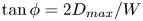 $\tan \phi = 2 D_{max} / W$, and solving for
  $\tan \phi$ in (C6), we retrieve (5.12) of § 5.3.
If we specify the full shape of the channel, we can find the integration constant,  $A$. In a triangular channel of figure 9(a), the depth profile is given by
 \begin{equation} \tilde{D} = \begin{cases} \tilde{y} \tan \phi & \text{if } \tilde{y} \leq \dfrac{\tilde{W}}{2}, \\ (\tilde{W} - \tilde{y}) \tan \phi & \text{if } \tilde{y} > \dfrac{\tilde{W}}{2}. \end{cases} \end{equation}
In both halves of the channel the solution is given by the same sum of the particular and homogeneous solution we just discussed, so we simply need to determine the constant,  $A$. To find it, we assume that the stress,
  $\tau\!$, and the flux,
  $F$, are continuous at the junction between the two halves (in fact, due to symmetry, the flux at this point vanishes). This yields
 \begin{equation} A = \frac{\tilde{D}_{max}^{1-a}}{(2\alpha+a) (2\chi\left( \tan \phi \right)^2 - \sqrt{1 + \left( \tan \phi \right)^2}/(2\alpha + 1))} . \end{equation}
These solutions are shown in figure 9(b,c).
C.1. Poisson equation
To find the unapproximated laminar stress in the triangular channel of figure 9 (red dotted line in figure 9), we solve the Poisson equation for the velocity,
 \begin{equation} \frac{\partial^2 \tilde{u}}{\partial \tilde{y}^2} + \frac{\partial^2 \tilde{u}}{\partial \tilde{z}^2} =-1 , \end{equation}
with a no-slip boundary condition at the bed,  $\tilde {u}(\tilde {z} = -\tilde {D}) = 0$. Since this equation is linear, the resulting velocity is the sum of the particular and the homogeneous solution,
  $\tilde {u} = \tilde {u}_{p} + \tilde {u}_{h}$. For the corner of (C1), the particular solution is
 \begin{equation} \tilde{u}_{p} = \frac{ (\tilde{y} \tan \phi )^2 - \tilde{z}^2 }{2 (1 - \tan^2 \phi)} . \end{equation}
A homogeneous solution is (Polubarinova-Kochina Reference Polubarinova-Kochina1962)
 \begin{equation} \tilde{u}_{h} = C_n {Re}\left( \omega^{(2n+1) ({\rm \pi}/{2\phi})} \right) \end{equation}
for any integer  $n > 0$. Here,
  $\omega = \tilde {y} + i \tilde {z}$ is a complex combination of the coordinates,
  ${Re}( \cdots )$ stands for the real part and
  $C_n$ is a constant. Therefore, the full solution,
  $\tilde {u}$, is
 \begin{equation} \tilde{u}(\tilde{y}, \tilde{z}) = \frac{ (\tilde{y} \tan \phi )^2 - \tilde{z}^2 }{2 (1 - \tan^2 \phi)} + \sum_{n=1}^{\infty} C_n {Re}(\omega^{(2n+1) ({\rm \pi}/{2\phi})}) , \end{equation}
where  $C_n$ are constants to be determined from the boundary condition at the centre of the triangular channel. Due to the symmetry of the channel, the velocity gradient must vanish at the centre,
  $\partial \tilde {u} / \partial \tilde {y} |_{\tilde {y} = \tilde {W}/2} = 0$. By considering this condition at
  $N$ distinct heights,
  $\tilde {z}_1 \mathrm {,\ldots,} \tilde {z}_N$, we can find the constants
  $C_n$ to arbitrary order
  $N$ (the solution in figure 9 assumes
  $N = 50$). After determining the constants
  $C_n$, we find the components of the stress as
  $\tilde {\tau }_z = \partial \tilde {u} / \partial \tilde {z} |_{\tilde {z} = -\tilde {D}}$ and
  $\tilde {\tau }_y = \partial \tilde {u} / \partial \tilde {y} |_{\tilde {z} = -\tilde {D}}$, and the total stress as
  $\tilde {\tau } = (\tilde {\tau }_z^2 + \tilde {\tau }_y^2 )^{1/2}$.
Appendix D. Details about the experiments
In this appendix we give the details of the experiments we compared our model with. All of these details can be found in the cited references, but we give them here for the reader's convenience.
D.1. Chauvet et al. (Reference Chauvet, Devauchelle, Métivier, Lajeunesse and Limare2014)
In the Paris region, the Seine river flows down a gentle slope of about  $S \approx 10^{-4}$, with a Reynolds number of about
  ${Re} \approx 7 \times 10^6$. At the time and the location at which Chauvet et al. (Reference Chauvet, Devauchelle, Métivier, Lajeunesse and Limare2014) took their measurements, it was about
  $148\ \text {m}$ wide and about
  $6.2\ \text {m}$ deep. Their measurements were based on readings from an acoustic doppler current profiler fixed to a raft that was tethered to a footbridge, and shifted across the flow.
D.2. Knight et al. (Reference Knight, Demetriou and Hamed1984)
Knight et al. (Reference Knight, Demetriou and Hamed1984) performed a series of experiments in smooth rectangular channels whose width varied between  $W =7\ \text {cm}$ and
  $W = 61\ \text {cm}$. The slope in all experiments was fixed at
  $S = 9.66\times 10^{-4}$, while the flow depth was varied by adjusting the water discharge. The resulting aspect ratio varied between
  $0.31$ and
  $19.12$, with a Reynolds number varying between about
  $10^4$ and
  $7\times 10^4$. They measured the stress with a Preston tube method (Preston Reference Preston1954).
D.3. Shiono & Knight (Reference Shiono and Knight1991)
Shiono & Knight (Reference Shiono and Knight1991) investigated the flow and the stress distribution in idealised experiments that resemble a river with a floodplain (figure 13). Their channels consisted of a deep main channel of width  $W_{mc} = 1.5\ \text {m}$, surrounded by two shallow parts (the ‘floodplain’), each
  $W_{fp} = 2.25\ \text {m}$ wide. The water level changed from one experiment to the next, so that the depth of the main channel varied between
  $D_{mc} = 15\ \text {cm}$ and
  $D_{mc} = 30\ \text {cm}$, and that of the floodplain between
  $D_{fp} = 0$ and
  $D_{fp} = 15\ \text {cm}$. The difference between the two depths was fixed by experimental design at
  $D_{mc} - D_{fp} = 15\ \text {cm}$. The downstream slope of the channel was fixed at
  $S = 1.027\times 10^{-3}$. Shiono & Knight (Reference Shiono and Knight1991) measured the velocity using a two-channel laser doppler anemometer across one half of the channel. They measured the stress across the channel using Preston tubes (Preston Reference Preston1954). The velocities were about
  $1\ \text {m}\ \text {s}^{-1}$, which yields a Reynolds number of about
  $3\times 10^5$, similar to the largest experiments considered by Knight et al. (Reference Knight, Demetriou and Hamed1984), and about an order of magnitude lower than in the Seine.
D.4. Blanckaert et al. (Reference Blanckaert, Duarte and Schleiss2010)
The experiments of Blanckaert et al. (Reference Blanckaert, Duarte and Schleiss2010) were performed in half-trapezoidal channels, such as the one shown in figure 14. The left bank was a vertical wall, whereas the right bank had a slope of either  $30^\circ$ or
  $45^\circ$, depending on the experiment. The width of the flat bottom was about
  $W_{bot}= 1.2 \ \text {m}$, the flow depth about
  $D_{bot} = 16 \ \text {cm}$, the flow speed about
  $U\sim 0.4 \ \text {m}\ \text {s}^{-1}$ and the Reynolds number about
  ${Re} \sim 7\times 10^4$. The bottom of the channel was roughened by gluing beads of size
  $k_{s, {bot}} = 2\ \text {mm}$. They considered three cases for the banks: smooth banks (
 $k_{s, {bank}} \approx 0$), banks that were as rough as the bottom (
 $k_{s, {bank}} = 2 \ \text {mm}$) and rough banks (
 $k_{s, {bank}} = 30 \ \text {mm}$). Unlike Shiono & Knight (Reference Shiono and Knight1991), Blanckaert et al. (Reference Blanckaert, Duarte and Schleiss2010) did not measure the stress directly, but estimated it from the vertical velocity profiles.


