


1. Introduction
This study concerns the fluid motion induced by a rigid circular disk (or piston) of radius  $a$ vibrating along its axis in the vicinity of a stationary parallel surface. The three specific geometrical configurations to be analysed are represented in figure 1. The width of the gap separating the two parallel surfaces varies harmonically in time according to
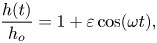 \begin{equation} \frac{h(t)}{h_o}=1+\varepsilon \cos(\omega t), \end{equation}
where  $h_o \ll a$ is the mean separation distance, $\omega$ is the angular frequency and $\varepsilon h_o$ is the oscillation amplitude, with $\varepsilon \ll 1$ in our study. Such slender-flow systems, commonly referred to as squeeze films, are of great interest in the context of gas lubricated bearings present in high-speed rotary machinery and also in acoustic levitation devices used in assembly line transport of microelectronics (see Shi et al. Reference Shi, Feng, Hu, Zhu and Cui2019). In the former case of squeeze-film air bearings, there is great demand for predicting the load capacity, while in the latter, referred to as near-field acoustic levitation, the sensitivity of transported items additionally warrants comprehension of radial pressure departures $p-p_a$ from the outer ambient value $p_a$. A key aspect of the problem is that, although the disk motion is harmonic, the resulting overpressure $p-p_a$ displays, in general, a non-zero time-averaged value at any given location, which is a consequence of the inherent nonlinearities introduced by convection and gas compressibility. As a result, the disk or piston experiences a steady perpendicular force, typically referred to as the time-averaged ‘squeeze-film force’.
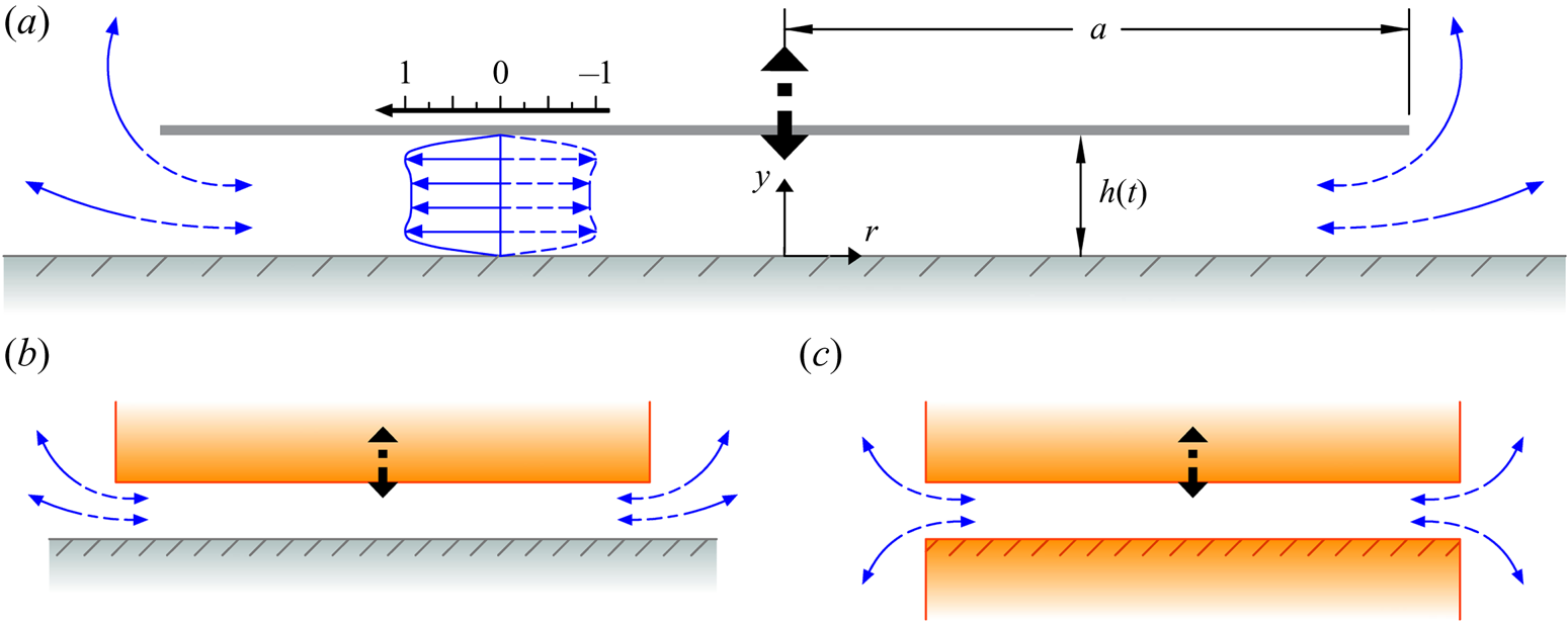
Figure 1. Schematic illustration of the three axisymmetric flow configurations examined in this study, including (a) a disk or (b) a piston vibrating close to an infinite wall and (c) a piston vibrating close to another piston. The curved arrows in each case represent the edge flow region, extending over radial distances  $r-a \sim h_o$. The velocity profile pictured inside the slender inner region $a \geqslant a-r \gg h_o$ of the disk–wall configuration in panel (a) corresponds to the leading-order flow (4.11) generated for a Stokes number of $\alpha ^2=300$.
Analysis of the fluid flow induced by the disk oscillations must consider the existence of two different regions, namely, the slender film separating the disk from the planar wall at radial distances  $r$ in the range $a \geqslant a-r \gg h_o$, where streamlines are aligned with the parallel surfaces, and the non-slender edge region that extends over distances of order $h_o$ from the disk edge, which controls the exchange of fluid with the surrounding stagnant atmosphere and its associated pressure drop. We shall see that the character of the flow in the slender film depends on the characteristic oscillation time $\omega ^{-1}$, which is to be compared with the two relevant mechanical times, namely, the viscous time across the gas layer $t_v=h_o^2/(\mu _a/\rho _a)$, where $\mu _a$ and $\rho _a$ are the values of the viscosity and density in the surrounding atmosphere, and the characteristic acoustic time for radial-pressure equilibration $t_a=a/(p_a/\rho _a)^{1/2}$, where $(p_a/\rho _a)^{1/2}$ is, aside from a factor $\gamma ^{1/2}$, the ambient value of the sound speed, with $\gamma$ denoting the ratio of specific heats. The analysis that follows assumes all three times to be comparable, yielding order-unity values of the Stokes number
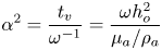 \begin{equation} \alpha^2=\frac{t_v}{\omega^{{-}1}}= \frac{\omega h_o^2}{\mu_a/\rho_a} \end{equation}
and of the compressibility parameter
 \begin{equation} \varLambda=\left(\frac{t_a}{\omega^{{-}1}} \right)^{2}=\frac{\omega^2 a^2}{p_a/\rho_a}. \end{equation}
The three length scales present in the problem (i.e. the disk radius  $a$, the mean separation distance $h_o$ and the oscillation amplitude $\varepsilon h_o$) introduce two additional operational parameters – the relative oscillation amplitude $\varepsilon$ and the slenderness ratio $\delta =h_o/a \ll 1$. It will be shown in the following analysis that the time-averaged pressure drop across the slender film, identical for all three geometrical configurations shown in figure 1, depends solely on $\alpha ^2$ and $\varLambda$, while that across the edge region, different for each geometrical configuration, depends additionally on a third controlling parameter, the local Strouhal number
 \begin{equation} {\textit{St}} = \frac{t_c}{\omega^{{-}1}} = \frac{\delta}{\varepsilon} , \end{equation}
where  $t_c=h_o/(\varepsilon \omega a)$ is the characteristic residence time in the edge region. The majority of previous analyses of squeeze-film systems $\delta \ll 1$ have been restricted to specific limiting cases of the slender gas-film problem, arising for extreme values of $\alpha ^2$ and $\varLambda$, namely, incompressible flow for $\varLambda \ll 1$, inviscid flow for $\alpha ^2 \gg 1$ and lubrication flow for $\alpha ^2 \ll 1$. A unifying viscoacoustic theory of squeeze-film systems, which embodies all of these specific cases and accounts for the pressure variation across the edge region, is to be developed here by considering the regime $\alpha ^2 \sim 1$ and $\varLambda \sim 1$ for asymptotically small values of the relative oscillation amplitude $\varepsilon \ll 1$ and the slenderness ratio $\delta \ll 1$ in the distinguished limit $\varepsilon \sim \delta$ (or equivalently $St\sim 1$). It is worth noting that, because the mean free path is of order $\ell \sim (\mu _a/\rho _a)/(p_a/\rho _a)^{1/2}$, in the limit investigated here, the relevant Knudsen number in the gas layer is $\ell /h_o \sim (\varLambda ^{1/2}/\alpha ^2) (h_o/a) \sim \delta \ll 1$, thereby guaranteeing applicability of the continuum hypothesis to the description of the flow.
The lubrication limit  $\alpha ^2 \ll 1$, corresponding to negligible fluid acceleration, has been widely studied throughout the twentieth century by way of the isothermal squeeze-film equations, a subclass of the well-known Reynolds lubrication equation tailored for modelling squeeze-film bearings of various geometries (see Reynolds Reference Reynolds1886). Specific interest in the role of compressibility in the slender gas layer was piqued by an experiment conducted by Popper & Reiner (Reference Popper and Reiner1956), where a disk rotating around its axis in close proximity to a parallel wall was reported to experience a perpendicular suction force that transitioned to growing repulsion as the gap between the disk and the wall was reduced. In a subsequent clarifying analysis, Taylor & Saffman (Reference Taylor and Saffman1957) proved that the observed repulsive squeeze-film force could be explained by effects of compressibility arising from imperfections in the operation of the rotor such as off-axis rotation or normal vibrations. They demonstrated using perturbation methods that the steady overpressure resulting from the latter case scales with the square of the dimensionless vibration amplitude $\varepsilon$ and depends on a single parameter – the squeeze number $\sigma =12\varLambda /\alpha ^2$. These results were formalized by Langlois (Reference Langlois1962) in the context of the classical squeeze-film equations for planar and axisymmetric geometries. Finite-difference solutions of the axisymmetric squeeze-film equation were experimentally verified by Salbu (Reference Salbu1964), who noted the presence of a central region dominated by viscous damping where the film pressure is effectively uniform and a near-edge region where the pressure drops to ambient conditions, the latter of which was treated by DiPrima (Reference DiPrima1968) as a mathematical boundary layer of thickness $O(\sigma ^{-1/2})$. Ideal squeeze-film lubrication theory, wherein the pressure at the edge of the film can be considered equal to the ambient pressure, was later proven invalid for diminishing values of $\sigma$ by Minikes & Bucher (Reference Minikes and Bucher2006), who determined numerically that imposing instead a non-reflective radiation boundary condition at the edge, allowing acoustic energy leakage, caused a relative reduction of approximately $50\,\%$ in the predicted film force.
One of the first clarifying analyses of the role of fluid inertia in incompressible squeeze films  $\varLambda \ll 1$ was contributed by Terrill (Reference Terrill1969), who determined the time-dependent overpressure in the gas layer for asymptotically small values of the inner Reynolds number $\alpha ^2\varepsilon$. Following this work, a number of studies have been conducted to account for time-averaged pressure corrections introduced by convective acceleration in the near-edge region (see, for example Hori Reference Hori2006), including a recent model proposed by Li et al. (Reference Li, Cao, Liu and Ding2010) that employs an approximate boundary condition at the edge of the gas layer, yielding satisfactory agreement with experimental results (i.e. the time-averaged overpressure at $r=a$ contributed by downward strokes of the disk oscillation is assumed to be zero and that contributed by upward strokes is estimated by applying integral conservation laws to a control volume extending an arbitrary distance from the edge).
The limit of large Stokes numbers  $\alpha ^2 \gg 1$, where the flow is nearly inviscid outside thin near-wall boundary layers, has been the subject of widespread interest in the context of acoustic levitation, which typically concerns the suspension of light objects in the antinodes of standing pressure waves between a vibrating piston and a reflector plate separated by an integral multiple of the half-wavelength of sound (see Shi et al. Reference Shi, Feng, Hu, Zhu and Cui2019). In 1902, Lord Rayleigh presented a foundational formulation of acoustic radiation inside a cylindrical piston of air undergoing transverse vibrations, expressing the overpressure in terms of the volumetric energy density (see Rayleigh Reference Rayleigh1902). After several years of disagreement over the application of Rayleigh's theory to acoustic levitation, Chu & Apfel (Reference Chu and Apfel1982) detailed the one-dimensional Rayleigh and Langevin radiation pressures – for flows with and without radial confinement – imposed by a vibrating piston on a perfectly reflecting parallel surface for arbitrary mean separation width. Clarifications were provided regarding distinctions between the Eulerian and Lagrangian definitions of the time average, the role played by second–order acoustic straining in reducing the mean pressure and the additional hydrostatic pressure contributed by edge flow confinement. Experimental verification of their theory was provided by Ueha, Hashimoto & Koike (Reference Ueha, Hashimoto and Koike2000), who demonstrated that when the mean separation width is small enough to deter interference of transverse acoustic waves, the reflector plate itself may experience repulsive forces of the order of 100 N. Sadayuki (Reference Sadayuki2002) experimentally demonstrated the onset of weak adhesive forces below critical vibration frequencies, a finding that was substantiated computationally by Andrade et al. (Reference Andrade, Ramos, Adamowski and Marzo2020). Their direct numerical simulations, which assumed isentropic flow, helped clarify that the transition from levitation to adhesion is caused by steady negative overpressures near the edge of the slender gas layer becoming comparable to the positive inner contributions.
While the limits of lubrication theory and acoustic levitation are accurate for small and large values of  $\alpha =h_o/[\mu _a/(\rho _a \omega )]^{1/2}$, respectively, neither is valid for bearings with mean film widths $h_o$ comparable to the thickness of the viscous shear layers $[\mu _a/(\rho _a \omega )]^{1/2}$. Practical applicability of either theory in hydrodynamic bearings is further complicated because equilibrium separation distances are typically unknown prior to operation, which yields uncertainty in the choice of the needed analytical framework. Melikhov et al. (Reference Melikhov, Chivilikhin, Amosov and Jeanson2016) addressed this problem by numerically computing the levitation force for a compressible squeeze-film system with arbitrary Stokes number. In determining the time-averaged pressure distribution across the slender film, Melikhov et al. (Reference Melikhov, Chivilikhin, Amosov and Jeanson2016) imposed a Robin boundary condition that enforces strictly acoustic wave propagation at its edge, which yielded a model that demonstrates reasonable agreement between theoretically predicted and experimentally determined levitation heights $h_o$. To the best of our knowledge, a complete viscoacoustic theoretical analysis of the axisymmetric squeeze-film problem that accounts for the existence of the edge flow region is yet to be developed. Such analysis, which is the objective of the present paper, is needed to delineate precisely the parametric conditions associated with transition from repulsive to attractive forces.
The limit  $\varLambda \sim 1$, $\alpha ^2 \sim 1$ and $\varepsilon \sim \delta \ll 1$ addressed herein enables the analysis of effects of local acceleration, viscous dissipation, thermal diffusion, acoustic wave propagation and nonlinearities introduced by convection and compressibility, while encompassing the specific cases investigated in the past as limiting solutions for extreme values of the controlling parameters $\varLambda$ and $\alpha ^2$. The method of matched asymptotic expansions will be used to relate the solution in the two distinct flow regions, ultimately providing quantitative information regarding the dependence of the time-averaged force on the governing parameters $\varLambda$, $\alpha ^2$ and ${\textit {St}}=\delta /\varepsilon$, and the specific edge geometry (see figure 1). The squeeze-film force will be shown to involve two comparable contributions – the first accounting for variations of the pressure across the slender gas layer from its value at the edge $r=a$ and the second involving the pressure drop across the near-edge region from said value to ambient conditions.
The remainder of this paper is organized as follows. The reduced conservation equations governing each of the two distinct flow regions are presented in § 2 in dimensional form, accompanied by justificatory discussions of the associated characteristic scales. The dimensionless conservation equations pertaining to the slender inner region are written in § 3 and their leading-order time-harmonic solution is presented in § 4. Associated first-order corrections to the film pressure are computed in § 5 and used to determine the first contribution to the time-averaged levitation force, along with simplified expressions of both for limiting values of the Stokes number and the compressibility parameter. The dimensionless conservation equations describing flow in the edge region of the squeeze film are written in § 6, supplemented by a boundary condition that accounts for the driving radial velocity present at the edge of the slender gas film, obtained by asymptotically matching with the leading-order inner solution. Numerical computations of the time-averaged pressure drop across the edge region are presented, along with predictions of its behaviour for limiting values of the Stokes number and the edge Strouhal number. The dependence of the steady squeeze-film force acting on the oscillating body – which accounts for comparable pressure contributions from the two distinct flow regions – on the three governing parameters is discussed in § 7 with specific attention dedicated to the criteria required for a transition between levitative and adhesive forces. The force predicted by our asymptotic analysis is compared with that determined in the recent direct numerical simulations of Andrade et al. (Reference Andrade, Ramos, Adamowski and Marzo2020). Closed form analytical expressions facilitatory for low-cost computation of the steady film pressure and squeeze-film force are provided in an appendix, and finally, concluding remarks are given in § 8.
Our asymptotic analysis: (i) reveals that the time-averaged pressure variations across the edge region are comparable in magnitude and opposite in sign to those found along the wall-bounded gas layer; (ii) leads to simplified expressions that expedite the evaluation of the steady squeeze-film force over a wide range of conditions of practical interest, facilitating the operation and control of high-frequency systems; (iii) unveils a boundary on the  $\alpha ^2-\varLambda$ parametric plane across which the force switches from repulsion to attraction; (iv) demonstrates numerically that the force is only weakly dependent on the specific geometrical configuration and (v) compares favourably with recently published computational results (see Andrade et al. Reference Andrade, Ramos, Adamowski and Marzo2020).
2. Distinct regions and characteristic scales
An asymptotic analysis of the flow induced by the harmonic disk oscillations defined in (1.1) is to be given for  $\alpha ^2 \sim 1$ and $\varLambda \sim 1$ in the distinguished double limit $\varepsilon \ll 1$ and $\delta =h_o/a \ll 1$ with $\varepsilon \sim \delta$. The axisymmetric periodic motion will be described in terms of the radial and axial velocity components $u(r,y,t)$ and $v(r,y,t)$, with $y$ and $r$ denoting the axial distance from the wall and the radial distance from the disk centre, as indicated in figure 1. The description must account for the variations of the pressure $p$, density $\rho$ and temperature $T$ of the gas from their ambient values $p_a$, $\rho _a$ and $T_a$. The analysis must consider the existence of two distinct regions, namely, the slender gas layer separating the disk from the planar wall, where the streamlines are nearly parallel to the bounding solid surfaces, and the boundary region of non-slender flow extending over distances of order $h_o$ from the disk edge. We shall give below the reduced conservation equations and the associated scales for the flow in these two regions.
The full compressible Navier–Stokes equations governing the axisymmetric flow investigated here can be found in Schlichting & Gersten (Reference Schlichting and Gersten2016) in cylindrical form. In the slender gas film separating the two parallel solid surfaces, where  $r\sim a$ and $y\sim h_0 \ll a$, these conservation equations can be simplified to the boundary-layer form
 $$\begin{gather} \frac{\partial \rho}{\partial t} +\frac{1}{r} \frac{\partial}{\partial r}(\rho ru)+\frac{\partial }{\partial y}(\rho v) =0 , \end{gather}$$
 $$\begin{gather}\frac{\partial p}{\partial y} = 0 , \end{gather}$$
 $$\begin{gather}\rho \left( \frac{\partial u}{\partial t}+u \frac{\partial u}{\partial r}+v \frac{\partial u}{\partial y}\right)={-}\frac{\partial p}{\partial r} +\frac{\partial}{\partial y} \left(\mu \frac{\partial u}{\partial y} \right), \end{gather}$$
 $$\begin{gather}\rho c_p \left( \frac{\partial T}{\partial t}+u \frac{\partial T}{\partial r}+v \frac{\partial T}{\partial y}\right)-\left(\frac{\partial p}{\partial t}+u \frac{\partial p}{\partial r}\right)=\mu \left(\frac{\partial u}{\partial y}\right)^2+\frac{\partial}{\partial y} \left( \kappa \frac{\partial T}{\partial y}\right) . \end{gather}$$
For the slender flow analysed here, molecular-transport terms involving radial derivatives are a factor  $(h_o/a)^2=\delta ^2 \ll 1$ smaller than those involving transverse derivatives, so that only the latter have been retained in writing the viscous force per unit volume in (2.3) and the heat-conduction and viscous-dissipation terms in (2.4). At the same level of approximation (i.e. with small relative errors of order $\delta ^2 \ll 1$), the analysis neglects the variations of the pressure across the gas layer, as reflected by the reduced equation (2.2). In the proceeding analysis, the specific heat at constant pressure $c_p$ is assumed to be constant, while the viscosity coefficient $\mu$ and the thermal conductivity $\kappa$ are assumed to vary from their ambient values according to $(\mu /\mu _a) = (\kappa /\kappa _a) = (T/T_a)^\nu$ with $\nu \approx 0.77$, an excellent approximation for air (Chapman & Cowling Reference Chapman and Cowling1990), for which the Prandtl number takes the value ${\textit {Pr}}=c_p \mu /\kappa =0.7$ and the ratio of specific heats takes the value $\gamma =1.4$. The above equations must be supplemented with the equation of state
 \begin{equation} \frac{p}{p_a}=\frac{\rho}{\rho_a} \frac{T}{T_a}. \end{equation}
 In the slender gas layer, the axial velocities induced by the displacement rate  ${\textrm {d} h}/{\textrm {d} t}=-\varepsilon \omega h_o \sin (\omega t)$ of the moving surface are of order $v_c=\varepsilon \omega h_o$. The associated radial velocities are much larger, of order $u_c=v_c/\delta =\varepsilon \omega a$, as follows from the straightforward order-of-magnitude balance $u_c/a \sim v_c/h_o$ stemming from (2.1). Since it is assumed that the characteristic time for the oscillatory motion $\omega ^{-1}$ is comparable to the characteristic viscous and heat conduction times across the gaseous film $t_v=h_o^2/(\mu _a/\rho _a)$ and $t_h={\textit {Pr}} \, t_v \sim t_v$, viscous stresses and heat conduction can be expected to have, in general, a significant effect on the oscillatory flow. In contrast, convective acceleration has a negligible effect at leading order in the limit $\varepsilon \ll 1$, because the associated Strouhal number is $\varepsilon ^{-1} \gg 1$, as can be seen by comparing the orders of magnitude of the local acceleration $\partial u/\partial t\sim \omega u_c$ and the convective acceleration $u\:\partial u/\partial r\sim u_c^2/a$ in (2.3). A similar order-of-magnitude analysis in the energy equation (2.4) provides $(u \partial T/\partial r)/(\partial T/\partial t) \sim \varepsilon$, indicating that convective heat transport is also negligible at leading order. Note that since the characteristic value of the radial pressure variations $p-p_a$ needed to produce velocity changes of order $u_c=\varepsilon \omega a$ in times of order $\omega ^{-1}$ is $\Delta p = \rho _a \varepsilon \omega ^2 a^2$, as follows from the balance $\partial p/\partial r \sim \rho \,\partial u/\partial t$, the resulting instantaneous levitation force acting on the disk is expected to be of order $\mathcal{F}_l \sim \Delta p \, a^2 = \rho _a \varepsilon \omega ^2 a^4$.
In the limit  $\varLambda \sim 1$ considered here, the pressure variations $p-p_a \sim \Delta p$ induced in the gap are small compared with the ambient pressure, as can be seen by writing $\Delta p/p_a \sim \varepsilon (\omega ^2 a^2)/(p_a/\rho _a)=\varepsilon \varLambda$. Correspondingly, the relative density and temperature variations from their respective ambient values are also small, of order $(\rho -\rho _a)/\rho _a \sim (T-T_a)/T_a \sim \varepsilon \varLambda$, as follows from the equation of state (2.5). The conservation equations (2.1)–(2.5) at leading order will be shown to reduce to a linear problem describing compressible unsteady lubrication flow, which will be solved analytically in closed-form. The leading-order flow variables will be shown to vary harmonically with time, thus yielding no time-averaged contributions over a period of the driving oscillations, with the time-averaging operator formally defined by
 \begin{equation} \langle \cdot \rangle = \frac{\omega}{2{\rm \pi}} \int_t^{t+2 {\rm \pi}/\omega} \cdot \, \textrm{d}t . \end{equation}
We shall see that because the pressure distribution at leading order has a zero time-averaged value, the computation of the time-averaged levitation force  $\langle \mathcal{F}_l \rangle$ requires quantification of higher-order corrections associated with nonlinear convective and compressibility effects, which involve time-averaged pressure differences $\langle p-p_a \rangle$ of order $\rho _a \varepsilon ^2\omega ^2 a^2 = \varepsilon \Delta p$. The associated time-averaged levitation force $\langle \mathcal{F}_l \rangle \sim \varepsilon \Delta p \, a^2 = \varepsilon ^2 \rho _a \omega ^2 a^4$ can be expressed conveniently in dimensionless form as
 \begin{equation} \frac{\langle \mathcal{F}_l \rangle}{\varepsilon^2\rho_a\omega^2{\rm \pi} a^4} = \frac{2}{\varepsilon} \int_0^1 \frac{\langle p-p_a \rangle}{\Delta p} \frac{r}{a} \textrm{d}\left(\frac{r}{a}\right). \end{equation}
 The slender gas layer, where the radial velocity is of order  $u\sim u_c$, connects with the ambient atmosphere through a non-slender near-edge boundary region where $r-a \sim y \sim h_o$ and $u \sim v \sim u_c$. The flow in this region involves small pressure variations of order $(p-p_a)/p_a \sim \varepsilon ^2\varLambda$, as follows from a balance between the pressure force per unit mass $\rho ^{-1} \boldsymbol {\nabla } p \sim (p-p_a)/(\rho _a h_o)$ and the convective acceleration $\boldsymbol {v} \boldsymbol {\cdot } \boldsymbol {\nabla } \boldsymbol {v} \sim u_c^2/h_o$, with $\boldsymbol {v}=(u,v)$ and $\boldsymbol {\nabla }=(\partial /\partial r,\partial /\partial y)$. As can be expected from the equation of state (2.5), the associated density and temperature variations in this region are also small, of order $(\rho -\rho _a)/\rho _a \sim (T-T_a)/T_a \sim (p-p_a)/p_a \sim \varepsilon ^2\varLambda$, so that at leading order in the limit $\varepsilon \ll 1$, the flow is effectively incompressible and features constant transport properties. Also, because $r-a \sim y \sim h_o \ll a$, the leading-order flow is locally planar, with a velocity field determined from the familiar incompressible two-dimensional equations
 $$\begin{gather} \boldsymbol{\nabla} \boldsymbol{\cdot} \boldsymbol{v} = 0 , \end{gather}$$
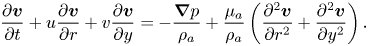 $$\begin{gather}{\frac{\partial \boldsymbol{v}}{\partial t}} + u{\frac{\partial \boldsymbol{v}}{\partial r}}+v{\frac{\partial \boldsymbol{v}}{\partial y}} ={-}\frac{\boldsymbol{\nabla} p}{\rho_a} + \frac{\mu_a}{\rho_a} \left(\frac{\partial^2 \boldsymbol{v}}{\partial r^2}+\frac{\partial^2 \boldsymbol{v}}{\partial y^2} \right) . \end{gather}$$
Using  $u \sim v \sim u_c=\varepsilon \omega a$ in (2.9) provides the orders of magnitude of the local acceleration $\partial \boldsymbol {v}/\partial t \sim \omega u_c$, convective acceleration $\boldsymbol {v} \boldsymbol {\cdot } \boldsymbol {\nabla } \boldsymbol {v} \sim u_c^2/h_o$ and viscous force per unit mass $(\mu _a/\rho _a) \nabla ^2\boldsymbol {v} \sim (\mu _a/\rho _a) u_c/h_o^2$, giving values that are comparable in magnitude in the limit $\alpha ^2 \sim 1$ considered here, so that all terms in (2.9) must, in general, be retained in the description. It will be shown that the pressure drop across this boundary region, of order $p-p_a \sim \rho _a \varepsilon \omega ^2 a h_o= \delta \Delta p$, contains a non-zero time-averaged component. In the distinguished limit $\delta \sim \varepsilon$, this local pressure drop is comparable in magnitude to the time-averaged pressure differences $\langle p-p_a \rangle \sim \varepsilon \Delta p$ induced along the gas film and must therefore be accounted for in computing the steady levitation force, as done in the following perturbation analysis.
The asymptotic analysis will consider separate solutions in the slender gas layer and in the near-edge region. The scales identified above will be used in defining appropriate dimensionless variables of order unity in each region. Following standard practice (see Lagerstrom Reference Lagerstrom1988), asymptotic expansions in increasing powers of  $\varepsilon$ will be introduced for the different flow variables, leading to a hierarchy of problems that will be solved sequentially with account taken of the matching conditions arising at each order. To compute the time-averaged levitation force (2.7) with small relative errors of order $\varepsilon \sim \delta$, the description must consider two terms in the expansions for the slender region, whereas only the leading-order terms are needed in the near-edge region.
3. Formulation of the problem in the slender gaseous film
The analysis uses the dimensionless time  $\tau =\omega t$ and dimensionless gap width
 \begin{equation} H=\frac{h}{h_o}=1+\varepsilon \cos(\tau) . \end{equation}
Substitution of the appropriate order-unity variables  $\xi =r/a$, $Y=y/h_o$, $U=u/u_c$, $V=v/v_c$, $P=(p-p_a)/\Delta p$, $R=(\rho -\rho _a)/(\varepsilon \varLambda \rho _a)$ and $\varTheta =(T-T_a)/(\varepsilon \varLambda T_a)$ into the governing equations (2.1) and (2.3)–(2.5) gives, with errors of order $\delta ^2 \sim \varepsilon ^2$,
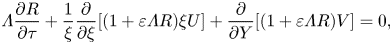 \begin{gather} \varLambda \frac{\partial R}{\partial \tau}+ \frac{1}{\xi} \frac{\partial}{\partial \xi} [(1+\varepsilon \varLambda R) \xi U]+\frac{\partial}{\partial Y}[(1+\varepsilon \varLambda R)V] =0, \end{gather}
 \begin{gather} (1+\varepsilon \varLambda R) \left[\frac{\partial U}{\partial \tau}+\varepsilon \left( U \frac{\partial U}{\partial \xi}+V \frac{\partial U}{\partial Y} \right)\right]={-} \frac{\partial P}{\partial \xi} +\frac{1}{\alpha^2} \frac{\partial}{\partial Y} \left[(1+\varepsilon \varLambda \varTheta)^\nu \frac{\partial U}{\partial Y}\right],\end{gather}
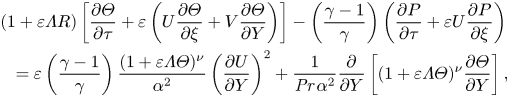 \begin{gather} (1+\varepsilon \varLambda R) \left[\frac{\partial \varTheta}{\partial \tau}+\varepsilon \left( U \frac{\partial \varTheta}{\partial \xi}+ V \frac{\partial \varTheta}{\partial Y} \right)\right]-\left(\frac{\gamma-1}{\gamma}\right) \left(\frac{\partial P}{\partial \tau}+\varepsilon U \frac{\partial P}{\partial \xi} \right) \nonumber\\ \quad = \varepsilon \left(\frac{\gamma-1}{\gamma}\right) \frac{(1+\varepsilon \varLambda \varTheta)^\nu}{\alpha^2} \left(\frac{\partial U}{\partial Y}\right)^2 +\frac{1}{{\textit{Pr}} \, \alpha^2} \frac{\partial}{\partial Y} \left[(1+\varepsilon \varLambda \varTheta)^\nu \frac{\partial \varTheta}{\partial Y}\right], \end{gather}
 \begin{gather} P=R+\varTheta+\varepsilon \varLambda R\varTheta, \end{gather}
while the axial momentum equation (2.2) becomes  $\partial P/\partial Y=0$, whence $P=P(\xi,\tau )$. The present system of equations admits analytic periodic solutions that satisfy isothermal non-slip conditions at the bounding walls,
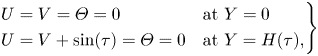 \begin{equation} \left. \begin{array}{ll@{}} U=V=\varTheta=0 & \textrm{at} \ Y=0 \\
U=V+\sin(\tau)=\varTheta=0 & \textrm{at} \ Y=H(\tau) ,
\end{array} \right\} \end{equation}
\begin{equation} \left. \begin{array}{ll@{}} U=V=\varTheta=0 & \textrm{at} \ Y=0 \\
U=V+\sin(\tau)=\varTheta=0 & \textrm{at} \ Y=H(\tau) ,
\end{array} \right\} \end{equation}
together with the regularity condition at the axis of symmetry, which implies that
 \begin{equation} U={\frac{\partial P}{\partial \xi}}={\frac{\partial R}{\partial \xi}}={\frac{\partial \varTheta}{\partial \xi}} = 0 \quad \textrm{at} \ \xi=0 . \end{equation}
The needed boundary condition for the pressure  $P$ at the edge of the gas layer (i.e. at $\xi =1$) is to be obtained from matching with the near-edge solution, as described in the following analysis. Substitution of the scaled variables into (2.7) yields
 \begin{equation} \langle F_l\rangle = \frac{2}{\varepsilon} \int_0^1 \langle P \rangle \xi \,\textrm{d} \xi \end{equation}
for the dimensionless levitation force  $\langle F_l\rangle =\langle \mathcal{F}_l \rangle /(\varepsilon ^2\rho _a\omega ^2{\rm \pi} a^4)$. For future reference, it is of interest to note that (3.2) can be integrated across the gas layer to give
 \begin{equation} \varLambda \frac{\partial}{\partial \tau} \left(\int_0^H R \,\textrm{d} Y \right)+ \frac{1}{\xi} \frac{\partial}{\partial \xi} \left(\xi \int_0^H (1+\varepsilon \varLambda R) U \,\textrm{d} Y \right)-\sin(\tau)=0, \end{equation}
with use made of the well-known Leibniz integral rule to exchange the time derivative and spatial integral involved in the first term. Computing the time average of (3.9) and integrating the result in the radial direction gives
 \begin{equation} \left\langle \int_0^H (1+\varepsilon \varLambda R) U \,\textrm{d} Y \right\rangle=0 \end{equation}
upon imposing the boundary condition  $U=0$ at $\xi =0$.
4. Leading-order solution in the gaseous film
The above problem is to be solved for  $\varepsilon \ll 1$ by substituting the expansions
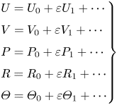 \begin{equation} \left. \begin{array}{l@{}}
U=U_0+\varepsilon U_1+\cdots \\ V=V_0+\varepsilon
V_1+\cdots \\ P=P_0+\varepsilon P_1+\cdots \\
R=R_0+\varepsilon R_1+\cdots \\
\varTheta=\varTheta_0+\varepsilon \varTheta_1+\cdots
\end{array} \right\} \end{equation}
\begin{equation} \left. \begin{array}{l@{}}
U=U_0+\varepsilon U_1+\cdots \\ V=V_0+\varepsilon
V_1+\cdots \\ P=P_0+\varepsilon P_1+\cdots \\
R=R_0+\varepsilon R_1+\cdots \\
\varTheta=\varTheta_0+\varepsilon \varTheta_1+\cdots
\end{array} \right\} \end{equation}
into (3.2)–(3.5) and solving sequentially the problems that arise at different orders in powers of  $\varepsilon$. Only the first two terms are to be considered in our analysis, consistent with the accuracy of (3.2)–(3.5) (note that the terms of order $\delta ^2 \sim \varepsilon ^2$ and smaller that were neglected in writing those equations would need to be retained if the analysis were to be carried out to higher orders).
To simplify the development, the axial coordinate  $Y$ will be replaced in the conservation equations (3.2)–(3.4) by its normalized counterpart $\eta =Y/H(\tau )$, with use of the substitutions, each accurate to order $\varepsilon$,
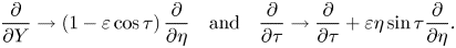 \begin{equation} {\frac{\partial }{\partial Y}} \to \left( 1-\varepsilon\cos\tau \right) {\frac{\partial }{\partial \eta}} \quad\textrm{and}\quad {\frac{\partial }{\partial \tau}} \to {\frac{\partial }{\partial \tau}} + \varepsilon\eta\sin\tau{\frac{\partial }{\partial \eta}} . \end{equation}
At leading order, the problem reduces to the integration of the linear system of equations,
 $$\begin{gather} \varLambda \frac{\partial R_0}{\partial \tau}+ \frac{1}{\xi} \frac{\partial}{\partial \xi} (\xi U_0)+\frac{\partial V_0}{\partial \eta}=0, \end{gather}$$
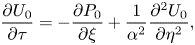 $$\begin{gather}\frac{\partial U_0}{\partial \tau}={-} \frac{\partial P_0}{\partial \xi} +\frac{1}{\alpha^2} \frac{\partial^2 U_0}{\partial \eta^2}, \end{gather}$$
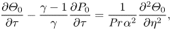 $$\begin{gather}\frac{\partial \varTheta_0}{\partial \tau}-\frac{\gamma-1}{\gamma} \frac{\partial P_0}{\partial \tau} = \frac{1}{{\textit{Pr}} \, \alpha^2} \frac{\partial^2 \varTheta_0}{\partial \eta^2}, \end{gather}$$
 $$\begin{gather}P_0=R_0+\varTheta_0, \end{gather}$$
subject to
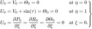 \begin{equation} \left.
\begin{array}{ll@{}} U_0=V_0=\varTheta_0=0 & \textrm{at} \
\eta=0 \\ U_0=V_0+\sin(\tau)=\varTheta_0=0 & \textrm{at} \
\eta=1 \\ U_0=\dfrac{\partial P_0}{\partial\xi}=\dfrac{\partial
R_0}{\partial\xi}=\dfrac{\partial\varTheta_0}{\partial\xi} = 0 & \textrm{at} \ \xi=0 . \end{array} \right\}
\end{equation}
\begin{equation} \left.
\begin{array}{ll@{}} U_0=V_0=\varTheta_0=0 & \textrm{at} \
\eta=0 \\ U_0=V_0+\sin(\tau)=\varTheta_0=0 & \textrm{at} \
\eta=1 \\ U_0=\dfrac{\partial P_0}{\partial\xi}=\dfrac{\partial
R_0}{\partial\xi}=\dfrac{\partial\varTheta_0}{\partial\xi} = 0 & \textrm{at} \ \xi=0 . \end{array} \right\}
\end{equation}
Because the pressure variation across the near-edge region is of order  $\delta \Delta p$, as described in the paragraph following (2.7), at leading order in the limit $\varepsilon \sim \delta \ll 1$, the pressure in the gap must satisfy
 \begin{equation} P_0= 0 \quad \textrm{at} \ \xi =1. \end{equation}
We shall see that the pressure drop across the near-edge region enters when matching with the following term in the expansion of the inner pressure, producing a non-zero first-order correction  $P_1 \ne 0$ at $\xi =1$ that must be accounted for when computing the time-averaged levitation force.
We begin the solution process by integrating (4.3) in the transverse direction using  $V_0(\eta =0)=0$, yielding
 \begin{equation} V_0(\eta) ={-}\int_0^\eta \left[ \varLambda{\frac{\partial R_0}{\partial \tau}} + \frac{1}{\xi}{\frac{\partial }{\partial \xi}}(\xi U_0) \right] \textrm{d}\eta , \end{equation}
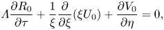
which will be useful later. Evaluating (4.9) at  $\eta =1$ gives
 \begin{equation} \int_0^1 \left[ \varLambda{\frac{\partial R_0}{\partial \tau}} + \frac{1}{\xi}{\frac{\partial }{\partial \xi}}(\xi U_0) \right] \textrm{d}\eta = \sin\tau , \end{equation}
which, along with (4.4)–(4.6), forms a closed system from which the four constituent variables  $P_0,\varTheta _0,R_0$ and $U_0$ can be fully determined. Because the leading-order problem in the gas layer (4.3)–(4.6) is linear and driven purely by time-harmonic boundary conditions (4.7), the five flow variables must necessarily vary harmonically with time. Additionally, it can be deduced from the discussion below (3.1) that the film pressure at this order does not vary in the transverse direction, that is,
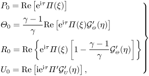
  $P_0=P_0(\xi,\tau )$. Upon consideration of these facts and close inspection of (4.4)–(4.6), we may anticipate that the solution can be expressed using separation of variables in the form
 \begin{equation} \left.\begin{array}{l@{}l}
P_0=\textrm{Re}\left[\mathrm{e}^{\mathrm{i} \tau}
\varPi(\xi) \right] \\ \varTheta_0=\dfrac{\gamma-1}{\gamma}
\textrm{Re}\left[\mathrm{e}^{\mathrm{i}\tau}\varPi(\xi)
\mathcal{G}_{\scriptscriptstyle{\varTheta}}'(\eta)\right] \\
R_0=\textrm{Re}\left\{\mathrm{e}^{\mathrm{i}\tau}\varPi(\xi)\left[1-\dfrac{\gamma-1}{\gamma}
\mathcal{G}_{\scriptscriptstyle{\varTheta}}'(\eta)\right]\right\}
\\
U_0=\textrm{Re}\left[\mathrm{i}\mathrm{e}^{\mathrm{i}\tau}\varPi'\mathcal{G}_{\scriptscriptstyle{U}}'(\eta)
\right] , \end{array} \right\}
\end{equation}
\begin{equation} \left.\begin{array}{l@{}l}
P_0=\textrm{Re}\left[\mathrm{e}^{\mathrm{i} \tau}
\varPi(\xi) \right] \\ \varTheta_0=\dfrac{\gamma-1}{\gamma}
\textrm{Re}\left[\mathrm{e}^{\mathrm{i}\tau}\varPi(\xi)
\mathcal{G}_{\scriptscriptstyle{\varTheta}}'(\eta)\right] \\
R_0=\textrm{Re}\left\{\mathrm{e}^{\mathrm{i}\tau}\varPi(\xi)\left[1-\dfrac{\gamma-1}{\gamma}
\mathcal{G}_{\scriptscriptstyle{\varTheta}}'(\eta)\right]\right\}
\\
U_0=\textrm{Re}\left[\mathrm{i}\mathrm{e}^{\mathrm{i}\tau}\varPi'\mathcal{G}_{\scriptscriptstyle{U}}'(\eta)
\right] , \end{array} \right\}
\end{equation}
where the transverse functions  $\mathcal{G}_{\scriptscriptstyle {U}}'(\eta )=\textrm {d}\mathcal{G}_{\scriptscriptstyle {U}}/\textrm {d}\eta$ and $\mathcal{G}_{\scriptscriptstyle {\varTheta }}'(\eta )=\textrm {d}\mathcal{G}_{\scriptscriptstyle {\varTheta }}/\textrm {d}\eta$ have been expressed as derivatives in anticipation of the integral in (4.9) necessary to determine $V_0$. Substituting (4.11) into (4.4) and (4.5) gives
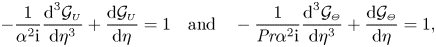 \begin{equation} -\frac{1}{\alpha^2\mathrm{i}} \frac{\textrm{d}^3\mathcal{G}_{\scriptscriptstyle{U}}}{\textrm{d} \eta^3}+\frac{\textrm{d} \mathcal{G}_{\scriptscriptstyle{U}}}{\textrm{d} \eta}=1 \quad\textrm{and}\quad -\frac{1}{{\textit{Pr}}\alpha^2\mathrm{i}} \frac{\textrm{d}^3\mathcal{G}_{\scriptscriptstyle{\varTheta}}}{\textrm{d} \eta^3}+\frac{\textrm{d} \mathcal{G}_{\scriptscriptstyle{\varTheta}}}{\textrm{d} \eta}=1, \end{equation}
respectively. Since the functions  $\mathcal{G}_{\scriptscriptstyle {U}}(\eta )$ and $\mathcal{G}_{\scriptscriptstyle {\varTheta }}(\eta )$ satisfy identical boundary conditions $\mathcal{G}_{\scriptscriptstyle {U}}'=\mathcal{G}_{\scriptscriptstyle {\varTheta }}'=0$ at $\eta =0,1$, as follows from (4.7), it is convenient to recast the above equations in the consolidated form
 \begin{equation} -\frac{1}{4\beta^2} \frac{\textrm{d}^3 \mathcal{G}}{\textrm{d} \eta^3}+\frac{\textrm{d} \mathcal{G}}{\textrm{d} \eta}=1 , \quad\textrm{with}\ \beta_{\scriptscriptstyle{U}}=\frac{\alpha}{2} \frac{(1+\mathrm{i})}{\sqrt{2}} \quad\textrm{and}\quad \beta_{\scriptscriptstyle{\varTheta}}=\sqrt{{\textit{Pr}}} \frac{\alpha}{2} \frac{(1+\mathrm{i})}{\sqrt{2}} , \end{equation}
where the function  $\mathcal {G}'(\eta ;\beta )=\textrm {d} \mathcal {G}/\textrm {d} \eta$ describes the transverse variations $\mathcal{G}_{\scriptscriptstyle {U}}'(\eta )=\mathcal {G}'(\eta ;\beta _{\scriptscriptstyle {U}})$ and $\mathcal{G}_{\scriptscriptstyle {\varTheta }}'(\eta )=\mathcal {G}'(\eta ;\beta _{\scriptscriptstyle {\varTheta }})$ of the radial velocity component and temperature deviation, respectively. The constant-coefficient ordinary differential equation in (4.13) can be integrated using (4.7) to give
 \begin{equation} \mathcal{G}=\eta-\frac{\sinh[\beta(2\eta-1)]+\sinh \beta}{2 \beta \cosh \beta} \quad \textrm{and} \quad \mathcal{G}'=1-\frac{\cosh[\beta(2\eta-1)]}{\cosh \beta} . \end{equation}
To determine the radial function  $\varPi (\xi )$, we substitute (4.11) and (4.14a,b) into (4.10), whereby we obtain the classical Bessel's equation
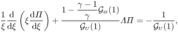 \begin{equation} \frac{1}{\xi} \frac{\textrm{d}}{\textrm{d} \xi}\left(\xi \frac{\textrm{d} \varPi}{\textrm{d}\xi} \right) + \frac{1-\dfrac{\gamma-1}{\gamma}\mathcal{G}_{\scriptscriptstyle{\varTheta}}(1)}{\mathcal{G}_{\scriptscriptstyle{U}}(1)} \varLambda \varPi={-}\frac{1}{\mathcal{G}_{\scriptscriptstyle{U}}(1)} , \end{equation}
which can be integrated using the boundary conditions  $\varPi (\xi =1)=\varPi '(\xi =0)=0$, consistent with (4.7), to give
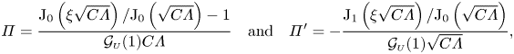 \begin{align} \varPi=\frac{\textrm{J}_0\left(\xi \sqrt{C \varLambda} \right)/\textrm{J}_0\left(\sqrt{C \varLambda}\right)-1}{\mathcal{G}_{\scriptscriptstyle U}(1) C \varLambda} \quad \textrm{and} \quad \varPi'={-}\frac{\textrm{J}_1\left(\xi \sqrt{C \varLambda}\right)/\textrm{J}_0\left(\sqrt{C \varLambda}\right)}{\mathcal{G}_{\scriptscriptstyle U}(1) \sqrt{C \varLambda}} , \end{align}
 where  $\textrm {J}_0$ and $\textrm {J}_1$ represent the Bessel functions of the first kind of order 0 and 1, respectively, and the constant $C$ is defined as
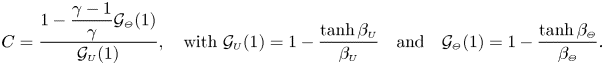 \begin{align} C= \frac{ 1-\dfrac{\gamma-1}{\gamma}\mathcal{G}_{\scriptscriptstyle{\varTheta}}(1) }{\mathcal{G}_{\scriptscriptstyle{U}}(1)} , \quad\textrm{with}\ \mathcal{G}_{\scriptscriptstyle{U}}(1) = 1 - \frac{\tanh\beta_{\scriptscriptstyle{U}}}{\beta_{\scriptscriptstyle{U}}} \quad\textrm{{and}}\quad \mathcal{G}_{\scriptscriptstyle{\varTheta}}(1) = 1 - \frac{\tanh\beta_{\scriptscriptstyle{\varTheta}}}{\beta_{\scriptscriptstyle{\varTheta}}} . \end{align}
The final step of the solution process is to substitute the known forms of  $U_0$ and $R_0$ into (4.9), which yields
 \begin{equation} V_0 = \textrm{Re}\left\{ \mathrm{i}\mathrm{e}^{\mathrm{i}\tau} \left[ \frac{\mathcal{G}_{\scriptscriptstyle{U}}(\eta)}{\mathcal{G}_{\scriptscriptstyle{U}}(1)} + \varLambda\varPi \left( C\mathcal{G}_{\scriptscriptstyle{U}}(\eta) + \frac{\gamma-1}{\gamma}\mathcal{G}_{\scriptscriptstyle{\varTheta}}(\eta) - \eta \right) \right] \right\} \end{equation}
for the transverse velocity component.
The above results can be used to evaluate the limiting value of the radial velocity at the outer edge of the gaseous film
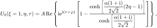 \begin{equation} U_0(\xi=1,\eta,\tau)=A \, \textrm{Re}\left\{\mathrm{i} \mathrm{e}^{\mathrm{i} (\tau+\varphi)} \left[1-\frac{\cosh\left[\dfrac{\alpha (1+\mathrm{i})}{2\sqrt{2}}(2\eta-1)\right]}{\cosh\left[\dfrac{\alpha (1+\mathrm{i})}{2\sqrt{2}}\right]}\right] \right\} , \end{equation}
where the boundary value of the pressure gradient
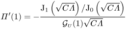 \begin{equation} \varPi'(1)={-}\frac{\textrm{J}_1\left(\sqrt{C \varLambda}\right)/\textrm{J}_0\left(\sqrt{C \varLambda}\right)}{\mathcal{G}_{\scriptscriptstyle U}(1) \sqrt{C \varLambda}} \end{equation}
has been written in terms of its modulus  $A=|\varPi '(1)|$ and argument $\varphi =\textrm {arg}[\varPi '(1)]$. Equation (4.19) will be needed in computing the flow in the edge region (see § 6.1). The order-unity factor $A$ is a measure of the stroke volume driven by the moving disk, as can be seen by writing, for example, $\int _{{\rm \pi} }^{2{\rm \pi} } [\int _{0}^1 U_0(\xi =1,\eta,\tau ) 2{\rm \pi} \, \textrm {d}\eta ] \,\textrm {d}\tau = 4{\rm \pi} A \,\textrm {Re} [ \mathrm {e}^{\mathrm {i}\varphi } \mathcal{G}_{\scriptscriptstyle {U}}(1) ]$. Its value will enter in the determination of the time-averaged levitation force (see §§ 5.2 and 6.3). The dependence of $A=|\varPi '(1)|$ on $\alpha$ and $\varLambda$, evaluated with use of (4.20) and displayed in figure 2(a), will be discussed later.
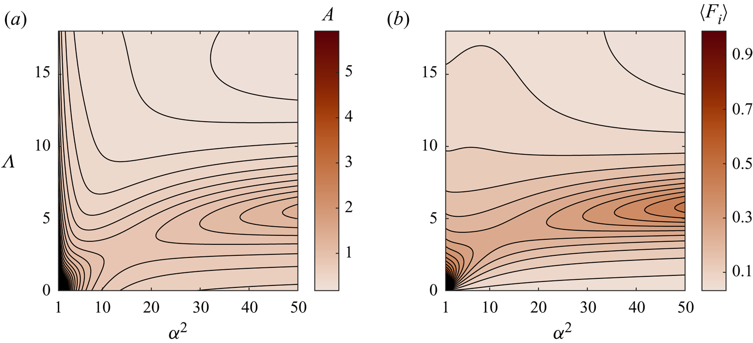
Figure 2. Variation with  $\alpha ^2$ and $\varLambda$ of (a) the stroke volume $A=|\varPi '(1)|$ evaluated with use of (4.20) and (b) the inner contribution to the levitation force $\langle F_i\rangle$ evaluated from (5.14). Computations are carried out using $\nu =0.77$, ${\textit {Pr}}=0.7$ and $\gamma =1.4$.
5. First-order correction for the pressure in the gas film
5.1. Time-averaged pressure distribution
Since the solution (4.11) is harmonic, the time-averaged values of all flow variables are identically zero (i.e.  $\langle U_0 \rangle =0$, $\langle P_0 \rangle =0, \dots$), so that the pressure at leading order does not contribute to the steady levitation force $\langle F_l \rangle$ exerted on the disk. As a result, the computation of $\langle F_l \rangle$ from (3.8) requires consideration of the time-averaged first-order correction $\langle P_1 \rangle (\xi )$ for the pressure, which yields
 \begin{equation} \langle F_l\rangle = 2 \int_0^1 \langle P_1 \rangle \xi \,\textrm{d} \xi ,\end{equation}
with small relative errors of order  $\varepsilon \sim \delta$. To determine the pressure distribution $\langle P_1 \rangle (\xi )$, one may begin by noting that the associated time-averaged radial-velocity correction $\langle U_1 \rangle$ must satisfy
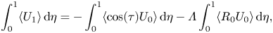 \begin{equation} \int_0^1 \langle U_1 \rangle \,\textrm{d}\eta={-}\int_0^1 \langle \cos(\tau) U_0 \rangle \,\textrm{d}\eta-\varLambda \int_0^1 \langle R_0 U_0 \rangle \,\textrm{d}\eta, \end{equation}
obtained at order  $\varepsilon$ from (3.10). Time averaging the equation that results from collecting terms of order $\varepsilon$ in the momentum equation (3.3) provides
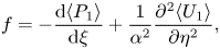 \begin{equation} f={-}\frac{\textrm{d} \langle P_1 \rangle}{\textrm{d} \xi}+\frac{1}{\alpha^2} \frac{\partial^2 \langle U_1 \rangle}{\partial \eta^2} , \end{equation}
where the known function
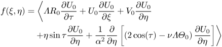 \begin{align} f(\xi,\eta) &= \left\langle\varLambda R_0{\frac{\partial U_0}{\partial \tau}} + U_0{\frac{\partial U_0}{\partial \xi}} + V_0{\frac{\partial U_0}{\partial \eta}}\right. \nonumber\\ &\quad \left. +\eta\sin\tau{\frac{\partial U_0}{\partial \eta}} + \frac{1}{\alpha^2} {\frac{\partial }{\partial \eta}}\left[ \left(2\cos(\tau)-\nu\varLambda\varTheta_0\right) {\frac{\partial U_0}{\partial \eta}} \right] \right\rangle \end{align}
can be compactly re-expressed by adding to it the time average of the left-hand side of the order-unity continuity equation (4.3), which gives
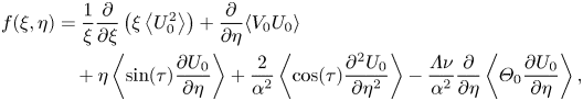 \begin{align} f(\xi,\eta)&=\frac{1}{\xi} \frac{\partial}{\partial \xi}\left(\xi \left\langle U_0^2 \right\rangle \right)+ \frac{\partial}{\partial \eta}\langle V_0 U_0 \rangle \nonumber\\ &\quad +\eta \left\langle \sin(\tau) \frac{\partial U_0}{\partial \eta} \right\rangle+\frac{2}{\alpha^2} \left\langle \cos (\tau)\frac{\partial^2 U_0}{\partial \eta^2}\right\rangle-\frac{\varLambda \nu}{\alpha^2} \frac{\partial}{\partial \eta} \left\langle \varTheta_0 \frac{\partial U_0}{\partial \eta} \right\rangle , \end{align}
both of which can be evaluated in terms of the expressions given in (4.11). Note that the terms in the expressions for  $f$ that involve $\cos (\tau )$ and $\sin (\tau )$ stem from the change of variables described in (4.2a,b). Integrating the reduced momentum equation (5.3) with the no-slip conditions $\langle U_1 \rangle =0$ at $\eta =0,1$ gives
 \begin{equation} \frac{\langle U_1 \rangle}{\alpha^2}={-}\frac{\textrm{d} \langle P_1 \rangle}{\textrm{d} \xi}\frac{(1-\eta)\eta}{2}+\eta \int_0^\eta f \,\textrm{d}\tilde{\eta}-\int_0^\eta f \tilde{\eta} \,\textrm{d}\tilde{\eta}-\eta \int_0^1 f (1-\tilde{\eta}) \,\textrm{d} \tilde{\eta}, \end{equation}
where  $\tilde {\eta }$ is a dummy integration variable. The associated radial flux,
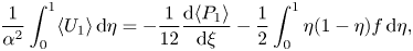 \begin{equation} \frac{1}{\alpha^2} \int_0^1 \langle U_1 \rangle \,\textrm{d} \eta={-}\frac{1}{12} \frac{\textrm{d} \langle P_1 \rangle}{\textrm{d} \xi}-\frac{1}{2} \int_0^1 \eta (1-\eta) f \,\textrm{d} \eta, \end{equation}
can be substituted into (5.2) to give
 \begin{equation} \langle P_1 \rangle' =\frac{12}{\alpha^2}\left[\int_0^1 \langle \cos(\tau) U_0 \rangle \,\textrm{d}\eta+\varLambda \int_0^1 \langle R_0 U_0 \rangle \,\textrm{d}\eta \right]-6 \int_0^1 \eta (1-\eta) f\, \textrm{d} \eta \end{equation}
for the derivative of the time-averaged pressure  $\langle P_1 \rangle '=\textrm {d} \langle P_1 \rangle /\textrm {d} \xi$. The above equation can be readily integrated to give
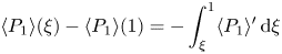 \begin{equation} \langle P_1\rangle (\xi)-\langle P_1\rangle (1)={-}\int^1_{\xi} \langle P_1 \rangle' \, \textrm{d}\xi \end{equation}
for the pressure variation from the unknown boundary value  $\langle P_1 \rangle (1)$. The above integral can be evaluated with use of (5.8) along with the identity $\langle \textrm {Re}(\mathrm {e}^{\mathrm {i} \tau } \mathcal{A} ) \textrm {Re}(\mathrm {e}^{\mathrm {i} \tau } \mathcal{B} )\rangle =\textrm {Re}(\mathcal{A} \mathcal{B}^*)/2$, which applies to any generic time-independent complex functions $\mathcal{A}$ and $\mathcal{B}$, with the asterisk $*$ denoting complex conjugates. The resulting expression can be cast in the form
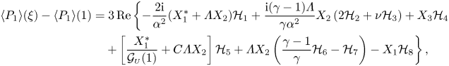 \begin{align} \langle P_1\rangle (\xi)-\langle P_1\rangle (1)&= 3\, \textrm{Re} \left\{ - \frac{2\mathrm{i}}{\alpha^2}(X^*_1 + \varLambda X_2) \mathcal{H}_1 + \frac{\mathrm{i}(\gamma-1)\varLambda}{\gamma\alpha^2} X_2 \left( 2\mathcal{H}_2 + \nu \mathcal{H}_3 \right) + X_3 \mathcal{H}_4 \right.\nonumber\\ &\quad\left. + \left[ \frac{X^*_1}{\mathcal{G}_{\scriptscriptstyle{U}}(1)} + C\varLambda X_2\right] \mathcal{H}_5 + \varLambda X_2 \left( \frac{\gamma-1}{\gamma} \mathcal{H}_6 - \mathcal{H}_7 \right) - X_1 \mathcal{H}_8 \right\} , \end{align}
which involves the complex functions  $X_i(\xi )$ and the complex constants $\mathcal{H}_j$ (with $i=1 - 3$ and $j=1 - 8$), whose expressions as functions of $\varLambda$ and $\alpha ^2$ are given in Appendix A.
5.2. An expression for the squeeze-film force
Substitution of (5.9) into (5.1) yields
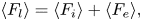 \begin{equation} \langle F_l\rangle = \langle F_i\rangle + \langle F_e\rangle , \end{equation}
where
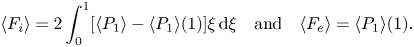 \begin{equation} \langle F_i\rangle =2 \int_0^1[\langle P_1 \rangle-\langle P_1 \rangle(1)] \xi\,\textrm{d}\xi \quad \textrm{and} \quad \langle F_e\rangle=\langle P_1\rangle (1) . \end{equation}
The first term on the right-hand side of (5.11), to be evaluated with use of
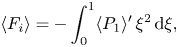 \begin{equation} \langle F_i\rangle={-}\int^1_0 \langle P_1 \rangle' \, \xi^2 \, \textrm{d} \xi, \end{equation}
obtained by integration by parts, is associated with the pressure increase in the gas film from its value at the disk edge. The integral in (5.13) can be expressed in the form
 \begin{align} \langle F_i\rangle &= 3\, \textrm{Re} \left\{ - \frac{2\mathrm{i}}{\alpha^2}(\mathcal{X}^*_1 + \varLambda \mathcal{X}_2) \mathcal{H}_1 + \frac{\mathrm{i}(\gamma-1)\varLambda}{\gamma\alpha^2} \mathcal{X}_2 \left( 2\mathcal{H}_2 + \nu \mathcal{H}_3 \right) + \mathcal{X}_3 \mathcal{H}_4 \right.\nonumber\\ &\left. \quad + \left[ \frac{\mathcal{X}^*_1}{\mathcal{G}_{\scriptscriptstyle{U}}(1)} + C\varLambda\mathcal{X}_2\right] \mathcal{H}_5 + \varLambda\mathcal{X}_2 \left( \frac{\gamma-1}{\gamma} \mathcal{H}_6 - \mathcal{H}_7 \right) - \mathcal{X}_1 \mathcal{H}_8 \right\} , \end{align}
where the complex constants  $\mathcal {X}_i=2\int _0^1 X_i \, \xi \,\textrm {d} \xi$ (with $i=1 - 3$) are given in Appendix A. The associated variation of $\langle F_i\rangle$ with $\varLambda$ and $\alpha ^2$ is depicted in figure 2(b). Limiting expressions for $\langle F_i\rangle$ are to be derived below for $\varLambda \ll 1$, $\alpha ^2 \ll 1$ and $\alpha ^2 \gg 1$.
The second term  $\langle F_e\rangle$ in (5.11), comparable in magnitude to $\langle F_i\rangle$, arises from the departure of the time-averaged pressure at the disk edge from its ambient value in the surrounding stagnant gas. The computation of this quantity requires consideration of the flow in the non-slender near-edge region, a problem to be addressed in § 6.
5.3. Limiting cases of interest
The spatial pressure variation  $\langle P_1\rangle (\xi )-\langle P_1\rangle (1)$ and its contribution $\langle F_i\rangle$ to the levitation force, given respectively in (5.10) and (5.14), admit simplified forms for limiting values of the two controlling parameters $\varLambda$ and $\alpha ^2$, to be investigated below. Consistency between each limiting solution and the respective original expression was confirmed computationally.
5.3.1. The incompressible limit  $\varLambda \ll 1$

In the limit  $\varLambda \ll 1$, the gas behaves effectively as incompressible, in that the motion is independent of the density variations, with the leading-order pressure and velocity distributions reducing to
 \begin{equation} P_0=\frac{1-\xi^2}{4} \textrm{Re} \left[ \frac{\mathrm{e}^{\mathrm{i}\tau}}{\mathcal{G}_{\scriptscriptstyle{U}}(1)} \right], \quad U_0={-}\frac{\xi}{2} \textrm{Re}\left[\mathrm{i} \mathrm{e}^{\mathrm{i} \tau} \frac{\mathcal{G}'_{\scriptscriptstyle U}(\eta)}{\mathcal{G}_{\scriptscriptstyle U}(1)} \right], \quad V_0=\textrm{Re}\left[\mathrm{i} \mathrm{e}^{\mathrm{i} \tau} \frac{\mathcal{G}_{\scriptscriptstyle U}(\eta)}{\mathcal{G}_{\scriptscriptstyle U}(1)} \right], \end{equation}
as follows from (4.11), whence the dimensionless stroke volume simplifies to
 \begin{equation} A = \frac{1}{2} \left| \frac{\beta_{\scriptscriptstyle{U}}}{\beta_{\scriptscriptstyle{U}}-\tanh\beta_{\scriptscriptstyle{U}}} \right| . \end{equation}
Using these expressions in (5.8) yields the parabolic steady overpressure distribution,
 \begin{equation} \langle P_1 \rangle (\xi) - \langle P_1 \rangle (1) = \frac{3}{8} \left(\xi^2-1\right) \textrm{Re} \left[ \frac{|\mathcal{G}_{\scriptscriptstyle{U}}'|^2-2 \mathcal{G}_{\scriptscriptstyle{U}}{\mathcal{G}_{\scriptscriptstyle{U}}^*}''}{|\mathcal{G}_{\scriptscriptstyle{U}}(1)|^2} + \frac{2 \eta \mathcal{G}_{\scriptscriptstyle{U}}''-4(1-\mathcal{G}_{\scriptscriptstyle{U}}')}{\mathcal{G}_{\scriptscriptstyle{U}}(1)}\right] , \end{equation}
substitution of which in (5.12a,b) gives
 \begin{align} \langle F_i\rangle&= \textrm{Re} \left\{ \left[ 30\beta_{\scriptscriptstyle{U}}\tanh\beta_{\scriptscriptstyle{U}}\tan\beta_{\scriptscriptstyle{U}} - (24\beta_{\scriptscriptstyle{U}}^2+3)\tanh\beta_{\scriptscriptstyle{U}} \right.\right.\nonumber\\ &\quad \left.\left.\left.+ (24\beta_{\scriptscriptstyle{U}}^2-105)\tan\beta_{\scriptscriptstyle{U}} + 4\beta_{\scriptscriptstyle{U}}^3\right] \right/ \left[128 \beta_{\scriptscriptstyle{U}}(\beta_{\scriptscriptstyle{U}}-\tanh\beta_{\scriptscriptstyle{U}})(\beta_{\scriptscriptstyle{U}}-\tan\beta_{\scriptscriptstyle{U}}) \right] \right\}, \end{align}
which is found to depend purely on the Stokes number through  $\beta _{\scriptscriptstyle {U}} = \alpha (1+\mathrm {i})/\sqrt {8}$.
5.3.2. The lubrication limit $\alpha ^2 \ll 1$

When the Stokes number assumes small values  $\alpha ^2 \ll 1$, fluid acceleration driven by disk oscillations becomes negligibly small relative to viscous diffusion of momentum. To preserve non-trivial dominant balances in the momentum (3.3) and state (3.5) equations with $\alpha ^2\to 0$, the dimensionless pressure, temperature and density variables must be rescaled appropriately as
 \begin{equation} \frac{\bar{P}}{\alpha^2 P}=\frac{\bar{R}}{\alpha^2 R} = \frac{\bar{\varTheta}}{\alpha^2 \varTheta}=1 , \end{equation}
substitution of which into the energy equation (3.4) gives  $\partial ^2\bar {\varTheta }/\partial Y^2=0$ for $\alpha ^2\to 0$, whence $\bar {\varTheta }=0$ owing to the isothermal conditions on the bounding surfaces. It follows then from the state equation that $\bar {P}=\bar {R}$, and from the reduced momentum equation $\partial \bar {P}/\partial \xi = \partial ^2U/\partial Y^{2}$ that the radial velocity component varies across the gas layer in terms of the classical Poiseuille profile
 \begin{equation} U(\xi,Y,\tau) ={-} \frac{\partial \bar{P}}{\partial \xi} \frac{(H-Y)Y}{2} , \end{equation}
consistent with the non-slip conditions on the walls. Integrating the continuity equation (3.2) across the gas film using the known expressions for  $\bar {R}$ and $U$ yields
 \begin{equation} \sigma\frac{\partial (H\bar{P})}{\partial \tau} - \frac{H^3}{\xi}\frac{\partial}{\partial \xi} \left[ \left( 1+\varepsilon\frac{\sigma}{12}\bar{P} \right) \xi \frac{\partial \bar{P}}{\partial \xi} \right] - 12\sin\tau = 0 , \end{equation}
the relevant isothermal squeeze-film equation, whence the radial pressure distribution can be determined solely in terms of
 \begin{equation} \sigma = \frac{12\varLambda}{\alpha^2}=\frac{12\mu_a\omega a^2}{p_a h_o^2} , \end{equation}
a similarity parameter unique to the lubrication limit known as the squeeze number (see Langlois Reference Langlois1962). Solving (5.21) using the truncated expansion  $\bar {P}=\bar {P}_0+\varepsilon \bar {P}_1$ yields
 \begin{equation} \alpha^2 A = 12\left| \frac{ \textrm{J}_1\left(\beta_{\sigma}\right)}{ \beta_{\sigma} \textrm{J}_0\left(\beta_{\sigma}\right) } \right| , \quad\textrm{where}\ \beta_{\sigma} = \sqrt{\sigma}\,\frac{(1+\mathrm{i})}{\sqrt 2} , \end{equation}
for the characteristic value of the stroke volume and
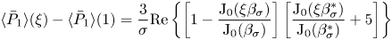 \begin{equation} \langle \bar{P}_1 \rangle (\xi) - \langle \bar{P}_1 \rangle (1) = \frac{3}{\sigma} \textrm{Re} \left\{ \left[ 1 - \frac{\textrm{J}_0(\xi\beta_{\sigma})}{\textrm{J}_0(\beta_{\sigma})} \right] \left[ \frac{\textrm{J}_0(\xi\beta_{\sigma}^*)}{\textrm{J}_0(\beta_{\sigma}^*)} +5 \right] \right\} \end{equation}
for the time-averaged pressure distribution, the latter providing
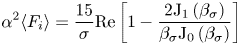 \begin{equation} \alpha^2\langle F_i\rangle= \frac{15}{\sigma} \textrm{Re} \left[ 1 - \frac{2\textrm{J}_1\left(\beta_{\sigma}\right) }{ \beta_{\sigma} \textrm{J}_0\left(\beta_{\sigma}\right)} \right] \end{equation}
for the corresponding contribution to the levitation force. Since, as shall be proven in § 6.4, the edge pressure  $\langle \bar {P}_1\rangle (1)$ is identically zero when $\alpha ^2=0$, (5.24) recovers exactly the results found by Taylor & Saffman (Reference Taylor and Saffman1957). Expressions for the large values of $A$ and $\langle F_i\rangle$ found near the origin of the $\varLambda -\alpha ^2$ diagrams of figure 2 follow from taking the limit $\sigma \ll 1$ in (5.23) and (5.25) to give
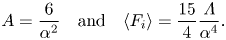 \begin{equation} A=\frac{6}{\alpha^2} \quad \textrm{and} \quad \langle F_i\rangle=\frac{15}{4} \frac{\varLambda}{\alpha^4}. \end{equation}
5.3.3. The inviscid limit $\alpha ^2 \gg 1$

When  $\alpha ^2 \to \infty$, viscous diffusion, significantly outpaced by fluid acceleration, is confined to vanishingly thin near-wall boundary layers. Note that under the limit of slender flow $h_o/a\ll 1$, the interference of transverse acoustic waves in the gas film can be neglected because the acoustic wavenumber $K = \sqrt {\varLambda /\gamma }\sim 1$ is of order-unity. Upon relaxation of the non-slip boundary conditions, the leading-order solution reduces to
 \begin{equation} P_0 = \varPi\cos(\tau) , \quad U_0 ={-}\varPi'\sin(\tau) , \quad V_0 ={-}\eta\sin(\tau) , \end{equation}
where the reduced pressure  $\varPi$ and its gradient $\varPi '$ have simplified to
 \begin{equation} \varPi(\xi) = \frac{ \left.\textrm{J}_0\left(K \xi \right) \right/ \textrm{J}_0\left(K\right) - 1}{K^2} \quad \textrm{and} \quad \varPi'(\xi) ={-} \frac{ \left.\textrm{J}_1\left(K \xi\right) \right/ \textrm{J}_0\left(K\right)}{K} , \end{equation}
which yields
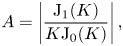 $$\begin{gather} A=\left|\frac{\textrm{J}_1(K)}{K \textrm{J}_0(K)} \right|, \end{gather}$$
 $$\begin{gather}\langle P_1 \rangle (\xi) - \langle P_1 \rangle (1) = \frac{ \textrm{J}_1^2(K) - \textrm{J}_1^2(K\xi) + \left[ \textrm{J}_0^2(K) - \textrm{J}_0^2(K\xi) \right]^2}{ 4K^2 \textrm{J}_0^2(K) } \end{gather}$$
and
 \begin{equation} \langle F_i\rangle=\frac{1}{4K^2} \left[ 1 +\frac{\textrm{J}_1\left(K\right)}{\textrm{J}_0\left(K\right)} \left(\frac{\textrm{J}_1\left(K\right)}{\textrm{J}_0\left(K\right)} - \frac{2}{K} \right) \right] , \end{equation}
all of which depend solely on  $\varLambda$ through the acoustic wavenumber $K= \sqrt {\varLambda /\gamma }$. Note that in the inviscid limit, the predicted values of $A$ and $\langle F_i\rangle$ become unbounded when $K = \sqrt {\varLambda /\gamma }=2.4048,5.5201,\dots$ corresponding to the zeros of the Bessel function $\textrm {J}_0$. For example, for the value $\gamma =1.4$ used in generating the results of figure 2, the first singularity develops at $\varLambda =8.096$ as $\alpha \rightarrow \infty$ from the local maxima of $A$ and $\langle F_i\rangle$ observed near $\varLambda \simeq 6$ for $\alpha ^2=50$.
6. Leading-order solution in the edge region
6.1. Problem formulation
As previously discussed, the non-slender flow at distances of order  $h_o$ from the disk edge involves velocities of order $u \sim v \sim u_c=\varepsilon \omega a$ and spatial pressure differences of order $\delta \Delta p \sim \varepsilon \Delta p=\rho _a u_c^2$. The description below employs the local rescaled coordinates $X=(r-a)/h_o$ and $Y=y/h_o$. The velocity must match with that found at the edge of the slender gaseous film, given at leading order in (4.19). To facilitate the matching and reduce the parametric dependence of the solution, it is convenient to introduce a shifted time variable $\hat {\tau }=\tau +\varphi$ and use the local velocity $A u_c$ in the definition of the dimensionless variables $\boldsymbol {\hat {V}}=(\hat {U},\hat {V})=[u/(A u_c),v/(A u_c)]$ and $\hat {P}=(p-p_a)/(\rho _a A^2 u_c^2)$. Substitution of these definitions into the reduced local conservation equations (2.8) and (2.9) gives, with errors of order $\varepsilon \sim \delta$,
 $$\begin{gather} \boldsymbol{\nabla}\boldsymbol{\cdot} \boldsymbol{\hat{V}}=0, \end{gather}$$
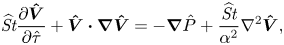 $$\begin{gather}\widehat{{\textit{St}}} \frac{\partial \boldsymbol{\hat{V}}}{\partial \hat{\tau}}+ \boldsymbol{\hat{V}} \boldsymbol{\cdot}\boldsymbol{\nabla} \boldsymbol{\hat{V}}={-}\boldsymbol{\nabla} \hat{P}+ \frac{\widehat{{\textit{St}}}}{\alpha^2} \nabla^2 \boldsymbol{\hat{V}}, \end{gather}$$
where  $\boldsymbol {\nabla }=(\partial /\partial X,\partial /\partial Y)$. As a result of the choice of velocity scale, the Strouhal number enters above in the normalized form
 \begin{equation} \widehat{{\textit{St}}}=\frac{h_o/(A u_c)}{\omega^{{-}1}}=\frac{\delta/\varepsilon}{A}. \end{equation}
This additional parameter is of order unity in the distinguished limit  $\varepsilon \sim \delta$ considered here, with $\hat {Re}=\alpha ^2/\widehat {{\textit {St}}}=\rho _a A u_c h_o/\mu _a$ being the corresponding Reynolds number.
Equations (6.1) and (6.2) must be integrated for each of the three geometric configurations of the edge region (see figure 1), with the condition that the velocity must be zero on the walls:
 \begin{equation} \hat{\boldsymbol{V}} =
0 \quad\textrm{at}\ \begin{cases} (X\leqslant0,Y=1) ;\quad
Y=0 ;\quad (X=0 , Y\geqslant1) &
\textrm{for piston--wall} \\
(X\leqslant0, Y=0,1) ;\quad (X=0, Y\leqslant0\,|\,
Y\geqslant1) & \textrm{for
piston--piston} \\ (X\leqslant0, Y=1) ;\quad Y=0
& \textrm{for disk--wall,}
\end{cases} \end{equation}
\begin{equation} \hat{\boldsymbol{V}} =
0 \quad\textrm{at}\ \begin{cases} (X\leqslant0,Y=1) ;\quad
Y=0 ;\quad (X=0 , Y\geqslant1) &
\textrm{for piston--wall} \\
(X\leqslant0, Y=0,1) ;\quad (X=0, Y\leqslant0\,|\,
Y\geqslant1) & \textrm{for
piston--piston} \\ (X\leqslant0, Y=1) ;\quad Y=0
& \textrm{for disk--wall,}
\end{cases} \end{equation}
and must vanish in the open atmosphere, where the pressure must correspondingly approach its ambient value, so that
 \begin{equation} \hat{\boldsymbol{V}} \to 0 \quad\textrm{and}\quad \hat{P} \to 0 \quad\textrm{as}\ X^2+Y^2\to\infty . \end{equation}
Matching with the velocity found at the edge of the slender gas layer, given at leading order in (4.19), provides the additional boundary condition (common to all three geometries)
 \begin{equation} \hat{U}-\textrm{Re}\left\{\mathrm{i} \mathrm{e}^{\mathrm{i} \hat{\tau}} \left[1-\frac{\cosh\left[\dfrac{\alpha (1+\mathrm{i})}{2\sqrt{2}}(2Y-1)\right]}{\cosh\left[\dfrac{\alpha (1+\mathrm{i})}{2\sqrt{2}}\right]}\right] \right\}= \hat{V}=0 \quad \textrm{as} \ X \rightarrow -\infty \quad \textrm{for} \ 0\leqslant Y \leqslant 1, \end{equation}
consistent with an accompanying pressure distribution of the form
 \begin{equation} \hat{P}=\widehat{{\textit{St}}} \cos(\hat{\tau}) X+\hat{P}_\infty(\hat{\tau}) \quad \textrm{as} \ X \rightarrow -\infty \quad \textrm{for} \ 0\leqslant Y \leqslant 1, \end{equation}
where the time-dependent pressure offset  $\hat {P}_\infty (\hat {\tau })$ exhibits a time-averaged component $\langle \hat {P}_\infty \rangle = \hat{P}_e$.
6.2. Selected numerical results
The solution in the near-edge region depends on two parameters, namely, the Strouhal number  $\widehat {{\textit {St}}}$, which measures unsteady effects in (6.2), and the Stokes number $\alpha ^2$, which measures viscous forces in (6.2) and enters also through the boundary condition (6.6). The numerical integration was based on the weak formulation of the Navier–Stokes equations (6.1) and (6.2). A Lagrange–Galerkin second-order temporal finite difference scheme using the rescaled time variable $\hat {\tau }/\widehat {{\textit {St}}}$ was employed along with P2/P1 Taylor–Hood finite elements for velocity and pressure. The resulting system of partial difference equations was implemented in the open source software FreeFEM (Hecht Reference Hecht2012) in conjunction with the MUMPS framework (Multifrontal Massively Parallel sparse direct Solver). Further details regarding the numerical method are available in an exemplary analysis by Carpio, Prieto & Vera (Reference Carpio, Prieto and Vera2016).
Three computational meshes were designed to represent the different geometrical configurations of the edge region (see figure 1), each consisting of non-slip boundaries representing the solid surfaces listed in (6.4), an inner boundary at  $-X=\ell _n\gg 1$ for $0\leqslant Y\leqslant 1$, where the matching velocity (6.6) was imposed and a circular-arc outer boundary at $(X^2+Y ^2)^{1/2}=\ell _p \gg 1$ representing the stagnant surroundings. The advective boundary condition $\widehat {{\textit {St}}}\,\partial \hat {\boldsymbol {V}}/\partial \tau + \hat {\boldsymbol {V}}\boldsymbol {\cdot }\boldsymbol {\nabla }\hat {\boldsymbol {V}}=0$ was applied along this finite ambient boundary in place of the original condition (6.5) to assist numerical convergence. To ease constraints on spatial discretization, the disk in the disk–wall configuration was given a finite relative thickness of $0.1$. Each triangulated grid was refined near the mouth of the gas film $X=0$ to allow better characterization of the anticipated shedding of vorticity into the surroundings. Convergence tests were conducted to verify the validity of each mesh with regards to the choice of dimensions $\ell _n$ and $\ell _p$ and of spatial and temporal resolution.
Each computation was initialized with stagnant conditions ( $\hat {\boldsymbol {V}}=0,\hat {P}=0$) and carried out until a $2{\rm \pi}$ periodic solution was reached, the criterion for convergence being that the relative difference between the computed values of the constant $\hat{P_e}$ be less than or approximately $0.5\,\%$ over subsequent cycles. While the number of cycles necessary for convergence was found to vary weakly with the two governing parameters, the time step required for stability became restrictively small for large values of the Reynolds number $\hat {Re}=O(100)$.
Illustrative results obtained for  $\alpha ^2=20$ and $\widehat {{\textit {St}}}=0.5$ for the three geometrical configurations (piston–wall, piston–piston and disk–wall) are shown in figure 3. The plots represent distributions of flow speed and associated instantaneous streamlines at selected instants of time $\hat {\tau }$ differing by a semi-period of the driving oscillations (6.6). The results shown in panels (a–c) are for $\hat {\tau }=2 n{\rm \pi} -{\rm \pi} /2$, corresponding to outflow, while those in panels (d–f) are for $\hat {\tau }=2 n{\rm \pi} +{\rm \pi} /2$, corresponding to inflow (where $n$ is any positive natural number).
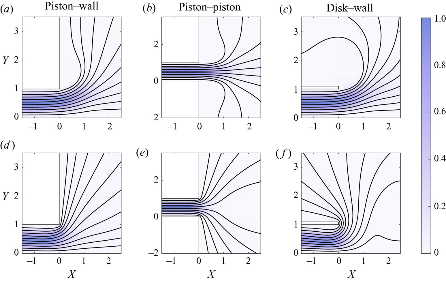
Figure 3. Streamlines for  $\alpha ^2=20, \widehat {{\textit {St}}}=0.5 \ (\hat {Re}=40)$ in the edge flow regions of the three geometric configurations presented in figure 1, shaded to represent the flow speed $(\hat {U}^2+\hat {V}^2)^{1/2}$. The images of outflow along the top row (a–c) correspond to values of time $\hat {\tau }=2 n{\rm \pi} -{\rm \pi} /2$ and those representing inflow (d–f) correspond to $\hat {\tau }=2 n{\rm \pi} +{\rm \pi} /2$, where $n\in \mathbb {N}$.
Although the driving velocity (6.6) is time-harmonic, the nonlinearity induced by convective acceleration in (6.2) yields non-harmonic velocities  $\hat {\boldsymbol {V}}$ and pressures $\hat {P}$ in the region of fluid exchange between the gaseous film and the stagnant surroundings. This non-harmonic periodicity, clearly noticeable for the Reynolds number $\hat {Re}=40\gg 1$ represented in figure 3, is evidenced by the asymmetry between the streamlines depicting outflow (3a–c) and those depicting inflow (3d–f), associated with non-zero values of the resulting time-averaged velocity $\langle \hat {\boldsymbol {V}}\rangle$. The degree of nonlinearity can also be anticipated to hold strong correlation with the magnitude of the time-averaged pressure $\langle \hat {P}\rangle$, which approaches the asymptotic value $\langle \hat {P}\rangle =\hat {P}_e$ in the gas film as $X\rightarrow -\infty$, as indicated below (6.7).
6.3. Pressure drop across the edge region
The constant  $\hat {P}_e$, which represents the time-averaged pressure drop across the near-edge region, was determined as part of the numerical integration. Its value is related to the unknown boundary value $\langle P_1 \rangle (1)$ of the pressure distribution in the gaseous film, which determines the second contribution $\langle F_e\rangle =\langle P_1 \rangle (1)$ to the levitation force (5.11). Their relation can be established by noting that the variables $P$ and $\hat {P}$ satisfy $P=\varepsilon A^2 \hat {P}$, as follows from their respective definitions. Substituting the two-term expansion $P=P_0+\varepsilon P_1$ and using the limiting pressure distribution (6.7) reveals that matching the pressure fields in the slender film and in the near-edge region requires that $P_0=0$ at $\xi =1$, which is the boundary condition imposed for the inner problem at leading order in (4.8), and additionally that
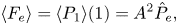 \begin{equation} \langle F_e\rangle=\langle P_1 \rangle(1)=A^2 \hat{P}_e, \end{equation}
where  $A=|\varPi '(1)|(\varLambda,\alpha ^2)$ is the dimensionless stroke volume represented in figure 2(a). The computation of $\hat {P}_e$ is therefore essential to enable the evaluation of the force experienced by the disk. It is worth noting that the expression for the steady squeeze-film force (5.11), originating from (2.7), does not account for the variations of $\langle \hat {P} \rangle$ from $\hat {P}_e$ that occur in the edge region at distances $-X \sim 1$. This higher-order effect, not considered here, could be incorporated into the analysis, providing a small relative correction, of order $\delta \sim \varepsilon$, to the force experienced by the disk.
The variation of  $\hat {P}_e$ with $\alpha ^2$ corresponding to the piston–wall geometry is represented in figure 4(a) for selected values of $\widehat {{\textit {St}}}$. As can be seen, $\hat {P}_e$ is always negative, which indicates that the time-averaged pressure near the entrance of the gas film is always smaller than the ambient value, with the magnitude of the pressure drop becoming larger for larger values of $\widehat {{\textit {St}}}$. As demonstrated by the results shown in figure 4(b) for $\widehat {{\textit {St}}}=5$, the dependence of $\hat {P}_e$ on the geometrical configuration is fairly weak, well in qualitative accordance with the experimental observations of Hong et al. (Reference Hong, Zhai, Yan and Wei2014). The curves corresponding to the piston–piston and piston–wall configurations are nearly indistinguishable, while that for the disk–wall geometry exhibits departures of little over $5\,\%$ from the other two curves. It is worth noting that the dependences of $\hat {P_e}$ on $\widehat {{\textit {St}}}$ and on the geometrical configuration entirely disappear as the Stokes number becomes small, where all solution curves adopt an identical parabolic shape. Also of interest is that, as seen in figure 4(b), the variation of $\hat{P_e}$ with $\alpha ^2$ is in general non-monotonic, with the pressure drop reaching a minimum at an intermediate value of $\alpha ^2$ before increasing to approach a finite asymptotic value as $\alpha ^2 \rightarrow \infty$. The limiting behaviours of the solution for $\alpha ^2 \ll 1$ and $\alpha ^2 \gg 1$ are to be further investigated below.
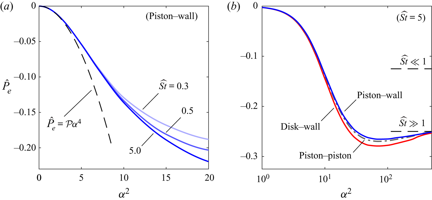
Figure 4. Variation of the steady edge pressure  $\hat {P_e}$ with $\alpha ^2$ and (a) selected values of $\widehat {{\textit {St}}}$, for the piston–wall configuration and (b) the three geometrical configurations indicated in figure 1, for $\widehat {{\textit {St}}}=5$. The dashed curve in panel (a) corresponds to the asymptotic prediction $\hat{P}_e=\mathcal{P}\alpha ^4$ corresponding to $\alpha ^2 \ll 1$, while the horizontal dashed lines in panel (b) correspond to the asymptotic predictions given in (6.23) and (6.28) for $\alpha ^2 \gg 1$ and extreme values of $\widehat {{\textit {St}}}$.
6.4. Creeping flow for $\alpha ^2 \ll 1$

Because the motion is driven by the boundary velocity profile at the edge of the gas film, the analysis of the limit  $\alpha ^2 \ll 1$ begins by expressing (6.6) in the power-series form
 \begin{equation} \hat{U}=\alpha^2 \big[\tfrac{1}{2} Y(Y-1) \cos \hat{\tau} + \alpha^2 \mathcal{S}_1(Y) \sin \hat{\tau} + \alpha^4 \mathcal{S}_2(Y) \cos \hat{\tau} +\cdots\big] , \end{equation}
where  $\mathcal{S}_1(Y), \mathcal{S}_2(Y), \ldots$ are polynomial functions of increasing degree. Since $\hat {U} \sim \alpha ^2$ while $\hat {P} \sim 1$, the latter following from the balance between viscous and pressure forces in (6.2), it appears convenient to introduce perturbation expansions of the form
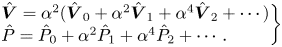 \begin{equation} \left.\begin{array}{l@{}l} {\hat{\boldsymbol{V}}}=\alpha^2 ({\hat{\boldsymbol{V}}}_0+\alpha^2 {\hat{\boldsymbol{V}}}_1+\alpha^4 {\hat{\boldsymbol{V}}}_2 +\cdots)\\ \hat{P} = \hat{P}_0+\alpha^2\hat{P}_1+\alpha^4\hat{P}_2+\cdots . \end{array}\right\} \end{equation}
Substituting the above expressions into (6.1) and (6.2) and collecting terms in powers of  $\alpha ^2$ leads to a hierarchy of problems that can be solved sequentially.
At leading order, both  $\hat {\boldsymbol {V}}_0$ and $\hat {P}_0$ are linearly proportional to $\cos \hat {\tau }$. The solution can be simplified by introduction of the time-independent reduced variables
 \begin{equation} {\tilde{\boldsymbol{V}}}_0(X,Y)= {{\hat{\boldsymbol{V}}}_0}/{\cos \hat{\tau}} \quad \textrm{and} \quad \tilde{P}_0(X,Y)=\hat{P}_0/(\widehat{{\textit{St}}} \cos \hat{\tau}), \end{equation}
which satisfy
 \begin{equation} \boldsymbol{\nabla}\boldsymbol{\cdot} {\tilde{\boldsymbol{V}}}_0=0, \quad 0={-} \boldsymbol{\nabla} \tilde{P}_0+ \nabla^2 {\tilde{\boldsymbol{V}}}_0, \end{equation}
with no-slip boundary conditions (6.4) at the walls, the stagnant-flow condition (6.5) in the ambient atmosphere and
 \begin{equation} {\tilde{\boldsymbol{V}}}_0 \rightarrow \big[\tfrac{1}{2} Y (Y-1),0\big] \quad \textrm{as} \ X \rightarrow -\infty \quad \textrm{for} \ 0\leqslant Y \leqslant 1, \end{equation}
the latter corresponding to a pressure gradient  $\partial \tilde {P}_0/\partial X=1$, consistent with the first term in (6.7). The parameter-free problem defined above, corresponding to steady Stokes flow at the mouth of a planar channel, was solved numerically to determine the function $\tilde {\boldsymbol {V}}_0(X,Y)$ for the three different geometries considered here. Note that the associated pressure $\hat {P}_0 =\widehat {{\textit {St}}} \tilde {P}_0(X,Y) \cos \hat {\tau }$ has a vanishing time-averaged value $\langle \hat {P}_0 \rangle =0$, which indicates that the pressure drop $\hat {P}_e$ is identically zero at this order.
At the following order ( $\alpha ^2$), the conservation equations are
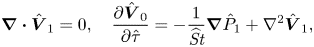 \begin{equation} \boldsymbol{\nabla}\boldsymbol{\cdot} {\hat{\boldsymbol{V}}}_1=0, \quad \frac{\partial {\hat{\boldsymbol{V}}}_0}{\partial \hat{\tau}}={-}\frac{1}{\widehat{{\textit{St}}}} \boldsymbol{\nabla} \hat{P}_1+ \nabla^2 {\hat{\boldsymbol{V}}}_1, \end{equation}
with the first-order correction for the velocity satisfying
 \begin{equation} {\hat{\boldsymbol{V}}}_1 \rightarrow [\mathcal{S}_1(Y) \sin \hat{\tau},0] \quad \textrm{as} \ X \rightarrow -\infty \quad \textrm{for} \ 0\leqslant Y \leqslant 1. \end{equation}
Inspection of the above equations reveals that  $\hat {\boldsymbol {V}}_1$ and $\hat {P}_1$ are both linearly proportional to $\sin \hat {\tau }$, so that their time-averaged values are also identically zero. Hence, the computation of the pressure drop $\hat {P}_e$ requires consideration of the problem that arises at $O(\alpha ^4)$, which comprises the conservation equations
 \begin{equation} \boldsymbol{\nabla}\boldsymbol{\cdot} {\hat{\boldsymbol{V}}}_2=0, \quad \widehat{{\textit{St}}} \frac{\partial {\hat{\boldsymbol{V}}}_1}{\partial \hat{\tau}}+{\hat{\boldsymbol{V}}}_0 \boldsymbol{\cdot} \boldsymbol{\nabla} {\hat{\boldsymbol{V}}}_0 ={-}\boldsymbol{\nabla} \hat{P}_2+ \widehat{{\textit{St}}} \nabla^2 {\hat{\boldsymbol{V}}}_2, \end{equation}
with  $\hat {\boldsymbol {V}}_2$ satisfying the matching condition
 \begin{equation} {\hat{\boldsymbol{V}}}_2 \rightarrow [\mathcal{S}_{2}(Y) \cos \hat{\tau},0] \quad \textrm{as} \ X \rightarrow -\infty \quad \textrm{for} \ 0\leqslant Y \leqslant 1. \end{equation}
Because  $\hat {\boldsymbol {V}}_0=\tilde {\boldsymbol {V}}_0(X,Y) \cos \hat {\tau }$ and $\langle \cos ^2 \hat {\tau } \rangle =1/2$, the nonlinear convective acceleration yields a non-zero contribution $\langle \hat {\boldsymbol {V}}_0 \boldsymbol {\cdot } \boldsymbol {\nabla } \hat {\boldsymbol {V}}_0\rangle = \tfrac {1}{2} \tilde {\boldsymbol {V}}_0 \boldsymbol {\cdot } \boldsymbol {\nabla } \tilde {\boldsymbol {V}}_0$ when taking the time average of the above problem, which results in a steady-streaming motion with non-zero values of $\langle \hat {\boldsymbol {V}}_2 \rangle$ and $\langle \hat {P}_2 \rangle$. To emphasize the parameter-free nature of the resulting time-averaged pressure distribution, it is of interest to incorporate the Strouhal number in the definition of the steady-streaming velocity $\hat {\boldsymbol {V}}_{\scriptscriptstyle {SS}}=\widehat {{\textit {St}}} \langle \hat {\boldsymbol {V}}_2 \rangle$, to be determined, along with the pressure $\hat {P}_{\scriptscriptstyle {SS}}= \langle \hat {P}_2 \rangle$, by integration of
 \begin{equation} \boldsymbol{\nabla} \boldsymbol{\cdot} {\hat{\boldsymbol{V}}}_{\scriptscriptstyle{SS}}=0, \quad \tfrac{1}{2} {\tilde{\boldsymbol{V}}}_0 \boldsymbol{\cdot} \boldsymbol{\nabla} {\tilde{\boldsymbol{V}}}_0 ={-}\boldsymbol{\nabla} \hat{P}_{\scriptscriptstyle{SS}}+ \nabla^2 {\hat{\boldsymbol{V}}}_{\scriptscriptstyle{SS}}, \end{equation}
with boundary conditions  $\hat {\boldsymbol {V}}_{\scriptscriptstyle {SS}}=0$ at the solid boundaries, $\hat {\boldsymbol {V}}_{\scriptscriptstyle {SS}} = \hat {P}_{\scriptscriptstyle {SS}} = 0$ in the surrounding atmosphere and
 \begin{equation} {\hat{\boldsymbol{V}}}_{\scriptscriptstyle{SS}} \rightarrow 0 \quad \textrm{as} \ X \rightarrow -\infty \quad \textrm{for} \ 0\leqslant Y \leqslant 1. \end{equation}
 Numerical integration of the above hierarchy of problems, with use of an advective condition at the finite outer boundary analogous to that described in § 6.2, determines, in particular, the (negative) value  $\mathcal{P}$ of $\hat {P}_{\scriptscriptstyle {SS}}$ as $X \rightarrow -\infty$ for $0\leqslant Y \leqslant 1$, which yields
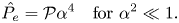 \begin{equation} \hat{P_e}=\mathcal{P}\alpha^4 \quad \textrm{for} \ \alpha^2 \ll 1. \end{equation}
With  $\tilde {\boldsymbol {V}}_0$ being also independent of $\widehat {{\textit {St}}}$, the solution depends only on the geometrical configuration. The resulting values of $\mathcal{P}$ were found to be effectively identical for all three configurations (i.e. $\mathcal{P}=-(2.67803,2.67815,2.67714)\times 10^{-3}$ for the piston–wall, piston–piston and disk–wall configurations, respectively), which indicates that for $\alpha ^2 \ll 1$, the pressure drop across the edge region is fundamentally related to the flow between the two parallel surfaces, while the flow outside exerts a lesser influence. To illustrate the accuracy of the asymptotic results for $\alpha ^2 \ll 1$, the parabolic prediction (6.20) is compared in figure 4(a) with the results of the numerical integrations of the complete Navier–Stokes equations (6.1) and (6.2).
6.5. Inviscid flow for $\alpha ^2 \gg 1$

In the limit of large Stokes numbers, the conservation equations describing edge flow (6.1) and (6.2) reduce to the Euler equations
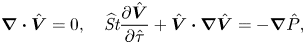 \begin{equation} \boldsymbol{\nabla} \boldsymbol{\cdot} \hat{\boldsymbol{V}}=0, \quad \widehat{{\textit{St}}} \frac{\partial \hat{\boldsymbol{V}}}{\partial \hat{\tau}}+\hat{\boldsymbol{V}} \boldsymbol{\cdot} \boldsymbol{\nabla} \hat{\boldsymbol{V}} ={-}\boldsymbol{\nabla} \hat{P}, \end{equation}
subject to the condition of no penetration along the solid boundaries and the oscillating plug-flow velocity
 \begin{equation} \hat{\boldsymbol{V}} \rightarrow [-\sin\hat{\tau},0] \quad \textrm{as} \ X \rightarrow -\infty \quad \textrm{for} \ 0\leqslant Y \leqslant 1, \end{equation}
the latter following from (6.6) when  $\alpha ^2 \gg 1$. Vorticity is confined to thin layers of relative thickness $\alpha ^{-1}$, which include near-wall boundary layers and a vortex sheet of evolving shape (two for the piston–piston geometry) originating at the rim(s) of the disk/piston(s). In this limit $\alpha ^2 \gg 1$, numerical integration of the associated time-dependent free-boundary problem, needed to determine the nearly inviscid value $\hat {P}_i(\widehat {{\textit {St}}})$ of $\hat {P_e}$, is a difficult task, not to be pursued below. Instead, we shall focus on the solutions arising in the two limiting cases $\widehat {{\textit {St}}}\ll 1$ and $\widehat {{\textit {St}}}\gg 1$, which are amenable to an analytical description.
In the quasi-steady limit  $\widehat {{\textit {St}}} \ll 1$, the local acceleration term in (6.21a,b) can be neglected in the first approximation, so that the familiar Bernoulli's equation $\hat {P}+|\hat {\boldsymbol {V}}|^2/2=\textrm {const}.$ applies along streamlines. The solution that emerges can be anticipated to be drastically different for inflow (i.e. $0<\hat {\tau }< {\rm \pi}$) and outflow (i.e. ${\rm \pi} < \hat {\tau }< 2{\rm \pi}$). During the outflow semi-cycle, the stream along the gas film separates at the exit section to form a planar jet that discharges with parallel streamlines surrounded by nearly stagnant ambient fluid. In that case, the pressure along the film remains equal to the ambient pressure $\hat {P}=0$. For inflow, however, the ambient gas accelerates from rest along streamlines approaching the canal entrance from all directions. Conservation of total head $\hat {P}+|\hat {\boldsymbol {V}}|^2/2=0$ yields $\hat {P}=-\sin ^2(\hat {\tau })/2$ for the pressure along the film away from the entrance. Consequently, because $\hat {P}=0$ in the gas film during outflow (i.e. for ${\rm \pi} \leqslant \hat {\tau } \leqslant 2 {\rm \pi}$), the time-averaged pressure drop, obtained by taking the time average of the gas-film pressure over a period, reduces to
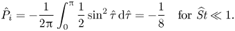 \begin{equation} \hat{P}_i={-}\frac{1}{2{\rm \pi}} \int_0^{\rm \pi} \frac{1}{2} \sin^2 \hat{\tau} \, \textrm{d}\hat{\tau}={-}\frac{1}{8} \quad \textrm{for} \ \widehat{{\textit{St}}} \ll 1. \end{equation}
 In the nearly acoustic limit of large Strouhal numbers  $\widehat {{\textit {St}}}\gg 1$, it is convenient to introduce perturbation expansions in integral powers of the inverse of the Strouhal number
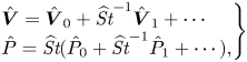 \begin{equation} \left. \begin{array}{l@{}l} \hat{\boldsymbol{V}} = \hat{\boldsymbol{V}}_0 + \widehat{{\textit{St}}}^{{-}1}\hat{\boldsymbol{V}}_1 + \cdots\\ \hat{P} = \widehat{{\textit{St}}}(\hat{P}_0 + \widehat{{\textit{St}}}^{{-}1} \hat{P}_1 + \cdots) , \end{array}\right\} \end{equation}
based on the anticipated scales of pressure and velocity. At leading order, we find the linear equations
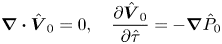 \begin{equation} \boldsymbol{\nabla}\boldsymbol{\cdot} \hat{\boldsymbol{V}}_0=0, \quad \frac{\partial \hat{\boldsymbol{V}}_0}{\partial \hat{\tau}} ={-}\boldsymbol{\nabla} \hat{P}_0 \end{equation}
to be integrated with the boundary condition
 \begin{equation} \hat{\boldsymbol{V}}_0 \rightarrow [-\sin\hat{\tau},0] \quad \textrm{as} \ X \rightarrow -\infty \quad \textrm{for} \ 0\leqslant Y \leqslant 1. \end{equation}
The velocity field is potential and can be correspondingly determined for each geometrical configuration with use of conformal mapping techniques (Birkhoff & Zarantonello Reference Birkhoff and Zarantonello1957; Gurevich Reference Gurevich1966). Note that since  $\hat {P}_0 \propto \cos \hat {\tau }$, the time-averaged pressure is identically zero at this order. The value of $\hat {P}_i$ can be obtained by taking the time average of the momentum equation that emerges at the following order,
 \begin{equation} \frac{\partial \hat{\boldsymbol{V}}_1}{\partial \hat{\tau}}+\boldsymbol{\nabla} \left( \hat{P}_1 + \frac{|\hat{\boldsymbol{V}}_0|^2}{2} \right) = 0, \end{equation}
which yields  $\langle \hat {P}_1 \rangle +\langle |\hat {\boldsymbol {V}}_0|^2\rangle /2=\textrm {const}.$, which can be evaluated in the ambient gas to give $\langle \hat {P}_1 \rangle =-\langle |\hat {\boldsymbol {V}}_0|^2\rangle /2$ for the spatial distribution of time-averaged pressure. Upon evaluating $\langle \hat {P}_1 \rangle$ inside the slender film with use of (6.26), we finally obtain the limiting value
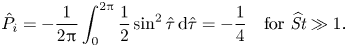 \begin{equation} \hat{P}_i={-}\frac{1}{2{\rm \pi}} \int_0^{2{\rm \pi}} \frac{1}{2} \sin^2 \hat{\tau} \, \textrm{d}\hat{\tau}={-}\frac{1}{4} \quad \textrm{for} \ \widehat{{\textit{St}}} \gg 1. \end{equation}
 The asymptotic values (6.23) and (6.28) serve as bounds of the large– $\alpha ^2$ asymptotic behaviour of $\hat {P_e}$. Both values are indicated using dashed lines in figure 4(b). It should be noted that these bounds do not apply for finite values of the Stokes number, for which the computation of $\hat {P_e}$ requires numerical integration of the problem formulated in § 6.1, which yields values of $-\hat {P_e}$ that may exceed $1/4$, as seen in figure 4(b).
7. Time-averaged squeeze-film force
As revealed by (5.11), the time-averaged force  $\langle F_l\rangle$ experienced by the disk has two distinct contributions $\langle F_l\rangle = \langle F_i\rangle + \langle F_e\rangle$. The first contribution, always positive, accounts for the spatial distribution of the time-averaged pressure along the gas film. Its value, the variation of which is represented in a parametric domain spanned by $\alpha ^2$ and $\varLambda$ in figure 2(b), can be evaluated using the closed-form formula (5.14). The second contribution $\langle F_e\rangle =A^2 \hat {P_e}$, always negative, corresponds to the time-averaged pressure drop (from the ambient value) found across the edge region. Its value can be computed as the product of the square of the reduced stroke volume displaced by the oscillating disk $A=|\varPi '(1)|$, represented in figure 2(a) as a function of $\varLambda$ and $\alpha ^2$, and the reduced pressure $\hat {P_e}$, given in figure 4 as a function of $\alpha ^2$ and $\widehat {{\textit {St}}}$.
Since the two competing contributions present in (5.11) have comparable orders of magnitude, their combined effect may, in principle, result in net forces that are either levitative (if  $\langle F_l\rangle >0$) or adhesive (if $\langle F_l\rangle <0$) depending on the values of the controlling parameters. The typical dependence of $\langle F_l\rangle$ on $\alpha ^2$ and $\varLambda$ is exemplified in figure 5 for the piston–wall geometry with $\widehat {{\textit {St}}}=5$. Positive values of the force, corresponding to levitation, are coloured red, while negative values, representing adhesion, are coloured blue, with darker shades signifying larger magnitudes $|\langle F_l\rangle |$ in both cases. The dotted curves, across which $\langle F_l\rangle$ transitions in sign, are referred to in the proceeding discussion as ‘neutral contours’.
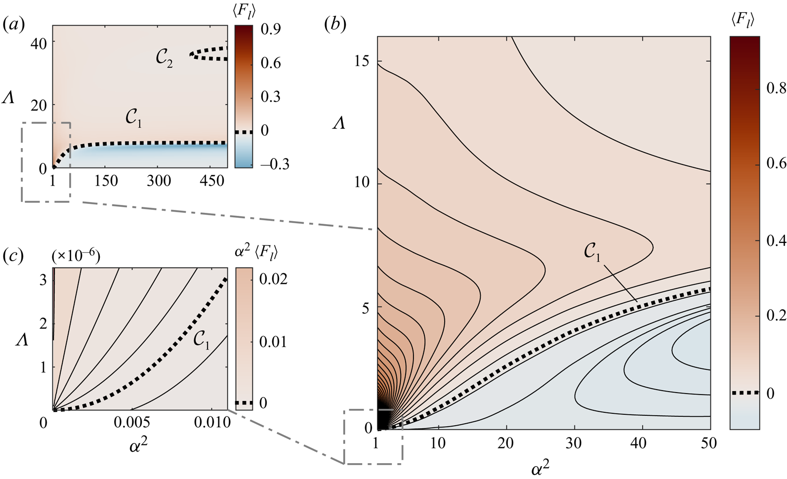
Figure 5. The variation with  $\alpha ^2$ and $\varLambda$ of the time-averaged force $\langle F_l\rangle$ given in (5.11)–(5.12a,b), for $\widehat {{\textit {St}}}=5$ and the piston–wall geometric configuration, with levitative forces $\langle F_l\rangle >0$ coloured red and adhesive forces $\langle F_l\rangle <0$ coloured blue. The computations are carried out using $\nu =0.77$, ${\textit {Pr}}=0.7$ and $\gamma =1.4$. The dotted curves represent contours of zero force $\langle F_l\rangle =0$.
It is natural to note from figure 5(a) that under the classical lubrication limit  $\alpha ^2\to 0$, which has been the subject of thorough investigation for well over a century, the steady squeeze-film force $\langle F_l\rangle$ is levitative for all $\varLambda$ and unaffected by edge flow effects. Figure 6(a) portrays the convergence of the film force, computed with $\widehat {{\textit {St}}}=1$ for the piston–piston edge geometry, to the classical lubrication solution (reported in § 5.3.2) for decreasing values of $\alpha ^2$. The predominance of levitative forces extends also to order-unity values of $\alpha ^2$, provided that the compressibility parameter remains above a critical value $\varLambda _c$, which is larger for larger values of $\alpha ^2$. The value $\varLambda _c(\alpha ^2)$ defines a neutral contour $\mathcal {C}_1$ that marks the transition from levitation to adhesion. Of particular interest is the form of $\mathcal {C}_1$ near the origin of the diagram, which corresponds to weakly compressible systems operating near the lubrication limit. In the associated double limit $\varLambda \ll \alpha ^2\ll 1$, the film force is given by
 \begin{equation} \langle F_l\rangle=\frac{15}{4} \frac{\varLambda}{\alpha^4}+36 \mathcal{P}, \end{equation}
obtained by substitution of (5.26a,b) and (6.20) into  $\langle F_l\rangle =\langle F_i\rangle + A^2 \hat {P_e}$. Correspondingly, for $\alpha ^2 \ll 1$, the critical value $\varLambda _c(\alpha ^2)$, obtained by equating the above expression to zero, exhibits the parabolic dependence
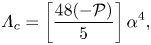 \begin{equation} \varLambda_c = \left[\frac{48 ({-}\mathcal{P})}{5}\right]\alpha^4, \end{equation}
where  $-\mathcal{P} \simeq 2.68 \times 10^{-3}$ for all three geometrical configurations, as reported earlier below (6.20). It is remarkable that this fundamental parametric relation, applicable to squeeze-film systems with relatively low oscillation frequencies, is independent of both the Strouhal number and the specific geometry pertaining to the near-edge region. Using (7.2) together with the definitions given in (1.2) and (1.3) provides
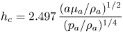 \begin{equation} h_c=2.497 \, \frac{(a \mu_a/\rho_a)^{1/2}}{(p_a/\rho_a)^{1/4}} \end{equation}
for the critical value of the mean gap width at which the force, for such systems, switches from levitation (for  $h_o< h_c$) to adhesion (for $h_o>h_c$).
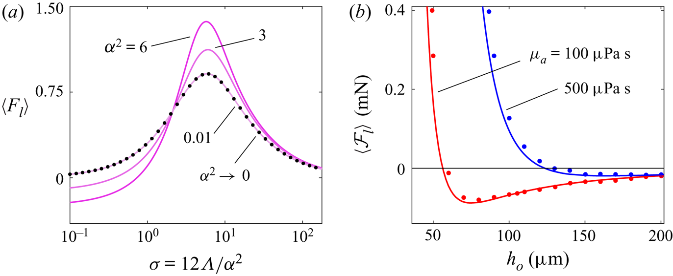
Figure 6. Verification of the predicted steady film force (denoted by solid curves) with (a) the classical limiting lubrication solution obtained from Taylor & Saffman (Reference Taylor and Saffman1957) and (b) time-dependent direct numerical simulations conducted by Andrade et al. (Reference Andrade, Ramos, Adamowski and Marzo2020) (both denoted by dots). For the former case, the dimensionless force is plotted against the squeeze number and for the latter, the dimensional force is plotted against the mean gap width.
The region of the  $\alpha ^2$- $\varLambda$ parametric domain that lies below $\mathcal {C}_1$, which encompasses the strictly incompressible case $\varLambda = 0$, consists entirely of weakly adhesive forces. Interestingly, the dimensionless adhesive force for incompressible squeeze films, to be computed from $\langle F_l\rangle =\langle F_i\rangle + A^2 \hat {P_e}$ with use made of (5.18) and (5.16) to evaluate $\langle F_i\rangle$ and $A^2$, is seen to approach constant limiting values for $\alpha ^2\ll 1$ and $\alpha ^2\gg 1$. In the former case $\alpha ^2\ll 1$, with $\langle F_i\rangle =33/560$, $A=6/\alpha ^2$ and $\hat {P_e}=\mathcal{P} \alpha ^4$, as indicated in (6.20), it follows that
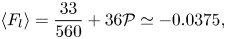 \begin{equation} \langle F_l\rangle = \frac{33}{560}+36\mathcal{P} \simeq{-}0.0375 , \end{equation}
whereas in the latter case  $\alpha ^2\gg 1$, with $\langle F_i\rangle =1/32$, $A=1/2$ and $\hat {P_e}$ approaching its inviscid value $\hat {P_i}(\widehat {{\textit {St}}})$, the solution reduces to
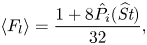 \begin{equation} \langle F_l\rangle = \frac{1+8\hat{P_i}(\widehat{{\textit{St}}})}{32} , \end{equation}
a function of the Strouhal number that is necessarily negative because  $\hat {P_i}$ lies in the range $-1/4<\hat {P_i}<-1/8$, bounded by the limiting values given in (6.23) and (6.28).
As revealed by figure 5(a), the critical value  $\varLambda _c$ defining the contour $\mathcal {C}_1$, the inverse relative acoustic wave speed in the gas film for which the steady pressure variations along the film and near its edge provide cancelling contributions to the film force, is seen to approach a limiting value $\varLambda _\infty$ as $\alpha ^2\to \infty$. This asymptotic behaviour is consistent with the fact that in the limit of nearly inviscid flow, the relative wave speed necessary to produce such a cancellation must cease to depend on viscosity, effects of which are confined to near-wall boundary layers of small relative thickness $\sim \alpha ^{-1} \ll 1$. The region of the parametric domain that lies above $\mathcal {C}_1$ consists largely of levitative forces, but is interrupted by a second neutral contour $\mathcal {C}_2$, which encloses a peninsular region of adhesion that develops for $\alpha ^2 \gtrsim 400$ and $\varLambda \simeq 36$. To determine the value of $\varLambda _\infty$, as well as the possible existence of additional regions of adhesion, it is of interest to evaluate $\langle F_l\rangle =\langle F_i\rangle + A^2 \hat {P_e}$ in the inviscid limit $\alpha ^2\rightarrow \infty$. Using (5.29) and (5.31) gives
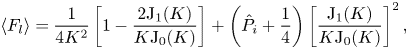 \begin{equation} \langle F_l\rangle=\frac{1}{4K^2} \left[1-\frac{2 \textrm{J}_1(K)}{K \textrm{J}_0(K)} \right]+\left(\hat{P}_i+\frac{1}{4}\right)\left[\frac{\textrm{J}_1(K)}{K \textrm{J}_0(K)}\right]^2, \end{equation}
where  $\hat {P}_i(\widehat {{\textit {St}}})$ is the inviscid value of $\hat {P_e}$ and $K = \sqrt {\varLambda /\gamma }$. The above expression is plotted in figure 7 for selected values of $\hat {P}_i$. As can be seen, the number of zeros, which determines the number of parametric regions of adhesion, depends on the value of $\hat {P}_i$, which in turn is a decreasing function of $\widehat {{\textit {St}}}$ that evolves from $\hat {P}_i=-1/8$ for $\widehat {{\textit {St}}} \ll 1$ to $\hat {P}_i=-1/4$ for $\widehat {{\textit {St}}} \gg 1$. Regardless of the value of $\widehat {{\textit {St}}}$ (i.e. for all values of $\hat {P}_i$ in the range $-1/4 < \hat {P}_i < -1/8$), there always exists at least one zero, which corresponds to the asymptotic value $\varLambda _\infty$ of $\varLambda _c$ as $\alpha ^2 \rightarrow \infty$. As suggested in figure 7(b), this asymptotic value approaches $\varLambda _\infty =0$ for $\widehat {{\textit {St}}}\ll 1$ and $\varLambda _\infty \simeq 8.096$ for $\widehat {{\textit {St}}}\gg 1$, the latter coinciding with the location of the first singularity of (7.6), associated with the first zero of $\textrm {J}_0(\sqrt {\varLambda /\gamma })$ for $\gamma =1.4$. As seen in figure 7(c), two more zeros, bounding the second neutral contour $\mathcal {C}_2$, emerge when the value of $\hat {P_i}$ decreases below $\hat {P_i} \simeq -0.2412$. Additional zeros, which correspond to new regions of adhesion, appear for decreasing values of $\hat {P_i}$ (i.e. increasing values of $\widehat {{\textit {St}}}$), so that, for instance, the existence of a third neutral contour requires $\hat {P_i} \lesssim -0.2466$, as revealed by figure 7(d). The number of zeros diverges as $\hat {P_i}\rightarrow -1/4$ (i.e. as $\widehat {{\textit {St}}} \rightarrow \infty$), creating an infinite cascade of adhesive peninsulas. In this connection, it is worth pointing out that while the existence of the primary neutral contour $\mathcal {C}_1$ for all relevant values of $\hat {P}_i$ (i.e. all finite $\widehat {{\textit {St}}}$ and all three geometries) is a key finding with important consequences for the operation of practical systems, the anticipated relevance of the additional neutral contours $\mathcal {C}_2, \mathcal {C}_3,\dots$ and the corresponding regions of adhesion is somewhat limited, since they only develop for very large values of $\varLambda$.
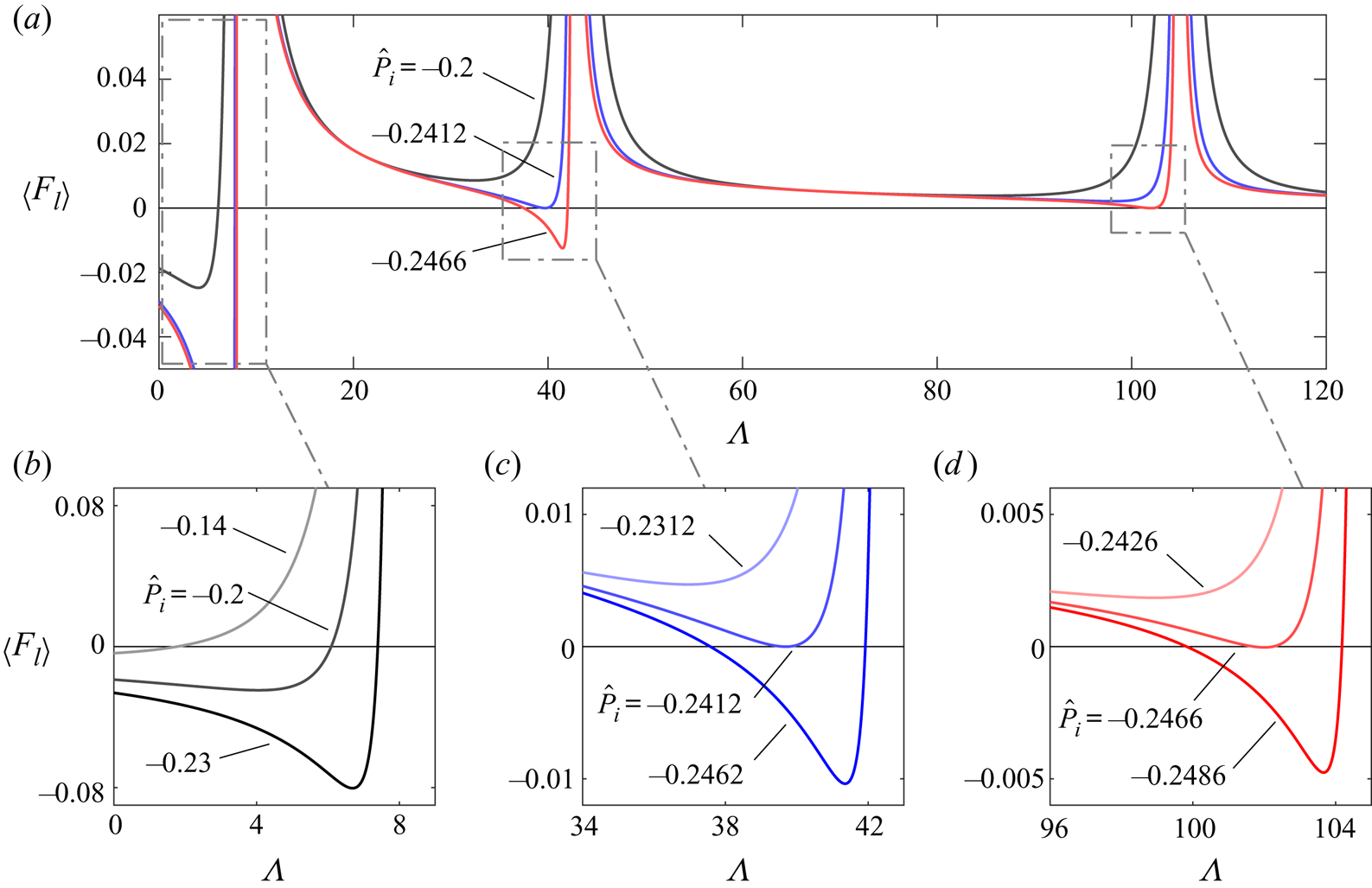
Figure 7. Variation with  $\varLambda$ of (a) the steady squeeze-film force in the inviscid limit (7.6) for different values of $\hat {P}_i(\widehat {{\textit {St}}})$, computed using $\gamma =1.4$. Represented in the bottom row are (b) the first zero of the force, which exists for all $\widehat {{\textit {St}}}$ (i.e. any value of $\hat {P}_i$ in the range $-1/4<\hat {P}_i<-1/8$) and (c,d) subsequent zeros, which emerge for increasing critical values of $\widehat {{\textit {St}}}$ (i.e. decreasing critical values of $\hat {P}_i$ given by $\hat {P}_i\simeq -0.2412,-0.2466,\ldots$).
Recently, time-dependent direct numerical simulations of the piston–piston squeeze-film problem have been conducted by Andrade et al. (Reference Andrade, Ramos, Adamowski and Marzo2020), who found that assuming adiabatic constant-viscosity flow (corresponding to  ${\textit {Pr}}\to \infty$ and $\nu =0$) yields reasonable accuracy relative to their experimental data. In their two-dimensional axisymmetric computations, the dimensional film force $\langle \mathcal{F}_l\rangle$ was quantified for varying mean separation distance and fluid viscosity, while keeping all other dimensional parameters constant. In particular, in terms of the dimensionless governing parameters of our formulation, their operating conditions pertain to the case $0.05 \lesssim \varepsilon \lesssim 0.25$, $2 \lesssim \alpha ^2 \lesssim 65$, $\varLambda \simeq 0.334$ and $0.07 \lesssim \widehat {{\textit {St}}} \lesssim 5.12$. Displayed in figure 6(b) is a comparison of their results with those of the present asymptotic formulation, the latter computed using ${\textit {Pr}}=10^4$ and $\nu =0$, which demonstrates clearly the transition from adhesion to strong levitation when the mean separation width $h_o$ is decreased below its threshold value $h_c$. It must be noted that although the agreement between our theoretical results and the numerical results of Andrade et al. (Reference Andrade, Ramos, Adamowski and Marzo2020) is generally satisfactory, it deteriorates in the levitation regime $h_o < h_c$ because the dimensionless amplitude $\varepsilon$ is no longer small, which compromises the accuracy of the asymptotic predictions.
8. Conclusions
A unifying analytical model of slender axisymmetric gas-lubricated bearings was developed in this study to predict the steady squeeze-film force acting on an axisymmetric rigid body undergoing asymptotically small-amplitude time-harmonic axial oscillations in the vicinity of a parallel surface. Three geometrical configurations involving a disk or a piston as the oscillator and a piston or an infinite wall as the stationary surface were considered as part of the analysis (see figure 1). The method of matched asymptotic expansions was used to relate the Navier–Stokes solutions describing the flow in two distinct regions – a slender region between the parallel surfaces featuring radial flow driven by the disk oscillations and an asymptotically smaller non-slender near-edge region where the motion is driven by said radial flow. The problem was solved in the general case in which the oscillation time is comparable to the three relevant fluid-mechanical times, namely, the characteristic time for radial acoustic-wave propagation, the characteristic viscous time across the gas layer and the characteristic residence time in the near-edge region.
Historically, a major obstacle to computing the viscoacoustic film force has been the determination of a proper boundary condition for the fluid pressure at the edge of the gas layer. The present formulation relies on the distinguished double limit  $\varepsilon \sim \delta \ll 1$ defined by comparable small values of the dimensionless vibration amplitude $\varepsilon$ and the aspect ratio $\delta$, whereby the time-averaged spatial pressure variations across the edge region are comparable to those found along the wall-bounded gas layer. The harmonic leading-order flow inside the slender film was solved analytically, providing a closed-form expression for the radial flow to be used as a matching boundary condition for the near-edge region. Upon computing first-order corrections, the radial departures of the time-averaged pressure inside the gas layer from its value at the edge were found to depend on the Stokes number $\alpha ^2$ and a compressibility parameter $\varLambda$, two order-unity parameters that respectively quantify the relative magnitudes of the viscous and acoustic time scales. Characterizing the near-edge flow required numerical integration of the full Navier–Stokes equations, shown to reduce to their incompressible planar form at leading order, with $\alpha ^2$ and a modified local Strouhal number $\widehat {{\textit {St}}}$ entering as relevant controlling parameters. The dependence on the geometrical configuration was found to be relatively weak, with the magnitude of the pressure drop being slightly larger for wider angles of the near-edge opening of the bounding surfaces.
Our analysis revealed that the time-averaged pressure decreases across the edge region from its value in the stagnant atmosphere and then principally increases along the air gap to reach a local maximum at the axis. These two competing effects determine the sign of the steady dimensionless perpendicular force  $\langle F_l\rangle$ felt by the oscillating body (and also by the stationary parallel surface), so that both attractive and repulsive forces can be generated. The resulting value of $\langle F_l\rangle$ was found to vary strongly with the Stokes number $\alpha ^2$ and the compressibility parameter $\varLambda$, but comparatively weakly with the edge Strouhal number and the geometrical configuration. The typical behaviour of $\langle F_l\rangle$ for a fixed choice of $\widehat {{\textit {St}}}$ and geometry was depicted on a diagram (see figure 5) structured with the principal parameters $\alpha ^2$ and $\varLambda$ as the bounding axes, showing that there is a critical separating contour $\mathcal{C}_1$ in the associated parametric domain across which the steady squeeze-film force switches from positive to negative values, which indicates a transition from repulsion to attraction. The accuracy of the present asymptotic analysis near this transition region was verified by means of comparison with the results of a time-dependent direct numerical simulation conducted recently by Andrade et al. (Reference Andrade, Ramos, Adamowski and Marzo2020) (see figure 6b). It was proven that the contour $\mathcal{C}_1$ exists for all values of $\widehat {{\textit {St}}}$ and different geometrical configurations, and that its shape near the origin is universal, which resulted in an accompanying prediction (7.3) for the critical gap width $h_c$ separating adhesion from levitation for relatively low-frequency squeeze-film systems. The accuracy of this theoretical prediction, in qualitative agreement with the early observations of Popper & Reiner (Reference Popper and Reiner1956) and Taylor & Saffman (Reference Taylor and Saffman1957), should be tested in future work by means of carefully monitored experiments. Also of interest in connection with the force diagram is that additional regions of adhesive force, in the form of peninsulas, develop for large values of the Stokes number $\alpha ^2$ when the value of $\widehat {{\textit {St}}}$ is sufficiently large.
The closed-form analytical expressions provided for the computation of the time-averaged pressure distribution in the slender gas layer as well as the corresponding integral contribution to the steady force, applicable for arbitrary values of the principal parameters  $\alpha ^2$ and $\varLambda$, circumvent tedious numerical computations and expedite the evaluation of the force, a potentially enabling advantage for the operation of high-frequency squeeze-film systems that require real-time feedback control. It is worth pointing out that the analysis of the first-order corrections in the gas film can be readily extended to provide the steady film temperature $\langle \varTheta _1\rangle$ in closed form, if needed in applications. Simplified expressions of the pressure distribution and force for limiting values of $\alpha ^2$ and $\varLambda$ were provided in §§ 5.3 and 7 to allow accelerated computation for systems that operate near the lubrication ( $\alpha ^2\ll 1$), inviscid ( $\alpha ^2\gg 1$) or incompressible ( $\varLambda \ll 1$) limit.
The ability to controllably generate and transition between levitative and adhesive forces using a single squeeze-film system is of significant interest in contemporary applications including acoustic levitation and soft robotics. The construction and assembly-line transport of micro-electronic components would be greatly assisted by acoustic levitation devices capable of suspending sensitive objects from various angles and releasing them on command (see Andrade et al. Reference Andrade, Ramos, Adamowski and Marzo2020). A controllable transition to adhesion is also desirable in the context of contactless locomotion of soft robots over diverse terrains (see Weston-Dawkes et al. Reference Weston-Dawkes, Adibnazari, Hu, Everman, Gravish and Tolley2021). Gaseous squeeze films may be preferable in this context over other adhesive mechanisms such as electromagnetic and dry fibrillar attraction owing to reasons including weight requirements, complexity of manufacturing and limitations in the type of operational surface. The present theoretical study demonstrates that a rigid squeeze-film oscillator can alternate between repulsion and attraction through control of operational variables such as the oscillation frequency and the mean separation width. As previously noted, the closed-form expressions provided in this study may serve to accelerate the feedback response required for the stable operation of such systems.
Practical applicability of the present analysis is limited by the possibility of elastic deformations in the oscillating body that may be non-negligible in the analysis of the induced flow (see Shi et al. Reference Shi, Feng, Hu, Zhu and Cui2019). Of particular interest beyond this study is the characterization of axisymmetric squeeze-film systems involving radially non-uniform driving oscillations  $h=h(r,t)$. In an appendix in their seminal paper, Taylor & Saffman (Reference Taylor and Saffman1957) provided analytical expressions for the mean radial pressure distribution produced by piece-wise linear oscillations $h(r,t)$ of a squeeze-film system in the lubrication limit. Specifically, oscillations of the form $h/h_o=1+\varepsilon (1-2r/a)\cos (\omega t)$, where the mid-circle $r=a/2$ of the disk is fixed and the centre $r=0$ and edge $r=a$ oscillate out of phase, were shown to produce weak adhesive film pressures for low frequencies $\omega$. The ability of smoothly flexible disks to generate stronger adhesive film forces was demonstrated in a recent experimental study by Weston-Dawkes et al. (Reference Weston-Dawkes, Adibnazari, Hu, Everman, Gravish and Tolley2021), where a soft robot equipped with a rapidly oscillating circular disk constructed using plastic shim stock adhered to the bottom surface of a horizontal wall while carrying 35 times its own weight. Comprehension of the physics of such non-rigid high-frequency squeeze-film systems may additionally warrant the modelling of fluid–structure interactions, a problem that should be addressed in future studies.
Acknowledgements
We gratefully acknowledge insightful conversations with Mr W. Weston-Dawkes and Professors M. Tolley and N. Gravish.
Declaration of interests
The authors report no conflict of interest.
Appendix A. Analytical expressions used in the evaluation of the gaseous-film overpressure and its contribution to the steady squeeze-film force
The expressions given in (5.10) and (5.14) involve the complex functions
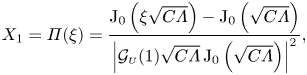 $$\begin{gather} X_1 = \varPi(\xi) = \frac{ \textrm{J}_0\left(\xi{\sqrt{C\varLambda}}\right) - \textrm{J}_0\left({\sqrt{C\varLambda}}\right) }{ \left| \mathcal{G}_{\scriptscriptstyle{U}}(1){\sqrt{C\varLambda}} \, \textrm{J}_0\left({\sqrt{C\varLambda}}\right) \right|^2 } , \end{gather}$$
 $$\begin{gather}X_2 = \frac{ \left| \textrm{J}_1\left(\xi{\sqrt{C\varLambda}}\right) \right|^2 - \left|\textrm{J}_1\left({\sqrt{C\varLambda}}\right) \right|^2 + \displaystyle\int_1^\xi{\dfrac{1}{\xi} \textrm{J}_1\left(\xi{\sqrt{C\varLambda}}\right) \textrm{J}_1\left(\xi{\sqrt{{C^*}\varLambda}}\right) \textrm{d}\xi} }{ \left|\mathcal{G}_{\scriptscriptstyle{U}}(1){\sqrt{C\varLambda}} \, \textrm{J}_0\left({\sqrt{C\varLambda}}\right) \right|^2} , \end{gather}$$
 $$\begin{gather}X_3 = \frac{ {\textrm{J}^*_0}\left({\sqrt{C\varLambda}}\right)-{\textrm{J}^*_0}\left(\xi{\sqrt{C\varLambda}}\right) } { { \textrm{J}^*_0}\left({\sqrt{C\varLambda}}\right) \left| \mathcal{G}_{\scriptscriptstyle{U}}(1)C\varLambda \right|^2} - \frac{ \displaystyle\int_1^\xi{ \textrm{J}_0\left(\xi{\sqrt{C\varLambda}}\right) {\textrm{J}^*_1} \left(\xi{\sqrt{C\varLambda}}\right) \textrm{d}\xi} }{{\sqrt{C\varLambda}} \left| \mathcal{G}_{\scriptscriptstyle{U}}(1){\sqrt{C\varLambda}}\, \textrm{J}_0\left({\sqrt{C\varLambda}}\right) \right|^2} , \end{gather}$$
and the complex constants
 \begin{equation} \mathcal{X}_1 = \frac{{\sqrt{C\varLambda}} - 2\textrm{J}_1\left.\left({\sqrt{C\varLambda}}\right) \right/ \textrm{J}_0\left({\sqrt{C\varLambda}}\right) } {\mathcal{G}_{\scriptscriptstyle{U}}(1) (C\varLambda)^{3/2} } , \end{equation}
 \begin{align} \mathcal{X}_2&=\frac{ \mathrm{i}}{\left| \mathcal{G}_{\scriptscriptstyle{U}}(1) C\varLambda \textrm{J}_0\left({\sqrt{C\varLambda}}\right) \right|^2 } \left\{ \frac{{C^*}\varLambda }{\textrm{Im}(C\varLambda)^2} \textrm{Im} \left[ {\sqrt{{C^*}\varLambda}} \textrm{J}_0\left({\sqrt{C\varLambda}}\right) {\textrm{J}^*_1}\left({\sqrt{C\varLambda}}\right) \right] \right.\nonumber\\ &\quad +\frac{{\sqrt{{C^*}\varLambda}} }{2\,\textrm{Im}(C\varLambda) } \left[ {\sqrt{{C^*}\varLambda}} \left| \textrm{J}_0\left({\sqrt{C\varLambda}}\right) \right|^2 + {{\sqrt{C\varLambda}}} \left| \textrm{J}_1\left({\sqrt{C\varLambda}}\right) \right|^2 \right] \nonumber\\ &\quad\left. +\frac{\textrm{J}_0\left({\sqrt{C\varLambda}}\right) }{\mathrm{i} {\sqrt{{C^*}\varLambda}}} \left[ 2{\textrm{J}^*_1}\left({\sqrt{C\varLambda}}\right) - {\sqrt{{C^*}\varLambda}} {\textrm{J}^*_0}\left({\sqrt{C\varLambda}}\right) \right] \right\} , \end{align}
 \begin{equation} \mathcal{X}_3 =\frac{ \left| \textrm{J}_1\left({\sqrt{C\varLambda}}\right) \right|^2 + \textrm{Im} \left.\left[ {\sqrt{C\varLambda}} \textrm{J}_0\left({\sqrt{C\varLambda}}\right) {\textrm{J}^*_1}\left({\sqrt{C\varLambda}}\right) \right] \right/ \textrm{Im} (C\varLambda) }{\left| \mathcal{G}_{\scriptscriptstyle{U}}(1) {\sqrt{C\varLambda}} \textrm{J}_0\left({\sqrt{C\varLambda}}\right) \right|^2 } , \end{equation}
calculated using the tabulated integrals from Rosenheinrich (Reference Rosenheinrich2012), and
 \begin{equation} \mathcal{H}_1 = 1 - \frac{\tan(\beta_{\scriptscriptstyle{U}}) }{\beta_{\scriptscriptstyle{U}}} , \end{equation}
 \begin{equation} \mathcal{H}_2 = 1 - \frac{\tan(\beta_{\scriptscriptstyle{U}}) }{\beta_{\scriptscriptstyle{U}}} - \frac{\tan(\beta_{\scriptscriptstyle{\varTheta}}) }{\beta_{\scriptscriptstyle{\varTheta}}} - \frac{\beta_{\scriptscriptstyle{U}}\tan(\beta_{\scriptscriptstyle{U}})-\beta_{\scriptscriptstyle{\varTheta}}\tanh(\beta_{\scriptscriptstyle{\varTheta}}) }{\beta_{\scriptscriptstyle{U}}^2+\beta_{\scriptscriptstyle{\varTheta}}^2 } , \end{equation}
 \begin{align} \mathcal{H}_3 &= \frac{ 2\beta_{\scriptscriptstyle{U}} - 2\tan(\beta_{\scriptscriptstyle{U}}) }{\beta_{\scriptscriptstyle{U}} } + \frac{ 2\beta_{\scriptscriptstyle{U}} }{\beta_{\scriptscriptstyle{U}}^2+\beta_{\scriptscriptstyle{\varTheta}}^2 } \left[\vphantom{\frac{\left( \beta_{\scriptscriptstyle{U}}^2-\beta_{\scriptscriptstyle{\varTheta}}^2 \right) \tan(\beta_{\scriptscriptstyle{U}}) + 2\beta_{\scriptscriptstyle{U}}\beta_{\scriptscriptstyle{\varTheta}}\tanh(\beta_{\scriptscriptstyle{\varTheta}}) }{\beta_{\scriptscriptstyle{U}}^2+\beta_{\scriptscriptstyle{\varTheta}}^2 }} \beta_{\scriptscriptstyle{\varTheta}}\tan(\beta_{\scriptscriptstyle{U}})\tanh(\beta_{\scriptscriptstyle{\varTheta}}) \right.\nonumber\\ &\quad \left. - \beta_{\scriptscriptstyle{U}} + \frac{\left( \beta_{\scriptscriptstyle{U}}^2-\beta_{\scriptscriptstyle{\varTheta}}^2 \right) \tan(\beta_{\scriptscriptstyle{U}}) + 2\beta_{\scriptscriptstyle{U}}\beta_{\scriptscriptstyle{\varTheta}}\tanh(\beta_{\scriptscriptstyle{\varTheta}}) }{\beta_{\scriptscriptstyle{U}}^2+\beta_{\scriptscriptstyle{\varTheta}}^2 } \right], \end{align}
 \begin{equation} \mathcal{H}_4 =\frac{ -4\beta_{\scriptscriptstyle{U}}^3 + 15\left[ \tan(\beta_{\scriptscriptstyle{U}})-\tanh(\beta_{\scriptscriptstyle{U}}) \right] - 6\beta_{\scriptscriptstyle{U}}\tanh(\beta_{\scriptscriptstyle{U}})\tan(\beta_{\scriptscriptstyle{U}}) }{24\beta_{\scriptscriptstyle{U}}^3 } , \end{equation}
 \begin{align} \mathcal{H}_5 &= \frac{1}{12\beta_{\scriptscriptstyle{U}}^3} \left[ \beta_{\scriptscriptstyle{U}}\left( 15-2\beta_{\scriptscriptstyle{U}}^2 \right) + \left( 6\beta_{\scriptscriptstyle{U}}^2-9 \right)\tan(\beta_{\scriptscriptstyle{U}})\right.\nonumber\\ &\quad \left. \vphantom{\left( 15-2\beta_{\scriptscriptstyle{U}}^2 \right) + \left( 6\beta_{\scriptscriptstyle{U}}^2-9 \right)}- 6\tanh(\beta_{\scriptscriptstyle{U}}) - 3\beta_{\scriptscriptstyle{U}}\tanh(\beta_{\scriptscriptstyle{U}})\tan(\beta_{\scriptscriptstyle{U}}) \right] , \end{align}
 \begin{align} \mathcal{H}_6 &={-}\frac{1}{6} + \frac{ 2\beta_{\scriptscriptstyle{U}} + \left( \beta_{\scriptscriptstyle{U}}^2-2 \right) \tan(\beta_{\scriptscriptstyle{U}}) }{2\beta_{\scriptscriptstyle{U}}^3} + \frac{\beta_{\scriptscriptstyle{\varTheta}} - \tanh(\beta_{\scriptscriptstyle{\varTheta}}) }{2\beta_{\scriptscriptstyle{\varTheta}}^3} \nonumber\\ &\quad - \frac{ 1 }{2\beta_{\scriptscriptstyle{\varTheta}}\left( \beta_{\scriptscriptstyle{U}}^2+\beta_{\scriptscriptstyle{\varTheta}}^2 \right) } \left[\vphantom{\frac{\left( \beta_{\scriptscriptstyle{U}}^2-\beta_{\scriptscriptstyle{\varTheta}}^2 \right) \tanh(\beta_{\scriptscriptstyle{\varTheta}}) -2\beta_{\scriptscriptstyle{U}}\beta_{\scriptscriptstyle{\varTheta}}\tan(\beta_{\scriptscriptstyle{U}})}{\beta_{\scriptscriptstyle{U}}^2+\beta_{\scriptscriptstyle{\varTheta}}^2 }} \beta_{\scriptscriptstyle{\varTheta}} + \beta_{\scriptscriptstyle{U}}\tan(\beta_{\scriptscriptstyle{U}})\tanh(\beta_{\scriptscriptstyle{\varTheta}}) \right.\nonumber\\ &\left.\quad + \frac{\left( \beta_{\scriptscriptstyle{U}}^2-\beta_{\scriptscriptstyle{\varTheta}}^2 \right) \tanh(\beta_{\scriptscriptstyle{\varTheta}}) -2\beta_{\scriptscriptstyle{U}}\beta_{\scriptscriptstyle{\varTheta}}\tan(\beta_{\scriptscriptstyle{U}})}{\beta_{\scriptscriptstyle{U}}^2+\beta_{\scriptscriptstyle{\varTheta}}^2 } \right] , \end{align}
 \begin{equation} \mathcal{H}_7 = \frac{ \beta_{\scriptscriptstyle{U}} \left( 6-\beta_{\scriptscriptstyle{U}}^2 \right) + 3 \left( \beta_{\scriptscriptstyle{U}}^2-2 \right)\tan(\beta_{\scriptscriptstyle{U}}) }{6\beta_{\scriptscriptstyle{U}}^3 } , \end{equation}
 \begin{equation} \mathcal{H}_8 = \frac{ \left( \beta_{\scriptscriptstyle{U}}^2+1 \right) \tanh(\beta_{\scriptscriptstyle{U}}) - \beta_{\scriptscriptstyle{U}} }{2\beta_{\scriptscriptstyle{U}}^3 } . \end{equation}
The symbols  $\textrm {Re}$, $\textrm {Im}$ and the asterisk $*$ represent the real part, imaginary part and conjugate of a complex function, respectively. The definitions of $\beta _{\scriptscriptstyle {U}}$ and $\beta _{\scriptscriptstyle {\varTheta }}$ are given in (4.13) while those of $C$ and $\mathcal{G}_{\scriptscriptstyle {U}}(1)$ are given in (4.17).


 Open access