


1. Introduction
The primary aim of the European Union (EU) Common Agricultural Policy (CAP) is to support farmers’ income. The measures taken to achieve this aim are decoupled direct payments from the first pillar of the CAP. Moreover, coupled payments for crop- or livestock-specific outputs are made under the first pillar. Additionally, there are subsidies provided under the second pillar of the CAP to improve competitiveness, environment and land management, as well as economic diversity and quality of life. One of the other main aims of the CAP is to enhance agricultural productivity, changes which are reported by the European Commission (EC, 2018). However, there are no direct measures which are aimed at achieving this goal. Rather as mentioned by Minviel and Latruffe (Reference Minviel and Latruffe2017), the impact of subsidies on technical efficiency is a side effect of these subsidies. Indeed, to fulfill the agreements of the WTO, subsidies in the European Union were mostly decoupled from production due to the Fischler Reform in 2003 to reduce the distortions on agricultural markets caused by these subsidies (Rizov, Pokrivcak, and Ciaian, Reference Rizov, Pokrivcak and Ciaian2013, Cillero et al., Reference Cillero, Thorne, Wallace, Breen and Hennessy2018).
This study aims to analyze whether subsidies have an impact on the technical efficiency of Polish dairy farms and, if they do, then in which direction (positively or negatively). The Polish dairy farm sector is an excellent example to study, since Poland is the main milk producer in the European Union (Parzonko and Bórawski, Reference Parzonko and Bórawski2020). As pointed out by Sobczyński et al. (Reference Sobczyński, Klepacka, Revoredo-Giha and Florkowski2015), two main events have had an influence on the dairy sector in Poland in recent decades: the transformation to a market economy in 1989 and accession to the European Union in 2004. They resulted in a significant drop in the number of dairy farms from 1,831,000 in 1990 to 380,000 in 2013, followed by a decrease in the total herd, from 5 million in 1990 to 2.45 million in 2011 (Sobczyński et al., Reference Sobczyński, Klepacka, Revoredo-Giha and Florkowski2015). Despite a dramatic decrease in herd size, the decline in milk production was relatively small, that is from 15 billion kg (in 1990) to 12.36 billion kg in 2011 (Sobczyński et al., Reference Sobczyński, Klepacka, Revoredo-Giha and Florkowski2015) due to increasing yield per cow. It should be noted that, from 2004 to 2011, the situation in the Polish dairy sector stabilized (the number of farms and the herd size) and production was slowly increasing within the limits permitted by the CAP. Further analysis of regional differences, changes in the milk prices, costs of production, and the competitiveness of Polish dairy sector can be found in Sobczyński et al. (Reference Sobczyński, Klepacka, Revoredo-Giha and Florkowski2015) or Parzonko and Bórawski (Reference Parzonko and Bórawski2020).
Analysis of the impact of subsidies on the technical efficiency of farms is one of the topics most frequently addressed in the empirical literature on agricultural economics. However, our study significantly differs from the vast majority of existing studies and therefore contributes to the literature in four ways.
Firstly, we investigate the impact of subsidies on persistent and transient inefficiency employing the heteroscedastic Generalized True Random Effects model (GTRE), while existing studies mostly investigated the impact of subsidies only on one kind of inefficiency (Cillero et al., Reference Cillero, Thorne, Wallace, Breen and Hennessy2018; Rezitis, Tsiboukas, and Tsoukalas Reference Rezitis, Tsiboukas and Tsoukalas2003; Zhu and Lansink, Reference Zhu and Lansink2010; Zhu, Demeter, and Lansink, Reference Zhu, Demeter and Lansink2012).
Secondly, we use a one-step procedure to estimate the GTRE model, while previous studies of the agricultural sector have mostly employed a multi-step procedure (Bokusheva and Čechura, Reference Bokusheva and Čechura2017; Lien, Kumbhakar, and Alem, Reference Lien, Kumbhakar and Alem2018; Trnková and Žáková Kroupová, Reference Trnková and Žáková Kroupová2020; Addo and Salhofer, Reference Addo and Salhofer2022). From the methodological point of view, using a one-step procedure is important because it makes it possible to conduct a statistical test of the most general model with the nested ones (Colombi et al., Reference Colombi, Kumbhakar, Martini and Vittadini2014, p.124).
Thirdly, we contribute to the empirical literature by checking the robustness of the obtained results concerning technical efficiency scores and the impact of subsidies across competing panel data stochastic frontier models. As pointed out by Oumer et al. (Reference Oumer, Mugera, Burton and Hailu2022), this is rare in studies of the agricultural production sector. To date, apart from Oumer et al. (Reference Oumer, Mugera, Burton and Hailu2022), the other following works that should be mentioned in this strand of literature are Abdulai and Tietje (Reference Abdulai and Tietje2007), Kumbhakar, Lien, and Hardaker (Reference Kumbhakar, Lien and Hardaker2014), and Pisulewski and Marzec (Reference Pisulewski and Marzec2019). However, in the above-mentioned studies only homoscedastic TRE (True Random Effects) or GTRE models were investigated, while we investigate a heteroscedastic generalization of these models.
Fourthly, as pointed out by Minviel and Latruffe (Reference Minviel and Latruffe2017), most studies take total subsidies to be the determinant of inefficiency. Using such an approach, it is impossible to distinguish the effect of particular subsidies, the aim of which can differ greatly. To be able to identify the impact of a particular subsidy, we have defined five separate variables for each type of subsidy, that is, decoupled, coupled, Less Favoured Areas (LFA), environmental, and other rural development subsidies, as the determinants of inefficiency.
In the present study, we consider several competing panel data stochastic frontier models. In particular, we first investigate the homoscedastic SFA model (M1) and compare it with the heteroscedastic model (M2) proposed by Caudill, Ford, and Gropper (Reference Caudill, Ford and Gropper1995), which allows for the study the efficiency drivers. Subsequently, since the heterogeneity of farms in the European Union is often underlined in the literature (Kryszak and Herzfeld, Reference Kryszak and Herzfeld2021), we consider the models which account for the unobserved heterogeneity, that is the homoscedastic True Random Effects (TRE) model (M3) and the heteroscedastic one (M4). Finally, we consider the model which accounts for both unobserved heterogeneity and persistent inefficiency, that is the homoscedastic GTRE model (M5) and its heteroscedastic version (M6). In the present study, we are primarily interested in the determinants of transient and persistent inefficiency. Therefore, we made their variances heteroscedastic as in Lai and Kumbhakar (Reference Lai and Kumbhakar2018). However, Badunenko and Kumbhakar (Reference Badunenko and Kumbhakar2017) have demonstrated that it is possible to make the variances of all components heteroscedastic.
2. Review of Literature on the Link between Subsidies and Efficiency
According to Kumbhakar and Lien (Reference Kumbhakar and Lien2010), three approaches to examining the effects of subsidies on farm performance can be distinguished. In the first approach, subsidies are treated as a traditional input. The second approach analyzes the impact of subsidies on productivity through technical inefficiency. In the third approach, proposed by McCloud and Kumbhakar (Reference McCloud and Kumbhakar2008), subsidies are treated as a facilitating input, thus affecting both technical efficiency and indirectly output by changing the productivity of traditional inputs and shifting the technology. The second approach is the most common in the literature, and there are numerous studies which employ this approach. Since, in the present study, we apply this approach as well, we present a brief review of these studies below, focusing on those concerned with the impact of subsidies on the technical efficiency of dairy farms.
Zhu, Demeter, and Lansink (Reference Zhu, Demeter and Lansink2012) analyzed the effect of subsidies on the technical efficiency of dairy farms in Germany, Netherlands, and Sweden. They defined three subsidy-related variables. The two variables reflecting the effect of coupling are the share of livestock subsidies and input-related subsidies in relation to total subsidies. The third subsidy-related variable is the share of total subsidies in relation to total farm income, which may have an influence on the farmer’s production decisions through a wealth and insurance effect. They found, in each case, that an increase in a subsidy-related variable leads to a decrease in technical efficiency in all three countries.
Sipiläinen, Kumbhakar, and Lien (Reference Sipiläinen, Kumbhakar and Lien2014) studied dairy farms in Norway and Finland over the period from 1991 to 2008. They proxied subsidies as the ratio of total subsidies to return. They found a significant negative association between technical efficiency and subsidies in both countries.
Latruffe et al. (Reference Latruffe, Bravo-Ureta, Carpentier, Desjeux and Moreira2017) employed farm-level panel data on dairy farms from nine diverse Western European Union countries: Belgium, Denmark, France, France, Germany, Ireland, Italy, Portugal, Spain, and the United Kingdom (the study was conducted before Brexit) over an 18-year period (1990–2007). They analyzed the impact of subsidies on technical efficiency using the simple Cobb-Douglas production function model. Moreover, they examined whether the direction of the effect changed after decoupling. In five of the nine countries considered, the subsidies were revealed to be statistically significant (Belgium, Spain, Italy, Portugal, United Kingdom), while in four they were non-significant (Denmark, Germany, France, Ireland). Within the group of countries where subsidies were revealed to be statistically significant, two groups were distinguished. The first of these consists of the countries in which subsidies have a negative effect on technical efficiency over the whole period covered: namely Belgium and the United Kingdom. The second group is made up of the countries in which subsidies have a positive association with technical efficiency: namely Spain and Portugal. In the case of Italy, the subsidies had a negative impact before decoupling and a positive one after decoupling.
Marzec and Pisulewski (Reference Marzec and Pisulewski2017) studied the effect of CAP subsidies on the technical efficiency of Polish dairy farms using a Bayesian approach. They employed the farm-level panel data over the period from 2004 to 2011. In their specification, technical inefficiency is time-invariant. Among the types of subsidies considered, the following ones were proved to be statistically significant: coupled, decoupled, and rural development subsidies. The subsidies were defined as the ratio of total subsidies to gross added value. All of them were found to have a negative impact on the technical efficiency score.
Studies which have employed the GTRE model to analyze technical efficiency in the dairy sector include Skevas, Emvalomatis, and Brümmer (Reference Skevas, Emvalomatis and Brümmer2018b), Baležentis and Sun (Reference Baležentis and Sun2020), Trnková and Žáková Kroupová (Reference Trnková and Žáková Kroupová2020) and Čechura, Žáková Kroupová, and Lekešová (Reference Čechura, Žáková Kroupová and Lekešová2022). The first of the above-mentioned studies employs a Bayesian approach and farm-level data on German dairy farms. Although it accounts for determinants of transient and persistent inefficiency, it did not take subsidies into account among the considered determinants. The second study concerns Lithuanian dairy farms, in which the semiparametric stochastic input distance frontier was estimated with a multi-step procedure. In that study, it was found that subsidies have a negative impact on transient technical efficiency. The study by Trnková and Žáková Kroupová (Reference Trnková and Žáková Kroupová2020) also employs a multi-step estimation procedure and data on dairy farms from 26 EU countries aggregated at regional level. They accounted for total livestock subsidies as the determinant of transient inefficiency and the share of LFA subsidies in relation to total subsidies per livestock unit as the determinant of persistent inefficiency. They found that an increase in total subsidies leads to a decrease in transient technical efficiency. The same results were revealed in the case of LFA subsidies, that is an increase in the share of LFA subsidies causes a decrease in persistent technical efficiency. The last of the above-mentioned studies by Čechura, Žáková Kroupová, and Lekešová (Reference Čechura, Žáková Kroupová and Lekešová2022), which concerns the cereals, dairy and beef sectors in the Czech Republic, does not consider determinants of inefficiency.
An alternative approach to measure short-run and long-run technical inefficiency is the dynamic stochastic frontier model introduced by Ahn and Sickles (Reference Ahn and Sickles2000), who specified an autoregressive process on firm-specific efficiency scores. The formulation of such a model makes it possible to account for the persistence of shocks in firm-level efficiency. Skevas, Emvalomatis, and Brümmer (Reference Skevas, Emvalomatis and Brümmer2018a) applied the above-mentioned dynamic stochastic frontier model to measure the short-run and long-run technical inefficiency of German dairy farms. Moreover, they analyzed the impact of several determinants on long-run technical inefficiency. In particular, they found that subsidies (defined as the total amount of subsidies in thousands of euros) have a negative impact on long-run technical efficiency.
In a subsequent study, Skevas, Emvalomatis, and Brümmer (Reference Skevas, Emvalomatis and Brümmer2018c) investigated not only the determinants of technical efficiency but also the determinants of persistence of inefficiency. They found that subsidies (defined as total subsidies per hectare) contribute to the persistence of inefficiency on German dairy farms.
Finally, McCloud and Kumbhakar (Reference McCloud and Kumbhakar2008) investigated the impact of subsidies on technical efficiency using an approach in which subsidies are treated as a facilitating input. They found a positive impact of subsidies on technical efficiency in Denmark, Finland, and Sweden.
A short review of the existing literature analyzing the impact of subsidies shows that there are only a few studies that consider subsidies to be determinants of transient and persistent inefficiency. Moreover, most previous studies in the agricultural sector have employed a multi-step procedure and define total subsidies as a determinant of inefficiency. However, it is well-recognized in the literature (e.g. Minviel and Latruffe [Reference Minviel and Latruffe2017] or Staniszewski and Borychowski [Reference Staniszewski and Borychowski2020]) that each type of subsidy granted under Common Agricultural Policy has a different aim. Therefore, from a policy-making perspective, it is vital to properly identify the impact of each type of subsidy on transient and persistent inefficiency. For this reason, in the present study, following Colombi, Martini, and Vittadini (Reference Colombi, Martini and Vittadini2017), Martini et al. (Reference Martini, Scotti, Viola and Vittadini2020) and Skevas, Emvalomatis, and Brümmer (Reference Skevas, Emvalomatis and Brümmer2018b), we have defined the same determinants of transient and persistent inefficiency and employed a one-step procedure.
3. Methodology
3.1. Stochastic Frontier Production Function Models
Stochastic frontier models were first proposed by Aigner, Lovell, and Schmidt (Reference Aigner, Lovell and Schmidt1977), as well as Meussen and van den Broeck (Reference Meeusen and van den Broeck1977). Pitt and Lee (Reference Pitt and Lee1981, Model II) generalized this class of models to handle cross-section and time series data by considering the following model (hereafter referred to as the pooled model and denoted in the present study by M1):
 $$y_{it}=h\left(x_{it};\beta \right)+v_{it}-u_{it}$$
where y
it
is the natural log of the observed output for firm i (i = 1,…, N) in time t (t = 1,…,T), h is a known production function, x
it
is the (row) vector of natural logs of inputs used by the firm, β is a (column) vector of k parameters. This production function is usually specified to be log-linear in practice, that is h(x
it
; β) = x
it
· β. Furthermore, v
it
is a normal random error term with a mean of zero and constant variance σ
v
2, representing random shocks, v
it
∼ N(0,σ
v
2) and, consequently, it is constant over individuals and time (homoscedastic). Component u
it
≥ 0 is referred to as inefficiency, and so the output-oriented TE score is calculated as ${\rm TE}_{it}=\mathit{\exp } \left(-u_{it}\right)$
. The conventional assumption is that the error term and the inefficiency term are independently and identically distributed across i and t. In the study by Aigner, Lovell, and Schmidt (Reference Aigner, Lovell and Schmidt1977), the inefficiency term is derived from a normal distribution truncated above at zero, u
it
∼ N
+(0, σ
u
2), or it has an exponential distribution. Other commonly adopted distributions are the truncated normal and gamma distributions (Stevenson, Reference Stevenson1980). This study considers only the models with a half-normal distribution for the one-sided inefficiency component.
${\rm TE}_{it}=\mathit{\exp } \left(-u_{it}\right)$
. The conventional assumption is that the error term and the inefficiency term are independently and identically distributed across i and t. In the study by Aigner, Lovell, and Schmidt (Reference Aigner, Lovell and Schmidt1977), the inefficiency term is derived from a normal distribution truncated above at zero, u
it
∼ N
+(0, σ
u
2), or it has an exponential distribution. Other commonly adopted distributions are the truncated normal and gamma distributions (Stevenson, Reference Stevenson1980). This study considers only the models with a half-normal distribution for the one-sided inefficiency component.
The heteroscedastic version of this model was proposed by Caudill and Ford (Reference Caudill and Ford1993) and Caudill, Ford, and Gropper (Reference Caudill, Ford and Gropper1995). In the present study, following Wang (Reference Wang2002), we parametrized the variance as an exponential function of a linear combination of known covariates:
 $$\sigma _{u,it}^{2}=\exp (z_{u,it}\cdot \gamma _{u})$$
where z u, it is a vector of dimensions 1 × ku that includes a constant term and some additional variables which potentially explain inefficiency and γ u is a column vector of new parameters. The model will hereafter be denoted as M2. To ease the estimation procedure, the homoscedastic case (M1) is obtained using the same parametrization (2) but defining z u, it ≡ 1. The variance of the random noise stays homoscedastic in both models (M1 and M2), but it is parametrized as follows:
 $$\sigma _{v}^{2}=\exp (\gamma _{v,0})$$
where γ v, 0 is a single real parameter.
The subsequently considered model in the present study is the True Random Effects stochastic frontier model, which was proposed by Greene (Reference Greene2005a, Reference Greene2005b). Apart from the random noise and inefficiency, this model includes a third component, which captures the firm-specific effects that are not controlled by some extra explanatory variables and differ from inefficiency. Therefore, this model aims to account for unmeasured heterogeneity, as well as firm time-varying inefficiency. As argued by Greene (Reference Greene2005a, Reference Greene2005b), in the conventional stochastic frontier models inefficiency is confounded with heterogeneity that leads to an overestimation of inefficiency, which effectively means that efficiency scores are underestimated. A number of studies seem to prove this point, for example, Abdulai and Tietje (Reference Abdulai and Tietje2007), Hailu and Tanaka (Reference Hailu and Tanaka2015), Pisulewski and Marzec (Reference Pisulewski and Marzec2019). The above-mentioned model (hereafter referred to as M3) takes the following form:
 $$y_{it}=w_{i}+h\left(x_{it};\beta \right)+v_{it}-u_{it},$$
where the heterogeneous intercept w i is treated as a random variable and represents the effects of unobserved variables specific to firm i in the same fashion over time, w i ∼ N(0, σ w 2). However, in contrast to inefficiency, this random variable can take both positive and negative values. Similarly, as in the case of the M1 model, we consider also the heteroscedastic version of M3, hereafter referred to as M4, by parametrizing the variance of the inefficiency term as in (2). The variance of the random noise v it stays homoscedastic and is parametrized according to (3), while the variance of the firm-specific effects can be parametrized similar to the variance of the distribution of v it :
 $$\sigma _{w}^{2}=\exp (\gamma _{w,0})$$
Moreover, we employed the GTRE model (hereafter referred to as M5) introduced by Colombi (Reference Colombi2010), Colombi, Martini, and Vittadini (Reference Colombi, Martini and Vittadini2011), and Colombi et al. (Reference Colombi, Kumbhakar, Martini and Vittadini2014). The feature of the model distinguished in this study is the inclusion of two types of inefficiency: transient and persistent. Moreover, the model, similarly to the TRE model, includes firm-specific effects (w i ) in the same way as the classical model for panel data. In the case of the stochastic production function, it takes the following form:
 $$y_{it}=h\left(x_{it};\beta \right)+v_{it}-u_{it}+w_{i}-h_{i},$$
where h i ∼ N +(0, σ h 2) is interpreted as a persistent (firm-specific, time-invariant or long run) component of inefficiency and u it is treated as one that varies randomly across firms, as well as over time and represents the transient (short run) part of inefficiency, u it ∼ N +(0, σ u 2). In the present study, we consider what is known as the Heteroscedastic GTRE model (denoted hereafter as M6) proposed by Badunenko and Kumbhakar (Reference Badunenko and Kumbhakar2017). However, unlike in their work, we follow Lai and Kumbhakar (Reference Lai and Kumbhakar2018) and assume that only the variances of transient and persistent inefficiency are heteroscedastic as in (2) and (7), respectively, that is σ u, it 2 is parametrized as before according to (2) while variance of the distribution of persistent inefficiency is defined in the same way:
 $$\sigma _{h,i}^{2}=\exp \left(z_{h,i}\cdot \gamma _{h}\right),$$
where z h, i is a set of additional variables that are constant over time and γ h is vector of parameters which are to be estimated.
The models are numbered in such a way that all even numbers refer to the homoscedastic models, while odd numbers indicate the heteroscedastic ones. The parameters of the M1 and M2 models are estimated using the maximum likelihood estimator (Aigner, Lovell, and Schmidt, Reference Aigner, Lovell and Schmidt1977; Caudill, Ford, and Gropper, Reference Caudill, Ford and Gropper1995). The parameters of the M3, M4, M5, and M6 models are estimated by applying the maximum simulated likelihood (MSL) estimator. The details of the MSL estimator in the case of the M3 and M4-type models are discussed in Greene (Reference Greene2005a, Reference Greene2005b), while those in the case of the M5 and M6 models are presented by Filippini and Greene (Reference Filippini and Greene2016).
We briefly present the details of construction of the likelihood function for the GTRE model below. According to the well-known theorem (Azzalini, Reference Azzalini1985), we know that, in the basic model (1), where the half-normal inefficiency assumption is maintained, after integrating u it out of f(v it , u it ), the error term ϵ it = v it − u it has a marginal skew normal distribution with parameters λ = σ u /σ v and σ = (σ v 2+σ u 2)0.5, that is
 $$f_{\varepsilon }\left(\varepsilon _{it};\lambda,\sigma \right)={2 \over \sigma }\varphi \left({\varepsilon _{it} \over \sigma }\right)\cdot \Phi \left(-{\varepsilon _{it} \over \sigma }\lambda \right),$$
where ϕ() and Φ() are the standard normal density and cumulative distribution functions. This density function allows the likelihood function for observations on N firms to be constructed, using the property that ϵ it = y it − h(x it ; β).
In the GTRE model, the joint distribution of two variables (v it −u it ) and (w i −h i ) constitutes the basis for the construction of the likelihood function. Therefore, in the heteroscedastic case of the GTRE model, that is in model (6) and assuming δ i = w i − h i , it follows that the marginal density of ϵ it = y it − h(x it ; β) (but conditional on δ i ) is given by:
 $$f_{\varepsilon |\delta }\left(\varepsilon _{it}|\delta _{i}\right)={2 \over \sigma _{it}}\varphi \left({\varepsilon _{it}-\delta _{i} \over \sigma _{it}}\right)\cdot \Phi \left(-{\varepsilon _{it}-\delta _{i} \over \sigma _{it}}\lambda _{it}\right),$$
where λ it = σ u, it /σ v and σ it = (σ v 2+σ u, it 2)0.5. From the brief discussion above, it can easily be seen that the probability density function of δ i is also a skew normal distribution with parameters σ δ, i = (σ w 2+σ h, i 2)0.5 and λ δ, i = σ h, i /σ w (see e.g. Colombi et al., Reference Colombi, Kumbhakar, Martini and Vittadini2014, p. 135):
 $$f\left(\delta _{i}\right)=f_{\delta }\left(\delta _{i};\lambda _{\delta,i},\sigma _{\delta,i}\right).$$
To obtain the distribution of ϵ it that is unconditional and so marginal on δ i , which is needed to form the likelihood, the δ i must be integrated out from the joint distribution of (ϵ it , δ i ). Finally, the likelihood function for the firm i in the GTRE model is given by
 $$f\left(y_{i};\theta \right)=\int _{-\infty }^{\infty }\prod _{t=1}^{T}f_{\varepsilon |\delta }\left(\varepsilon _{it}|\delta _{i}\right)\cdot f_{\delta }\left(\delta _{i};\lambda _{\delta,i},\sigma _{\delta,i}\right)d\delta _{i},$$
where vector θ contains all parameters of the model.
Colombi et al. (Reference Colombi, Kumbhakar, Martini and Vittadini2014) demonstrated that, using the properties of Closed Skew Normal distribution, it is possible to give a closed form of the above expression. But this approach requires the use of a multivariate cumulative distribution function and requires one to calculate a probability that a (T + 1)-variate normal random variable belongs to the positive orthant. As a result, it leads to computational complexity.
An alternative approach was taken by Filippini and Greene (Reference Filippini and Greene2016) who suggest to approximate the above likelihood function by using Monte Carlo integration. It requires a random sample to be generated from a non-standard distribution of the form (10). However, the use of a change of variables, w i = σ w W i and h i = σ h, i |H i |, where W i and H i are normally distributed with mean zero and variance one, results in straightforward sampling according to the following scheme: δ i, r = σ w W ir − σ h, i |H ir | for r = 1, …, R. Consequently, in the GTRE model, the simulated likelihood function for the i-th observation takes the form as follows:
 $$L^{S}\left(y_{i};\theta \right)={1 \over R}\sum _{r\,=\,1}^{R}\prod _{t\,=\,1}^{T}{2 \over \sigma _{it}}\varphi \left({\varepsilon _{it}-\delta _{i,r} \over \sigma _{it}}\right)\cdot \Phi \left(-{\varepsilon _{it}-\delta _{i,r} \over \sigma _{it}}\lambda _{it}\right)$$
In the above expression (12), W ir and H ir are primitive draws taken R times from the standard normal distribution. In the present study, we have used 1,500 Halton draws. In this class of models, that is for independent data, the maximum simulated likelihood estimator of θ is obtained by maximizing the sum of the logarithm for all for individual units. The product over observations gives the log likelihood for all N observations. Gradient-based optimization procedures are required to estimate the parameters of the models presented above. The first- and second-order derivatives for the simulated likelihood function are partially provided in Pisulewski and Marzec (Reference Pisulewski and Marzec2019). The performance of the above-mentioned estimator in case of the homoscedastic GTRE model was investigated by Badunenko and Kumbhakar (Reference Badunenko and Kumbhakar2016), while in case of heteroscedastic errors, it was examined by Lai and Kumbhakar (Reference Lai and Kumbhakar2018).
The remaining issue is to predict technical (in)efficiency for a given farm. In the normal half-normal model (1), it is commonly predicted by using the estimator derived by Jondrow et al. (Reference Jondrow, Lovell, Materov and Schmidt1982), which is the conditional expectation given the composed error ϵ it = y it − h(x it ; β), that is given the observations yit and xit , can be obtained as:
 $$E\left[u_{it}|\varepsilon _{it}\right]=\tilde{\mu }_{it}\varepsilon _{it}+\tilde{\sigma }_{it}{\varphi \left(-a_{it}\varepsilon _{it}\right) \over 1-\Phi \left(-a_{it}\varepsilon _{it}\right)},$$
where $a_{it}=\tilde{\mu }_{it}/\tilde{\sigma }_{it},\tilde{\mu }_{it}={-\sigma _{u,it}^{2} \over \sigma _{u,it}^{2}+\sigma _{v}^{2}}$
, and
$a_{it}=\tilde{\mu }_{it}/\tilde{\sigma }_{it},\tilde{\mu }_{it}={-\sigma _{u,it}^{2} \over \sigma _{u,it}^{2}+\sigma _{v}^{2}}$
, and $\tilde{\sigma }_{it}^{2}={\sigma _{u,it}^{2}\sigma _{v}^{2} \over \sigma _{u,it}^{2}+\sigma _{v}^{2}}$
.
$\tilde{\sigma }_{it}^{2}={\sigma _{u,it}^{2}\sigma _{v}^{2} \over \sigma _{u,it}^{2}+\sigma _{v}^{2}}$
.
Technical efficiency is computed as exp (E[(−u
it
)|ϵ
it
]). The alternative estimator suggested by Battese and Coelli (Reference Battese and Coelli1988) predicts technical efficiency as the conditional expectation of ${\rm TE}_{it}$
:
${\rm TE}_{it}$
:
 $$E\left[\exp \left(-u_{it}|\varepsilon _{it}\right)\right]={1-\Phi \left(\tilde{\sigma }_{it}-a_{it}\varepsilon _{it}\right) \over 1-\Phi \left(-a_{it}\varepsilon _{it}\right)}\exp \left(-\tilde{\mu }_{it}\varepsilon _{it}+0.5\tilde{\sigma }_{it}^{2}\right).$$
The two estimators above can be used to estimate technical efficiency from the models M1 and M2, which do not include an additional variable δ i = (w i −h i ).
However, in the models M5 and M6, in which it is assumed that v it − u it = ϵ it − δ i , the use of formulas (13) and (14) requires replacing ϵ it by ϵ it − δ i , and subsequently integrating out δ i by using numerical techniques. In summary, as suggested Lai and Kumbhakar (Reference Lai and Kumbhakar2018), transient (in)efficiency can be estimated from the following simulated counterparts of the above-mentioned estimators:
 $$E^{S}\left[u_{it}|\varepsilon _{it}\right]={1 \over R}\sum _{r=1}^{R}E\left[u_{it}|(\varepsilon _{it}-\delta _{i,r})\right]\,\hat{f}_{i,r }$$
and
 $$E^{S}\left[\exp \left(-u_{it}\right)|\varepsilon _{it}\right]={1 \over R}\sum _{r=1}^{R}E\left[\exp \left(-u_{it}\right)|(\varepsilon _{it}-\delta _{i,r})\right]\hat{f}_{i,r }$$
where $\hat{f}_{i,r}=L_{i,r}^{S}/\sum _{j=1}^{R}L_{i,j}^{S}$
is the weight function representing the likelihood contribution, and L
i, r
S
is the simulated likelihood function for T observations (y
i
) for individual i evaluated at MSL estimates of the model parameters. From the statistical point of view, the above idea can be used to compute estimates of characteristics of the distribution of h
i
. The persistent inefficiency and efficiency can be also predicted from the simulated estimators as suggested by Lai and Kumbhakar (Reference Lai and Kumbhakar2018):
$\hat{f}_{i,r}=L_{i,r}^{S}/\sum _{j=1}^{R}L_{i,j}^{S}$
is the weight function representing the likelihood contribution, and L
i, r
S
is the simulated likelihood function for T observations (y
i
) for individual i evaluated at MSL estimates of the model parameters. From the statistical point of view, the above idea can be used to compute estimates of characteristics of the distribution of h
i
. The persistent inefficiency and efficiency can be also predicted from the simulated estimators as suggested by Lai and Kumbhakar (Reference Lai and Kumbhakar2018):
 $$E^{S}\left[h_{i}|\varepsilon _{it}\right]={1 \over R}\sum _{r=1}^{R}\left\{\mu _{i}^{*}\delta _{i,r}+\sigma _{i}^{*}\left({\varphi \left(-a_{i}^{*}\delta _{i,r}\right) \over 1-\Phi \left(-a_{i}^{*}\delta _{i,r}\right)}\right)\right\}\hat{f}_{i,r }$$
 $$E^{S}\left[\exp \left(-h_{i}\right)|\varepsilon _{it}\right]={1 \over R}\sum _{r=1}^{R}\left\{\left({1-\Phi \left(\sigma _{i}^{*}-a_{i}^{*}\delta _{i,r}\right) \over 1-\Phi \left(-a_{i}^{*}\delta _{i,r}\right)}\right)\exp (-a_{i}^{*}\delta _{i,r}+0.5\sigma _{i}^{*2})\right\}\hat{f}_{i,r }$$
where a
i
* = μ
i
*/σ
i
*, $\mu _{i}^{*}={-\sigma _{h,i}^{2} \over \sigma _{h,i}^{2}+\sigma _{w}^{2}}$
, and
$\mu _{i}^{*}={-\sigma _{h,i}^{2} \over \sigma _{h,i}^{2}+\sigma _{w}^{2}}$
, and $\sigma _{i}^{*2}={\sigma _{h,i}^{2}\sigma _{w}^{2} \over \sigma _{h,i}^{2}+\sigma _{w}^{2}}$
.
$\sigma _{i}^{*2}={\sigma _{h,i}^{2}\sigma _{w}^{2} \over \sigma _{h,i}^{2}+\sigma _{w}^{2}}$
.
Additionally, Lai and Kumbhakar (Reference Lai and Kumbhakar2018) provide the simulated estimator of the marginal effects of z u, it and z h, i on persistent and transient inefficiency, respectively. Accordingly, the simulated estimator of the marginal effects with respect to the j-th additional variable on both types of inefficiency is given by:
 $${\partial E^{S}\left(h_{i}|\varepsilon _{it}\right) \over \partial z_{h,i,j}}={1 \over R}\sum _{r=1}^{R}\hat{f}_{i,r }\gamma _{h,j}{\sigma _{h} \over 2}\left[\left(1+(a_{i}^{*}{\delta _{i,r}})^{2}\right)b_{i,r}^{*}+a_{i}^{*}\delta _{i,r}\left(b_{i,r}^{*}\right)^{2}\right]$$
 $${\partial E^{S}\left(u_{it}|\varepsilon _{it}\right) \over \partial z_{u,it,j}}={1 \over R}\sum _{r=1}^{R}\hat{f}_{i,r }\gamma _{u,j}{\sigma _{u,it} \over 2}\left[\left(1+({a_{it}}{\delta _{i,r}})^{2}\right)\tilde{b}_{it,r}+a_{it}\delta _{i,r}\left(\tilde{b}_{it,r}\right)^{2}\right]$$
where $b_{i,r}^{{\rm *}}={\varphi \left(-a_{i}^{{\rm *}}\delta _{i,r}\right) \over 1-\Phi \left(-a_{i}^{{\rm *}}\delta _{i,r}\right)}$
and
$b_{i,r}^{{\rm *}}={\varphi \left(-a_{i}^{{\rm *}}\delta _{i,r}\right) \over 1-\Phi \left(-a_{i}^{{\rm *}}\delta _{i,r}\right)}$
and $\tilde{b}_{it,r}={\varphi \left(-a_{it}\delta _{i,r}\right) \over 1-\Phi \left(-a_{it}\delta _{i,r}\right)}$
.
$\tilde{b}_{it,r}={\varphi \left(-a_{it}\delta _{i,r}\right) \over 1-\Phi \left(-a_{it}\delta _{i,r}\right)}$
.
In this paper, six models of production function are analyzed and compared. We use the econometric methodology of general-to-specific modeling, in which the modeler simplifies an initially general model that adequately characterizes the empirical evidence within his or her theoretical framework, as per Campos, Ericsson, and Hendry (Reference Campos, Ericsson and Hendry2005).
4. Data on Polish Dairy Farms
The data set retrieved from the Farm Accountancy Data Network (FADN) consists of accounting data from a representative sample of agricultural farms. It contains a subgroup of holdings that reflect the specified three characteristics exemplified in a target population, that is region (location), economic size and type of farming. In this study, it covers farms, whose main source of revenue in the analyzed period was milk production. The analysis is based on balanced panel data from 1,191 Polish dairy farms over the period between 2004 and 2011. Construction of the variables is based on other studies of dairy farms, in which FADN data has been used (see Skevas, Emvalomatis, and Brümmer, Reference Skevas, Emvalomatis and Brümmer2018a, Reference Skevas, Emvalomatis and Brümmer2018b, Reference Skevas, Emvalomatis and Brümmer2018c; Zhu, Demeter, and Lansink, Reference Zhu, Demeter and Lansink2012). It is worth noting that most of the empirical studies on dairy farms cover a similar time period, for example: Čechura et al. (Reference Čechura, Grau, Hockman, Levkovych and Kroupová2017); Cillero et al. (Reference Cillero, Thorne, Wallace, Breen and Hennessy2018); Marzec and Pisulewski (Reference Marzec and Pisulewski2017); Skevas, Emvalomatis, and Brümmer (Reference Skevas, Emvalomatis and Brümmer2018a, Reference Skevas, Emvalomatis and Brümmer2018b, Reference Skevas, Emvalomatis and Brümmer2018c); and Baráth, Ferto, and Bojnec (Reference Baráth, Ferto and Bojnec2018). The results on the effect of subsidies obtained in the present study are thus comparable with the ones in the above-mentioned works.
All monetary values have been deflated (at 2004 prices) using price indices provided by Central Statistical Office of Poland for many specific categories, that is the appropriate detailed price indices of non-consumer goods and services. The output (denoted in this study by Q) is specified as the deflated total net farm revenues from sales (FADN code: SE131) excluding the value of feed, seeds, and plants produced on the farm, and, for this purpose, the three price indices of agricultural production were applied. Five categories of input are used in the model:
-
1. Buildings and machinery (K) are measured in terms of deflated book value. This category includes fixed capital such as buildings and fixed equipment (SE450), as well as machines and irrigation equipment (SE455). In this case, the following deflators were used: price index of construction materials, price of repair and construction services, and machinery and equipment for agriculture.
-
2. Total labor (L) is measured in hours. Both hired and family labor declared by the farmer during the interview is included in this measure (SE011).
-
3. Total utilized agricultural area (A, in hectares) refers to owned and rented land (SE025).
-
4. Materials and services (M) are calculated as the sum of several subcategories: purchased feed, seeds and plants, fertilizers, crop protection, crop- and livestock-specific costs and energy (SE281, SE336). It is worth noting that in order to calculate the real value of the expenditure figures, it has been applied five price indices of each item of the input. Moreover, we excluded the value of feed produced within the farm from this category to avoid measuring these costs twice.
-
5. Dairy cows (S) are expressed in standardized livestock units (SE085).
In the present study, we are interested in the impact of subsidies on the technical efficiency of Polish dairy farms. Since the aim of each subsidy is different, we therefore defined several separate subsidy-related variables reflecting the effect of each type of subsidy. In particular, the following five types were distinguished: Coupled subsidies, Decoupled subsidies (SE630), Environmental subsidies (SE621), Less Favored Area subsidies (SE622), and Other rural development subsidies (SE623). The first type of subsidies (coupled) is reported as the sum of items which are directly connected with production, that is total subsidies on crops (SE610), total subsidies on livestock (SE615), subsidies on intermediate consumption (SE625), and subsidies on external factors (SE626).
The second issue with subsidy-related variables is the way they are defined. Generally, the subsidies are treated as exogenous. However, an inappropriate definition can lead to problems with endogeneity. For example, in many previous studies, the variable that reflects the impact of subsidies is usually defined as the ratio of subsidies or the specific type of subsidy to the gross farm income/revenue/total output (Bojnec and Latruffe, Reference Bojnec and Latruffe2009, Reference Bojnec and Latruffe2013; Zhu and Lansink, Reference Zhu and Lansink2010; Zhu, Demeter, and Lansink Reference Zhu, Demeter and Lansink2012). However, proxying the subsidy-related variables by ratio to a production-related variable is criticized by Wang and Schmidt (Reference Wang and Schmidt2002) and by Alvarez et al. (Reference Alvarez, Amsler, Orea and Schmidt2006) as this causes problems with endogeneity. Moreover, Minviel and Latruffe (Reference Minviel and Latruffe2017) stressed that proxying the subsidies by the ratio of these subsidies to farm revenues increases the probability of obtaining a significantly negative effect of subsidies on the farm’s technical efficiency.
The other way of defining the variable that measures the dependence on subsidies is expressing it as the level of subsidies received (Skevas, Emvalomatis, and Brümmer, Reference Skevas, Emvalomatis and Brümmer2018a). However, this method may lead to problems with distinguishing between the size effect and the subsidy effect, since larger farms generally receive more subsidies. Therefore, in the present study, we have adopted the method presented by Latruffe et al. (Reference Latruffe, Bravo-Ureta, Carpentier, Desjeux and Moreira2017), Cillero et al. (Reference Cillero, Thorne, Wallace, Breen and Hennessy2018) and Skevas, Emvalomatis, and Brümmer (Reference Skevas, Emvalomatis and Brümmer2018b), that is, subsidies are expressed in thousands of PLN per hectare.
The descriptive statistics of the models’ variables (over the farms and years) are shown in Table 1. In particular, the table indicates that 25% of farms (in a given year) did not receive any subsidies other than decoupled subsidies, while in 11% of cases no subsidies were reported. Moreover, it should be noted that only 5% of dairy farms (in a given year) received environmental subsidies amounting to more than 200 PLN per hectare, while other rural development subsidies were reported in 3.3% of cases.
Table 1. Summary statistics for the sample farms: average (per annum) value of output, inputs and subsidies for the period from 2004 to 2011

Note: Figures in PLN were deflated (with base year 2004) using price indices.
Source: Own calculations based on FADN Poland.
Table 2. Estimates of the parameters and standard errors from the homoscedastic models
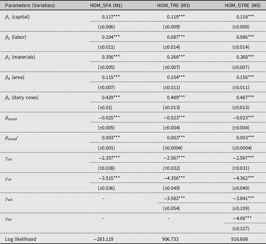
***significant at 0.01 level, **significant at 0.05 level, *significant at 0.10 level.
Additionally, averaging the observations over time shows that the following percentages of dairy farms received the given types of subsidies at least once in the period covered: coupled subsidies - 97%, decoupled subsidies - 100%, environmental subsidies - 28%, LFA subsidies - 77%, other rural development subsidies - 10%.
In conclusion, Polish dairy farms mainly receive three types of subsidies: coupled, decoupled, and LFA subsidies, while environmental and other rural development subsidies are rarely granted to dairy farms. Regarding the dynamics of change, it should be noted that in the first 2 years after accession to the EU only around 57% of dairy farms received any subsidy, while, in the subsequent years, it was around 94% of farms.
5. Empirical Results
The present study uses the translog production function with a quadratic trend component. It belongs to the family of flexible functional forms (Christensen, Jorgenson, and Lau, Reference Christensen, Jorgenson and Lau1973), which are widely used in applied econometrics including production and cost analysis. In our study, the deterministic kernel of the stochastic production frontier is given in this form (in this study, there are four production factors, that is J = 4):
 $$\begin{gathered}
h\left( {{x_{it}};\beta } \right) = {\beta _0} + \sum\nolimits_{j{\kern 1pt} = {\kern 1pt} 1}^J {\beta _j^{\left( t \right)}} {x_{it,j}} + \sum\nolimits_{j{\kern 1pt} = {\kern 1pt} 1}^J {\sum\nolimits_{g \geq j}^J {{\beta _{j,g}}} {x_{it,j}}{x_{it,g}}{\mkern 1mu} + {\beta _{trend}}\cdot + {\beta _{tren{d^2}}}\cdot{t^2}} \\
\beta _j^{\left( t \right)} = {\beta _j} + {\beta _{j,{\text{trend}}}}\cdot\quad {\text{for}}\quad j = 1, \ldots ,J \\
\end{gathered}$$
$$\begin{gathered}
h\left( {{x_{it}};\beta } \right) = {\beta _0} + \sum\nolimits_{j{\kern 1pt} = {\kern 1pt} 1}^J {\beta _j^{\left( t \right)}} {x_{it,j}} + \sum\nolimits_{j{\kern 1pt} = {\kern 1pt} 1}^J {\sum\nolimits_{g \geq j}^J {{\beta _{j,g}}} {x_{it,j}}{x_{it,g}}{\mkern 1mu} + {\beta _{trend}}\cdot + {\beta _{tren{d^2}}}\cdot{t^2}} \\
\beta _j^{\left( t \right)} = {\beta _j} + {\beta _{j,{\text{trend}}}}\cdot\quad {\text{for}}\quad j = 1, \ldots ,J \\
\end{gathered}$$
where the lower case letter x indicates the natural logs of inputs. The present translog form (21) with a linear trend in the parameters is used. The time trend included in the equation above can be treated as an additional input, and, as a result, it allows for non-neutral technical change, that is it raises the productivity of some factors more than others. Alternatively, the advantage of this form is that the elasticities with respect to factors and economies of scale may change over time.
All variables have been mean-corrected prior to estimation. Therefore, the first-order parameters in (21) are interpreted as the output elasticities with respect to the inputs at the geometric mean of the data. These estimates and standard errors of the first-order parameters are presented in Table 2. The obtained results indicate that, in all the considered homoscedastic models, the production elasticity with respect to dairy cows (β
5) is the highest, followed by production elasticity with respect to materials (β
3). The lowest production elasticity is the one with respect to labor (β
2). In the case of production elasticities with respect to area ( $\beta _{4}$
) and capital (β
1), we observe that, in model M1, they are very similar, while in models M3 and M5 the former production elasticity is noticeably higher than the latter. Moreover, the production elasticity with respect to materials is higher in M1 than in models M3 and M5, while the production elasticities with respect to area and dairy cows are higher in models M3 and M5 than in M1.
$\beta _{4}$
) and capital (β
1), we observe that, in model M1, they are very similar, while in models M3 and M5 the former production elasticity is noticeably higher than the latter. Moreover, the production elasticity with respect to materials is higher in M1 than in models M3 and M5, while the production elasticities with respect to area and dairy cows are higher in models M3 and M5 than in M1.
The results obtained with the heteroscedastic models, presented in Table 3, are very similar to the ones obtained with the homoscedastic models (Table 2). In particular, in the “conventional” SF model (M2), the production elasticities with respect to area and capital are again very close. Therefore, in contrast to the homoscedastic models, the order of the production elasticities in the heteroscedastic models is the same. Similarly, as in the case of homoscedastic models, in the heteroscedastic ones, the production elasticity with respect to area is noticeably higher in models M4 and M6 than in M2. Moreover, the production elasticity with respect to materials is again lower in M4 and M6 than in M2. Furthermore, it is worth noting that the parameter estimates of homoscedastic models do not differ much from the ones of their heteroscedastic counterparts. The individual estimates of γ ul for l = 1, …, k u and γ hm for m = 1, …, k h parameters themselves are not interpretable but a sign of a coefficient provides information about the direction of the impact of one subsidy on the inefficiency. Due to the scaling property (Alvarez et al., Reference Alvarez, Amsler, Orea and Schmidt2006; Wang and Schmidt, Reference Wang and Schmidt2002), the absolute values of the above-mentioned estimates may constitute a ranking of the impact of these factors.
Table 3. Estimates of the parameters and standard errors from the heteroscedastic models

***significant at 0.01 level, **significant at 0.05 level, *significant at 0.10 level.
Table 4 presents the results from the comparisons of models based on the likelihood ratio (LR) test. The test statistic has a chi-bar-square distribution (Coelli, Reference Coelli1995; Kodde and Palm, Reference Kodde and Palm1986). First, we tested the homoscedastic models against its heteroscedastic counterparts. In all three cases, the homoscedastic models were rejected. Subsequently, we tested models without random farm effects against the models which account for heterogeneity. We found that the models without random farm effects were rejected. Then, we tested the homoscedastic and heteroscedastic models which include random farm effects but with no persistent inefficiency against the models which account for both heterogeneity and persistent inefficiency. The tests rejected the models without persistent inefficiency, and so the hypothesis that γ h1 = ... = γ h5 = 0 is not supported by the data. Consequently, the model M6 is the best model out of those considered.
Table 4. Model selection based on LR test

Since in the literature it is common to define total subsidies as determinants of inefficiency, we tested (in the model M6) the hypothesis that the impact of all subsidies is the same. The hypothesis takes the following form, as we tested several linear restrictions simultaneously: H 0: γ u1 = γ u2 = γ u3 = γ u4 = γ u5 versus H 1: ∃i ≠ j γ ui ≠ γ uj . The test statistic obtained is 138.88, the critical value read from the tables of chi-bar square distribution is 8.76. Therefore, at a significance level of 0.05, we reject the null hypothesis that all of the parameters are equal. Similarly, the test for the determinants of persistent inefficiency rejects the null hypothesis that the parameters are equal at the 0.05 significance level. Based on these tests, we can conclude that the impact of each type of subsidy is different and that they therefore should not be defined as one total variable. Subsequently, we addressed the further question as to whether the total effect of subsidies is positive or negative. Therefore, we tested H 0: γ u1 + γ u2 + γ u3 + γ u4 + γ u5 = 0 versus H 1: γ u1 + γ u2 + γ u3 + γ u4 + γ u5 < 0. We found that t-statistic is equal to −0.11, while the critical value for this one-sided test is −1.65; thus, we did not reject the null hypothesis. The total effect of subsidies is equal to zero (is non-significant). Similarly, in the case of determinants of persistent inefficiency, we tested H 0: γ u1 + γ u2 + γ u3 + γ u4 + γ u5 = 0 against H 1: γ u1 + γ u2 + γ u3 + γ u4 +γ u5 > 0. Obtaining t-statistic of 30.11 and critical value 1.65, we rejected the null hypothesis, and therefore, we can conclude that the total effect of determinants of persistent inefficiency is positive and contributes to an increase in inefficiency.
Table 5. The effect of subsidies on technical efficiency - from the perspective of models

One of the main aims of the present study is to identify the impact of subsidies on technical efficiency, an aim which is achieved with the heteroscedastic models. We analyzed the models where only determinants of transient inefficiency are included (in the models M2 and M4), and the other one where both transient and persistent inefficiency determinants are present (M6); see Table 5 for details. Regarding coupled subsidies, we can note that, in all the considered models (M2, M4, M6), they were proven to have a positive impact on transient technical efficiency (i.e. the negative sign of a parameter estimate indicates that a variable can contribute to a decline in inefficiency and therefore to improve efficiency). By contrast, their impact on persistent technical efficiency is non-significant in M6. The second type of subsidies analyzed is decoupled subsidies. Their impact was shown to be non-significant in all the models considered above both on transient and persistent technical efficiency.
The effect of environmental subsidies on transient technical efficiency is non-significant in models M2 and M4. However, in model M6, they are significant and have a positive impact on transient technical efficiency, but a negative impact on persistent technical efficiency. LFA subsidies, like other rural subsidies, were shown to have a negative impact both on transient technical efficiency (in all the models) and on persistent technical efficiency.
Generally, the effect of subsidies is consistent across the models considered, that is when a given subsidy has a particular effect, it is the same in all the models considered. The exception to this rule is that of environmental subsidies, which are non-significant in the models M2 and M4, while they proved to be significant in model M6. Moreover, although they have a positive effect on transient technical efficiency, they have a negative impact on persistent technical efficiency.
Furthermore, in our analysis, we were interested in assessing the magnitude of the impact of the subsidies. Accordingly, Table 6 presents the sample statistics of marginal effects of the determinants of technical inefficiency derived from the best model (i.e. M6). Concerning coupled subsidies, we found that (on average) a 1% increase (i.e. 10 PLN per ha) reduces transient inefficiency by 0.099%, while they have no impact on persistent technical inefficiency.
Table 6. Marginal effects of determinants of persistent and transient inefficiency

The next statistically significant determinant was environmental subsidies, a 1% increase in which results in a reduction in transient inefficiency of 0.017%. Moreover, we found that environmental subsidies have an opposite effect on persistent rather than on transient technical inefficiency, that is a 1% increase results in a 0.070% rise in persistent technical inefficiency.
Furthermore, we examined the impact of LFA and other rural subsidies. The result obtained indicates that a 1% increase in the former type of subsidies results in an increase of 0.083% in transient technical inefficiency, while the latter type causes an increase in transient technical inefficiency of 0.018%. Similarly, a 1% rise in LFA subsidies increases persistent inefficiency by 0.297%, while a 1% increase in other rural subsidies results in a 0.164% rise in persistent technical inefficiency.
As regards the estimated values of efficiencies, we can compare them in several ways: (1) between homoscedastic models, (2) between heteroscedastic models, and (3) between homoscedastic and heteroscedastic models. The comparison of technical efficiency between homoscedastic models shows that the average efficiency from the conventional model, that is, M1, is lower than that from M3 which includes the farm-specific effects. As noted by Pisulewski and Marzec (Reference Pisulewski and Marzec2019), including the real-valued random variable with symmetric distribution around zero, can partly capture inefficiency. Comparing the level of transient technical efficiency (TTE) of the TRE model (M3) to that of the GTRE model (M5), we can see that they are approximately equal. However, persistent inefficiency is also included in the GTRE model. Therefore, to properly compare the technical efficiency from model M3 to model M5, we need to obtain the overall technical efficiency (OTE) from M5. It is calculated as ${\rm OTE}_{it}=E\left[\exp \left(-u_{it}\right)|\varepsilon _{it}\right]\cdot E\left[\exp \left(-h_{i}\right)|\varepsilon _{it}\right]$
. Table 7 indicates that the overall technical efficiency from M5 is lower than the transient technical efficiency from M3 (but, in the case of M3, this is the overall technical efficiency). This is a result which is to be expected, because, as pointed out by Colombi et al. (Reference Colombi, Kumbhakar, Martini and Vittadini2014), the model which ignores persistent inefficiency is likely to produce upward-biased efficiencies.
${\rm OTE}_{it}=E\left[\exp \left(-u_{it}\right)|\varepsilon _{it}\right]\cdot E\left[\exp \left(-h_{i}\right)|\varepsilon _{it}\right]$
. Table 7 indicates that the overall technical efficiency from M5 is lower than the transient technical efficiency from M3 (but, in the case of M3, this is the overall technical efficiency). This is a result which is to be expected, because, as pointed out by Colombi et al. (Reference Colombi, Kumbhakar, Martini and Vittadini2014), the model which ignores persistent inefficiency is likely to produce upward-biased efficiencies.
Table 7. Estimates of technical efficiency scores - summary statistics

With regard to the technical efficiency scores obtained from heteroscedastic models, we again found that the average efficiency score from the models that include the firm-specific intercept is higher than in the models that do not include it. In particular, the technical efficiency score is higher in the heteroscedastic TRE model (M4) than in the “conventional” heteroscedastic model (M2). Finally, the homoscedastic models were compared with its heteroscedastic counterparts. We noted that the technical efficiency score is higher in the latter models. This observation concerns all models.
Following Colombi, Martini, and Vittadini (Reference Colombi, Martini and Vittadini2017) or Martini et al. (Reference Martini, Scotti, Viola and Vittadini2020), we took the logs of the transient, persistent, and total efficiency scores, and we obtained the result that 67% of overall technical inefficiency is due to transient technical inefficiency.
In Figure 1, we show how transient and overall efficiency changed over time. It can be seen that, from 2004 to 2007, transient technical efficiency was growing steadily. In 2008, there was a decline, which deepened in 2009. The rebound from the low level of technical efficiency in 2009 occurred in 2010. It is worth noting that a similar pattern of overall technical efficiency was observed in the case of Polish crop farms (Pisulewski and Marzec, Reference Pisulewski and Marzec2019), where there was also a downturn in 2008, though the rebound was observed earlier, that is in 2009, compared to in 2010 in this case.

Figure 1. Persistent and transient efficiency against overall technical efficiency - the changes over time.
6. Discussion and Implications
The average technical efficiency score obtained from the GTRE model is lower than in the previous studies of Polish dairy farms (Čechura et al., Reference Čechura, Grau, Hockman, Levkovych and Kroupová2017; Marzec and Pisulewski, Reference Marzec and Pisulewski2017 or Makieła, Marzec, and Pisulewski, Reference Makieła, Marzec and Pisulewski2017). However, the above-mentioned studies distinguish only one type of inefficiency.
We found that, on average, 67% of total inefficiency is due to the existence of transient technical inefficiency. Therefore, transient inefficiency is the main factor in reducing overall technical efficiency. In the literature, there are mixed results as to which type of inefficiency is the dominant factor in total inefficiency. For example, Skevas, Emvalomatis, and Brümmer (Reference Skevas, Emvalomatis and Brümmer2018c), using the GTRE model, found that 69% of the total inefficiency of German dairy farms is due to persistent technical inefficiency. Similarly, Trnková and Žáková Kroupová (Reference Trnková and Žáková Kroupová2020), based on the regional FADN data on dairy farms from 26 EU countries found in each case that transient technical efficiency is higher than persistent technical efficiency. However, Baležentis and Sun (Reference Baležentis and Sun2020), in the case of Lithuanian dairy farms, found that 63% of total inefficiency comes from transient technical inefficiency. Similarly, Čechura, Žáková Kroupová, and Lekešová (Reference Čechura, Žáková Kroupová and Lekešová2022) reported greater transient technical inefficiency than persistent technical inefficiency for the Czech dairy sector.
In our study, we found that the joint impact of subsidies on transient technical inefficiency is non-significant, while Baležentis and Sun (Reference Baležentis and Sun2020) found that an increase in support payments would increase transient inefficiency. A similar result, though using a model with only one kind of inefficiency (time-varying), was obtained by Latruffe et al. (Reference Latruffe, Bravo-Ureta, Carpentier, Desjeux and Moreira2017) for dairy farms in Denmark, Germany and France. Moreover, our study revealed that an increase in all types of subsidies would lead to an increase in persistent inefficiency. This result is in line with Skevas, Emvalomatis, and Brümmer (Reference Skevas, Emvalomatis and Brümmer2018a), who found a negative effect of subsidies on long-run technical efficiency in the case of German dairy farms.
It is worth noting that other studies that have used the GTRE model, and, while concerned with crop farms, have also reported finding subsidies to have a negative impact. In particular, Minviel and Sipiläinen (Reference Minviel and Sipiläinen2021) analyzed the persistent and transient technical inefficiency of French mixed crop-livestock farms. They defined total subsidies per hectare as the determinant of both persistent and transient inefficiency. In both cases, they found a significant and positive link between subsidies and technical inefficiency, and therefore, they also showed total subsidies to have a negative impact on transient and persistent technical efficiency. Addo and Salhofer (Reference Addo and Salhofer2022), who analyzed Austrian crop farms, found total subsidies to have a negative impact on transient efficiency. However, Lien, Kumbhakar, and Alem (Reference Lien, Kumbhakar and Alem2018) obtained a result which indicated that subsidies have a positive impact on technical efficiency.
Regarding the impact of particular types of subsidies, we did not find any studies, which analyze the impact of different types of subsidies on transient and persistent technical inefficiency in dairy sector. One exception is the study by Trnková and Žáková Kroupová (Reference Trnková and Žáková Kroupová2020). They accounted for total livestock subsidies as the determinant of transient inefficiency and share of LFA subsidies in relation to total subsidies as the determinant of persistent inefficiency. We therefore attempted to compare our results with the ones obtained in previous studies. However, due to the significantly different model specification employed in the present study (two kinds of inefficiency in one model) than in the former ones (only one kind of inefficiency), this had to be done with great caution, that is we compared the marginal effects for the determinants of transient technical inefficiency with the results of the studies where technical efficiency was specified as varying over time. Similarly, we compared the marginal effects for the determinants of persistent technical inefficiency with the results of the studies where technical inefficiency was assumed to be time-invariant.
The first finding regarding the positive impact of coupled subsidies on transient technical efficiency contradicts the results of Zhu, Demeter, and Lansink (Reference Zhu, Demeter and Lansink2012) or Trnková and Žáková Kroupová (Reference Trnková and Žáková Kroupová2020), who found coupled subsidies to have a negative impact on technical efficiency (in the former study, only one kind of inefficiency was specified—transient/time-varying, while, in the latter study, two kinds of inefficiency were specified, but livestock subsidies were a determinant only of transient inefficiency). Similarly, Cillero et al. (Reference Cillero, Thorne, Wallace, Breen and Hennessy2018) showed that coupled subsidies (referred to as “Post-2008 beef subsidies”) cause an increase in technical inefficiency in the case of the subsample (other cattle) of Irish beef farms (in their specification, inefficiency is time-varying/transient).
Regarding the effect of coupled subsidies on persistent technical inefficiency, the results obtained contradict the findings of Marzec and Pisulewski (Reference Marzec and Pisulewski2017), who found that coupled subsidies have a negative impact on (overall, in their specification, persistent/time-invariant) technical efficiency.
Our study shows that an increase in environmental subsidies would lead to a decrease in transient technical inefficiency. This result is in line with Cillero et al. (Reference Cillero, Thorne, Wallace, Breen and Hennessy2018), who obtained a similar result for Irish beef farms. This result is in contrast to the one obtained by Lakner (Reference Lakner2009), who found there to be a negative association between environmental subsidies and technical efficiency (overall, in his specification time-varying) in the case of organic dairy farms in Germany. As noted by Cillero et al. (Reference Cillero, Thorne, Wallace, Breen and Hennessy2018), these payments aim to compensate for the input restriction farmers face to adopt more environmentally friendly practices on farms. Therefore, according to Cillero et al. (Reference Cillero, Thorne, Wallace, Breen and Hennessy2018), a positive effect can arise from the overcompensation in relation to the actual reduction in input use. In the light of the above explanation and the results obtained, it seems that, in the short run, there is overcompensation, but, in the long run, the restrictions on inputs result in lower technical efficiency.
In our study, LFA subsidies were shown to have a significant and negative impact on transient and persistent technical efficiency. A similar result was obtained by Trnková and Žáková Kroupová (Reference Trnková and Žáková Kroupová2020), who showed that an increase in LFA subsidies causes a decrease in persistent technical efficiency. However, these results contradict the conclusions reached by Baráth, Ferto, and Bojnec (Reference Baráth, Ferto and Bojnec2018), who showed that the difference in technical efficiency score between LFA and non-LFA farms is not significant (in their specification inefficiency is time-varying).
Our results concerning other rural development subsidies support the findings of Marzec and Pisulewski (Reference Marzec and Pisulewski2017), who also showed that rural development subsidies have a negative impact on (overall, in their specification persistent/time-invariant) technical efficiency.
The above results enable us to make some policy recommendations. First of all, since overall technical inefficiency is mainly due to transient inefficiency, it would be desirable to implement measures to improve it. Our analysis of the impact of particular subsidies indicates that it is especially LFA and other rural development subsidies that cause market distortions which lead to a decrease in transient technical efficiency. Secondly, although persistent inefficiency is lower than its transient counterpart, it should also be improved. Once again, it is the LFA and other rural development subsidies which are the main contributory factors to an increase in persistent technical inefficiency. In addition to this, environmental subsidies also have a negative impact on persistent efficiency.
7. Conclusions
Most of the models considered indicate the same order of production elasticity with respect to inputs. The highest elasticity is the one with respect to dairy cows, followed by the production elasticities of materials, area, capital, and labor. The exception to this is the simpler model M1, in which the production elasticities of area and capital switch places. Moreover, the results obtained show that including additional random effects (farm effect and/or persistent inefficiency) results in noticeably higher production elasticity with respect to area than in the models without them. By contrast, the production elasticity with respect to materials is higher in the “conventional” SF models (M1 and M2) than in the TRE (M3, M4) or GTRE (M5, M6) models. Based on the comparison of models, we can conclude that the best model is the heteroscedastic GTRE (M6) model in which a 1% increase in input of capital causes a 0.118% increase in production, while, in the case of labor, a 1% increase in this input results in a 0.079% increase in production. A 1% increase in materials leads to a 0.260% increase in production, while a 1% increase in area results in a 0.154% increase in production. The highest elasticity is with respect to dairy cows and a 1% increase in this input results in an increase in production of 0.490%.
The results obtained concerning technical efficiency are consistent between homoscedastic and heteroscedastic models. In particular, both in the homoscedastic and heteroscedastic models, adding farm effects results in an increased mean technical efficiency score. Finally, we found that the mean technical efficiency score is higher in heteroscedastic models than in homoscedastic ones.
It is important for policy makers to know not only the direction of impact but also its magnitude. Our research provides such results. We found that coupled subsidies and LFA subsidies have the greatest impact on transient technical inefficiency. However, the former has a positive impact (reduces inefficiency), while the latter may contribute to an increase in transient technical inefficiency. Similarly, environmental subsidies and other rural subsidies are approximately equal in magnitude, but they work in opposite directions, that is an increase in environmental subsidies decreases transient technical inefficiency, while an increase in other rural subsidies increases transient technical inefficiency. It emerged from an analysis of the marginal effects of determinants of persistent technical inefficiency that LFA, environmental, and other rural development subsidies have a negative impact (increase persistent inefficiency). However, LFA subsidies had the greatest impact, followed by other rural development subsidies, while environmental subsidies had the least impact.
The results obtained show that the impact of each type of subsidy can be different. The present study shows in particular that, while the effect of coupled subsidies is positive in the same model, the impact of decoupled subsidies is non-significant and that of LFA and other rural development subsidies is negative. Therefore, in our opinion, studies which aim to analyze the impact of subsidies on technical efficiency should distinguish between each type of subsidy, because the objective of each type of subsidy is different.
The other important finding of this research is that the impact of the same type of subsidy on different kinds of inefficiency can be different. In the present study, we obtained such a result in the case of environmental subsidies. They were found to have a positive impact on transient technical efficiency, but a negative impact on persistent technical efficiency.
To conclude, the sources of transient and persistent inefficiency are different and therefore the impact of the same type of subsidy can vary between transient and persistent inefficiency. Without conducting a prior analysis, it is hard to make any firm decision as to which type of inefficiency may be impacted by a given type of subsidy. Therefore, we argue that they should be included as determinants of both kinds of inefficiency.
Our study has some limitations which should be mentioned. Following the well-established and commonly applied methodology on analysis of determinants of inefficiency, we treated the subsidies as exogenous. However, some of the subsidies can be endogenous. To the best of our knowledge, to date, there is no well-grounded methodology that exists to resolve this issue. The other potential limitation of our study concerns the problem of selection bias. This problem is likely to occur in case of environmental subsidies, which are voluntary schemes for those farmers who are willing to adopt environmentally friendly practices. These farmers might be characterized by different features (younger, higher qualified) than the remainder of the sample. Greene (Reference Greene2010) suggested a model which can resolve this problem in the case of “conventional” stochastic frontier models. Applying his methodology to the case of GTRE SF models is beyond the scope of the present study, but it is a problem which we believe could be an interesting potential subject for research in the future.


 Open access