


Introduction
Ice domes in the polar regions have traditionally been considered as locations that are well suited for ice-core drilling to study past climate; horizontal velocities and stresses are very small, so the distortion of stratigraphy by ice flow is very limited, and at a stationary dome age is expected to monotonically increase with depth (Reference Cuffey and PatersonCuffey and Paterson, 2010). In a recent study, Reference Martín, Gudmundsson, Pritchard and GagliardiniMartín and others (2009a) showed that the distribution of age and physical properties of the ice at ice divides and domes are far more complex than previously thought. The reason is the anisotropic nature of ice crystals’ physical properties and the development of a strongly anisotropic crystal-orientation fabric (COF) with time, which influences flow properties of ice in the vicinity of the dome.
The current demand for advanced modeling of ice sheets, for accurate reconstruction of their history and improved estimates of their response to climate change, requires the incorporation of anisotropic properties of flow. The Scientific Committee on Antarctic Research (SCAR) committee for Ice Sheet Mass Balance and Sea Level recommended improving the physical basis of next-generation models by incorporating crystal anisotropy (ISMASS committee, 2004). The correlation between anisotropic fabric changes and climate transitions (e.g. Reference PatersonPaterson, 1991; Reference DurandDurand and others, 2007) emphasizes the valuable information carried by vertical and lateral fabric distributions. A reliable determination of COFs over larger areas (e.g. as required for model validation) has not yet been achieved.
A major shortcoming of the numerical models used to investigate dynamics of ice divides is the lack of in situ data indicating the spatial distribution of COFs. Such data can be provided by ice cores for a one-dimensional vertical section, but often models are also used to estimate age/depth relations in pre-site surveys, to select suitable sites for ice coring. With the application of radio-echo sounding (RES) from the surface of an ice sheet or from airplanes, at a limited number of sites it has been possible to estimate the type of COF at depth (Reference Doake, Corr and JenkinsDoake and others, 2002; Reference Fujita, Matsuoka, Maeno and FurukawaFujita and others, 2003; Reference MatsuokaMatsuoka and others, 2003, Reference Matsuoka, Uratsuka, Fujita and Nishio2004, Reference Matsuoka, Power, Fujita and Raymond2012; Reference Eisen, Hamann, Kipfstuhl, Steinhage and WilhelmsEisen and others, 2007). A problem with COF retrieval from englacial layers observed with RES is an ambiguity in the reflection mechanisms. In addition to changes in COF, RES reflectivity is also sensitive to changes in dielectric conductivity. Therefore, several crossing profiles, multi-frequency or multi-polarization RES measurements are necessary to separate the reflections originating from changes in conductivity and COF. Nevertheless, ambiguities remain. Seismic reflectivity, in contrast, depends directly on wave speed (i.e. elastic properties) and density and is independent of conductivity. Below the firn/ice transition in ice sheets, no strong and sharp changes in density occur, thus leaving changes in seismic wave speed as the only obvious reflection mechanism. This can be linked to changes in COF, as the elastic properties of ice, which determine seismic wave propagation and reflection, are likewise anisotropic (Reference Petrenko and WhitworthPetrenko and Whitworth, 1999, p. 36ff.).
Early results obtained in the 1960s and 1970s by Reference Bentley and CraryBentley (1971) and Reference Kohnen and BentleyKohnen and Bentley (1973) confirmed bulk-ice anisotropy for seismic wave speeds in ice. Observations by Reference HorganHorgan and others (2008) employed reflection seismics to deduce the state of anisotropy in the lower part of the ice of Jakobshavn Isbræ in Greenland, an ice-streaming region where COF is well developed because of basal shear. They interpreted vertical changes in ice-stream COF to be the result of different impurity loading (e.g. dust) in ice from different periods during the last glacial termination and the subsequent deformation history of the ice. In a more recent paper, Reference Horgan, Anandakrishnan, Alley, Burkett and PetersHorgan and others (2011) observe similar englacial reflections at several West Antarctic ice streams, which they interpret as confirming the lateral extent of COF changes. Their observed englacial reflection, caused by COF, is supported by the expected ice dynamics and the observed reflection coefficient.
Here we present results from reflection seismic measurements at Halvfarryggen (Fig. 1), a local ice dome in Dronning Maud Land, Antarctica. This site is envisaged for drilling an ice core within the International Partnership in Ice Core Sciences’ 2k/40k programs (Reference Drews, Martín, Steinhage and EisenDrews and others, 2013). We used two types of seismic sources for the data presented here: explosives placed in shallow boreholes and a truck-mounted Failing Y-1100 vibrator (peak actuator force 120 kN) producing 10 s sweeps from 10 to 100 Hz (Reference EisenEisen and others, 2010).

Fig. 1. The survey area of Halvfarryggen, a local ice dome 120 km south of Neumayer III. (a) TerraSAR-X quick-look image of the survey area. The brightness indicates the amplitude of the backscatter. The image shows that the dome is a triple junction of three ice ridges. The survey area of 2011, marked as a red/yellow cross in the lower right corner, is ∼120km from Neumayer III. Parts recorded with vibroseis are marked red. Yellow marks the part also recorded with explosive seismics. Inset: Location of Halvfarryggen, Antarctica. (b) Zoom-in of the survey area with the shot locations. The crossed lines represent the 2011 seismic survey. Red dots are sweep vibrator locations, and yellow dots, overlying some vibrator locations, mark the explosive locations. The six yellow dots on the gray line just north of the crossing point, represent the survey of 2010.
Field Site
Halvfarryggen is an ice dome to the east of the neighboring Ekstrom Ice Shelf, mainly made up of three ice ridges of ∼40 km length (Fig. 1), which meet at a triple junction close to the summit (Reference Drews, Martín, Steinhage and EisenDrews and others, 2013). The ice thickness reaches ∼910m, corresponding to ∼700ma.s.l. elevation (Reference Wesche, Riedel and SteinhageWesche and others, 2009). Accumulation rates are high and variable. Reference Fernandoy, Meyer, Oerter, Wilhelms, Graf and SchwanderFernandoy and others (2010) estimated an average accumulation of 1257 kg mr-2 a–1, with a standard temporal deviation of 347 kg mr-2 a–1. Reference Drews, Martín, Steinhage and EisenDrews and others (2013) determined a spatial variation of accumulation rates within several ice thicknesses of the dome from 400 to 1670 kg mr-2 a–1 .The average annual surface temperature is –17.9°C.
Close to the ice divide the deviatoric driving stresses for ice flow are very small. Numerical studies have shown that under low-stress conditions the viscosity of ice is significantly higher, leading to a mechanically stiff zone beneath a divide (Reference RaymondRaymond, 1983; Reference Pettit, Thorsteinsson, Jacobson and WaddingtonPettit and others, 2007; Reference Martín, Gudmundsson, Pritchard and GagliardiniMartín and others, 2009a). The high viscosity causes slower compaction and thus an upward arching of the isochrones beneath the ridge crest. This effect was first predicted by Reference RaymondRaymond (1983), and the characteristic features known as Raymond bumps or isochrone arches have been found in several ice divides (see Reference Martín, Hindmarsh and NavarroMartín and others, 2009b, for an overview). As the shape of the distorted isochrones of a Raymond bump stack has a significant impact on the age/depth relation of ice beneath a divide, it is essential to understand the process and its influencing parameters in detail. The amplitude of Raymond bumps depends on various parameters. In addition to accumulation rate, onset of divide flow and surface topography, anisotropic ice rheology appears to be a major factor, which, according to model studies (Reference Pettit, Thorsteinsson, Jacobson and WaddingtonPettit and others, 2007), doubles the amplitude of the isochrone arches. A model study by Reference Martín, Gudmundsson, Pritchard and GagliardiniMartín and others (2009a) investigates the evolution of a Raymond bump stack in combination with deformation-induced fabric development. They find that anisotropy induced by the nonlinear flow close to the divide reaches its maximum beneath the ice ridge and increases towards the bed. The corresponding flow regime shows a vertical ice-flow velocity, reaching a maximum directly beneath the divide, which causes a downward arching of the isochrones in the center of the Raymond bumps developed earlier (central syncline). These features have been observed in radar data, and are known as double (peaked) Raymond bumps (Reference Martín, Gudmundsson, Pritchard and GagliardiniMartín and others, 2009a). The synclines within isochrones at the flanks, which are also frequently observed in radar data and which cause the concave ridge shoulders visible on satellite imagery (Reference Goodwin and VaughanGoodwin and Vaughan, 1995), are also reproduced when effects of anisotropic fabric are included. Reference Martín, Gudmundsson, Pritchard and GagliardiniMartín and others (2009a) suggest that Raymond stacks develop in different stages, with the typical central anticlines or bumps developing first, followed by the flanking synclines and the concave ridge shoulders, and finally the central anticline (the latter two only forming if the ice is anisotropic). They conclude that the presence of a double Raymond bump indicates a fully developed steady-state flow system, with deformation-induced anisotropic ice directly beneath the ridge crest. In the model result, the anisotropy of the fabric changed gradually, both with depth and lateral position, but with a steeper vertical gradient. Ice-core observations and modeling studies show that the ice fabric at zero-flow and transient divides undergoes dynamically induced changes (e.g. Reference Thorsteinsson, Kipfstuhl and MillerThorsteinsson and others, 1997; Reference Wang, Thorsteinsson, Kipfstuhl, Miller, Dahl-Jensen and ShojiWang and others, 2002; Reference Bargmann, Seddik and GreveBargmann and others, 2012). Depending on the stress orientation, crystals’ c-axes can, among other more intricate possibilities, orientate themselves in planes that can have different orientation (girdles, as seen at ice divides), or cones of varying opening angles, the extreme case of which is a vertical single-maximum fabric (Reference GowGow and others, 1997; Reference Thorsteinsson, Kipfstuhl and MillerThorsteinsson and others, 1997). At the surface, the c-axis distribution is random or weakly clustered around the vertical (Reference DiPrinzio, Wilen, Alley, Fitzpatrick, Spencer and GowDiPrinzio and others, 2005). With increasing depth, the COF becomes less random and evolves to anisotropic configurations. At domes, the COF usually becomes a cone, narrowing with increasing depth and finally, often close to the base, switches to a vertical single-maximum fabric distribution simply because, when frozen to the base, ice can only deform through simple shear (Reference Budd and JackaBudd and Jacka, 1989; Reference Cuffey and PatersonCuffey and Paterson, 2010). When the ice fabric is no longer random, the bulk-ice properties are different to isotropic ones.
The degree of anisotropy of physical properties (e.g. rheologic, elastic, electromagnetic and thermal) is determined by the COF. As ice deformation parallel to the basal planes of ice crystals is an order of magnitude easier than perpendicular to them (Reference HobbsHobbs, 1974), the degree of the COF affects the dynamics of the ice and this is not adequately described by isotropic deformation. Similarly, the electromagnetic and elastic wave velocities are affected by the COF. The compressional wave speed parallel to the c-axis of an ice crystal is ∼4-5% higher than perpendicular to it (Reference Bentley and CraryBentley, 1971; Reference Petrenko and WhitworthPetrenko and Whitworth, 1999). For radar, the difference between electromagnetic wave velocity parallel and perpendicular to the c-axis is ∼1% (Reference Fujita, Matsuoka, Ishida, Matsuoka, Mae and HondohFujita and others, 2000). The degree of the COF thus determines the elastic and electromagnetic wave velocities (and thus elastic and electromagnetic impedance) of the bulk ice. A change in COF is a change in elastic or electromagnetic impedance. In this way, anisotropy in rheology affects not only the ice dynamics but can also cause reflections in seismic and radar data (Reference Diez, Eisen, Hofstede, Bohlen, Weikusat and KipfstuhlDiez and others, 2012).
Radar stratigraphy merged with flow modeling studies strongly suggest that an anisotropic COF is present at Halvfarryggen. Airborne RES profiles from Halvfarryggen (Reference Drews, Martín, Steinhage and EisenDrews and others, 2013) show that the isochrones of a Raymond bump develop into a double bump with flanking synclines with increasing depth. These features result from ice becoming anisotropic with increasing depth, as reproduced by the flow model of Reference Martín, Gudmundsson, Pritchard and GagliardiniMartín and others (2009a). As bulk-ice anisotropy has consequences for the ice dynamics, a combined vibroseis/explosive seismic survey was set up, to determine the best survey parameters and to investigate the seismic englacial signatures. We compare results of both source methods and interpret our results in terms of possible underlying physical properties.
Measurements and Analysis
Survey set-up in 2010 and 2011
Three seismic datasets were collected at Halvfarrygen: two explosive seismic surveys of 2010 and 2011 (HRexp2010 and HRexp2011, respectively) and one vibroseis survey of 2011 (HRvib2011). The explosive seismic survey of 2010 is marked by the yellow dots on a gray line in Figure 1b. The vibroseis survey of 2011, marked in red in Figure 1b, was set up as a cross with its center ∼100 m to the east of the 2010 survey. The center of the cross line running north-northeast-\south-southwest was also surveyed with explosives. It is marked with yellow dots on the red cross line in Figure 1b, and we refer to it as HRexp2011. The recording parameters discussed here are summarized in Table 1.
Table 1. Overview of the data acquisition parameters of the three seismic datasets at Halvfarryggen (HR). HRexp2010 is the 2010 explosive survey, HRexp2011 is the 2011 explosive survey and HRvib2011 is the vibroseis survey of 2011
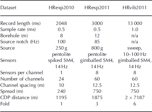
In 2010 we used 24 spiked SM4 14 Hz geophones placed 10m apart and 250g of pentolite explosives (a PETN/TNT mixture) deployed in 8 m deep boreholes. The ghost caused by the charge at 8 m depth gave a source spectral notch of ∼100 Hz. To save time, two shots at different offsets, 25 and 265 m, were detonated in the same borehole (Fig. 2). This effectively doubled the spread length from 240 to 480 m. Boreholes were not tamped, as we used them twice. Both shots were later merged in one shot record with 48 apparent geophones, thus covering 240 m common depth point (CDP) distance, single-fold. After the second shot, the geophones were kept in place while the shot was moved to 265m offset. The data were recorded on a Strataview R24; record length was 2048 ms with a sampling interval of 0.5 ms. A total of 1195 m single-fold CDPs were covered.
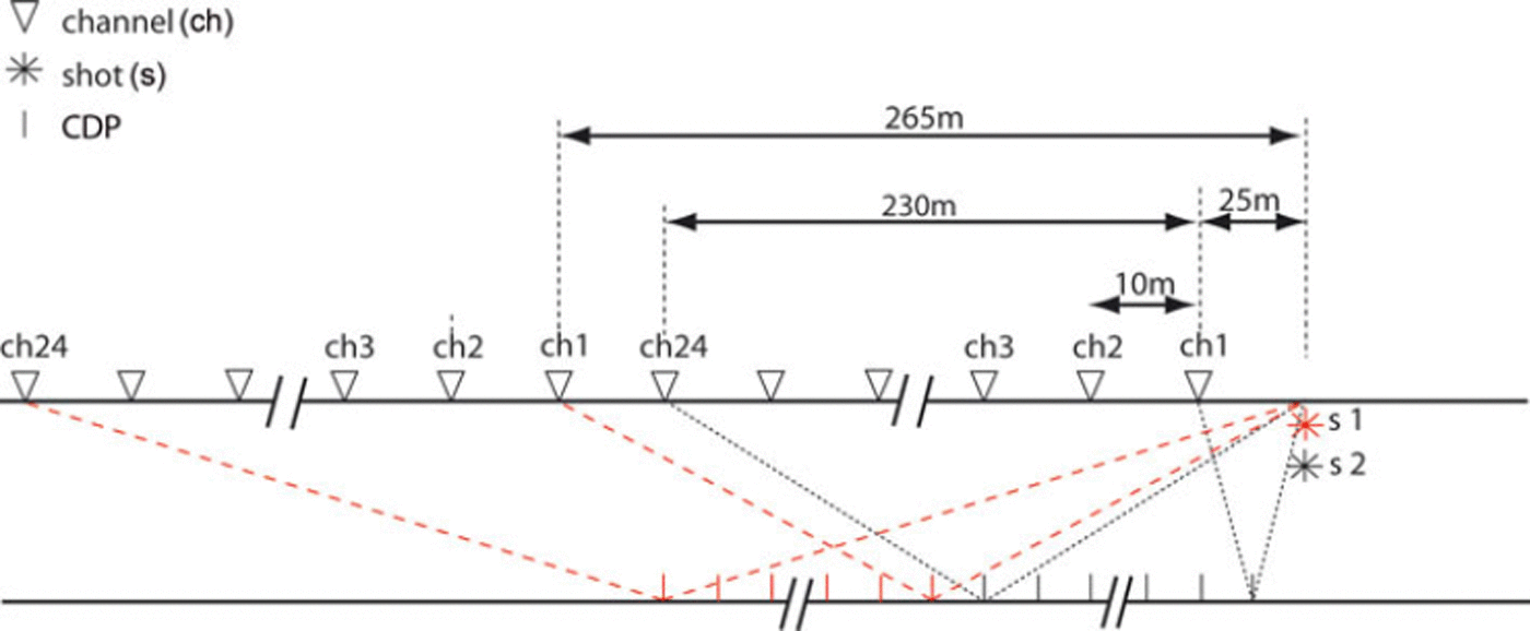
Fig. 2. Seismic set-up of Halvfarryggen in 2010, where we used 24 spiked geophones and explosives in boreholes. Each borehole was used twice at different offsets. Both shots were then merged into one shot record with 48 channels. For the next shot, the geophones were kept in place and the shot location was moved to an offset of 265 m. This way 1195 m CDP distance, single-fold data were recorded.
For recording the 2011 survey (Fig. 1) we used a 60-channel, 1500 m long snowstreamer with a channel spacing of 25 m, similar to the one used by Reference Eiken, Degutsch, Riste and RödEiken and others (1989). A single channel consisted of eight gimballed SM4 14Hz geophones with an effective array length of 25 m (Fig. 3). This streamer is designed for deeper reflections (several kilometers) that arrive at almost vertical incidence (the small-spread assumption). At the base of the glacier at 910 m, the streamer was too long to justify the small-spread assumption. This presented two problems. One problem was that the arrays not only suppressed the surface waves (Reference SheriffSheriff, 1991), but also reflections whose apparent wavelength approached or became smaller than the effective array length. The suppression increases with increasing angle of incidence (offset) and frequency. A second problem was that the large channel spacing causes spatial aliasing. Spatial aliasing also increases with increasing angle of incidence (thus offset) and frequency. Both problems were reduced by towing the streamer in a loop, effectively making the spread 750 m long and decreasing the channel spacing to 12.5 m. As the channels’ array length could not be changed, there still remained some suppression of high-frequency reflections.
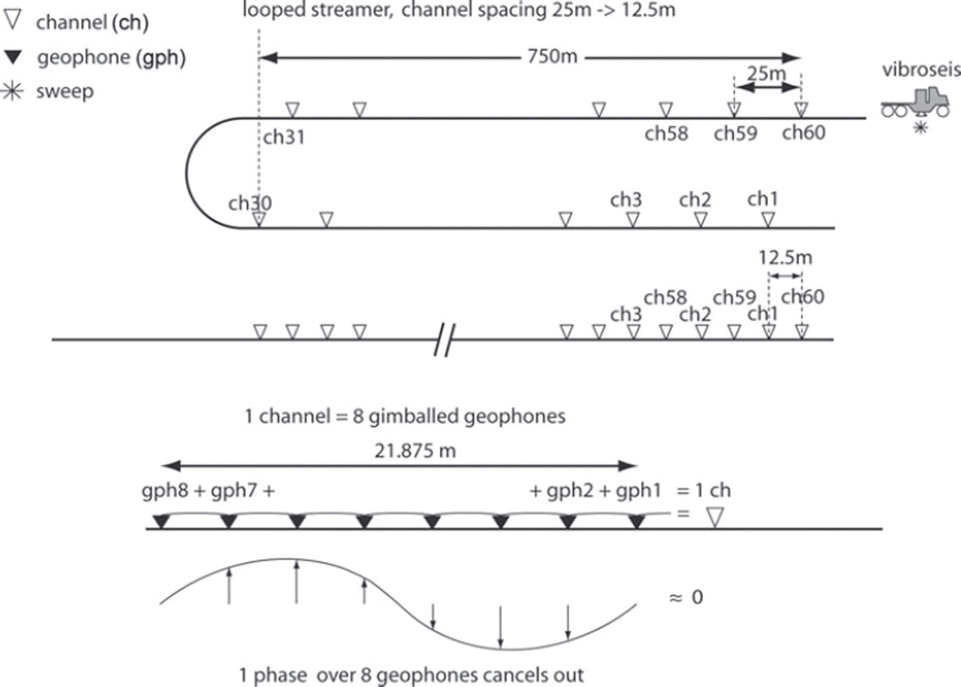
Fig. 3. Vibroseis/streamer set-up: during the survey we towed the 1500 m, 60-channel streamer in a loop. This reduced the streamer length to 750m and the 25 m channel spacing to 12.5 m. The lower picture shows one channel that is built up of eight single geophones in a chain with an array length of 21.875 m, or an effective array length of 25 m (Reference SheriffSheriff, 1991). Though the arrays are designed to suppress ground roll, this has a disadvantage for shallow reflectors. If wavefronts come in at a large angle of incidence, a phase difference over the spread arises, canceling out the signal to some extent. If the phase difference is one cycle, this frequency component of the signal cancels out completely.
For the source we used a truck-mounted Failing Y-1100 vibrator with a weight of 16tons (Reference EisenEisen and others, 2010). The peak actuator force was 120 kN, the base plate area 2 m2, the reaction mass 1769 kg and the stroke 10cm. The truck was mounted on skis, chained to the wheels. A tracked vehicle, a PistenBully 300 (455 HP) pulled the truck-mounted vibrator on skis and a snowstreamer was pulled behind the vibroseis truck. At each location, one sweep was used for compacting the snow, followed by two 10 s sweeps with a linear ramp from 10 to 100 Hz. Sweep locations were 62.5 m apart giving, in combination with the snowstreamer, sixfold data covering 7187 m CDP distance per line. As shown in Figure 1b, two lines of this CDP distance were recorded, one parallel to the main divide to the south (Reference Drews, Martín, Steinhage and EisenDrews and others, 2013) (line 20110551) and one perpendicular to it (line 20110552). The lines crossed in the center near the dome summit. The center of the parallel line was also surveyed with 15 explosive shots. We deployed 800 g pentolite in 12 m deep boreholes, giving a source spectral notch of ∼85 Hz. The shots were 125 m apart, giving a threefold dataset covering 1875 m CDP distance (line 20110501). The data were recorded on a Strataview R60. The record length of the explosives was 3000 ms with a sampling interval of 0.5 ms. The record length of the vibroseis data was 13 000 ms (or 3000 ms of correlated data using the 10 s source sweep) with a sample interval of 1.0 ms.
Vibroseis has been applied successfully in very different glaciological conditions, varying from shelf ice (Reference EisenEisen and others, 2010) to a 4500 m high Alpine saddle (Reference Diez, Eisen, Hofstede, Bohleber and PolomDiez and others, 2013; Polom and others, in press). At Halvfarryggen the vibroseis application was found to be roughly ten times more productive than explosive seismics. Three people performed the entire seismic profiling, with the driver pulling the truck and streamer, and two operators in the truck, one for the vibrator and one for the recording. In this setting, 20 km of CDP sixfold data were easily covered in 1 day. In contrast, drilling holes and deploying explosive charges followed by detonating and recording was much more time-consuming. Five people, in two teams, were needed, two drillers placing the charges and a recording crew of three people. This way 4 km of CDP threefold data were covered per day.
Seismic data analysis
The processing of the three datasets, HRexp2010, HRexp2011 and HRvib2011, is discussed below for each dataset individually. An overview of the processing parameters is given in Table 2.
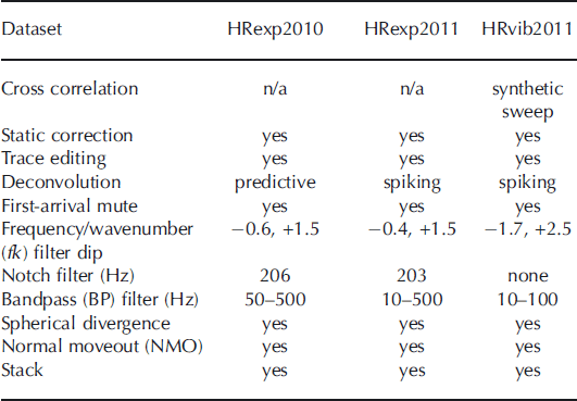
Table 2. Overview of the processing steps of the three seismic datasets at Halvfarryggen (HR). HRexp2010 is the 2010 explosive survey, HRexp2011 is the 2011 explosive survey and HRvib2011 is the vibroseis survey of 2011
Processing of 2010 data
Processing includes first-arrival muting, to remove diving and surface waves, and a notch filter to remove a spurious geophone frequency at ∼206 Hz. To reduce surface waves and diving waves we used both high-pass filtering at 50 Hz and frequency/wavenumber (fk) filtering. The seismic velocity model for the upper part of the ice column was derived from an existing 84 m deep firn core (Reference Fernandoy, Meyer, Oerter, Wilhelms, Graf and SchwanderFernandoy and others, 2010). This provided density data from p = 390 kgm-. 3 at the surface to p = 830 kg m - 3 at 84 m, covering the whole densification from snow to bubble close-off, yielding velocities from 800 to 3650 ms-1, using the Reference KohnenKohnen (1972) approach. The density-derived velocity model was used to compensate for the geometrical spreading. The fk filter worked very well, as all our seismic events within the ice are more-or-less flat and a filter around wavenumber zero suppressed the surface wave and preserved the englacial reflectors. Following Reference SmithSmith (1997) a predictive deconvolution filter was designed and applied to each shot to remove the ghost.
Processing of 2011 data
The vibroseis data were initially cross-correlated with a synthetic sweep, as the vibroseis sweep could not be recorded. The channels were re-sorted as the streamer was towed in a loop. Noisy traces were removed and a first-arrival muting was applied. To increase resolution, spiking deconvolution was applied to both the vibroseis data and the explosive dataset. Applied fk filtering successfully removed the slower ground roll still present at later travel times in the shot record, followed by a 203 Hz notch filter to remove the spurious noise of the SM4 geophone and a 10-500 and 10-100 Hz bandpass filter for the explosive and vibroseis data, respectively. Geometrical spreading was compensated with spherical divergence gain, using the velocity model of the 2010 dataset. The data were normal-moveout corrected and stacked. For the interpretation of the reflectors carried out below, we used a single trace gather of near-offset channel 3 (offset 75 m) that was only bandpass-filtered.
Results and Discussion
Vibroseis Vs Explosive Source
The effect of the different sources and recording channels of the central shot location of the survey is shown in Figure 4. Here three shots created and recorded with different means are compared. The three shots were all triggered within 100 m of the crossing point of the two survey lines.

Fig. 4. Three raw shots acquired by different means within 100 m of the center crossing point of Halvfarryggen. Channel number at the top, increasing with offset from the source. (a) Two explosive shots of the 2010 survey at different offsets merged into one shot record. The shots were recorded with spiked geophones with 250g pentolite in 8 m deep boreholes. Note that englacial reflectors show up throughout the record. (b) Shot from 2011 survey with 800 g pentolite in a 12 m deep borehole using the snowstreamer with geophone arrays for recording. Here, englacial reflections show up more at the near-offset part of the streamer, as the geophone arrays act as a low-pass filter, reducing recorded reflection amplitudes for larger incidence angles (farther offset from shot) at the surface. (c) Vibroseis sweep (10 s, 10–100 Hz) at same location as (b). Although ground roll quite heavily overruns a considerable part of the data, the deepest englacial reflector is clearly visible.
The first shot in Figure 4a is from dataset HRexp2010, consisting of two merged shots, as described above. The strongest reflection occurs at a two-way travel time (TWT) of 0.48 ms. With an average compressional wave speed in ice of 3800 ms-1, we interpret this as the ice/bed contact at 910m depth, which is in accordance with airborne radar observations (Reference Drews, Martín, Steinhage and EisenDrews and others, 2013). Englacial reflections are clearly visible over the whole spread, especially in the upper half of the record. Above the bed reflection, a strong englacial reflector can be seen throughout the shot record, approximately parallel to the bed.
Figure 4b, from dataset HRexp2011, shows the effect of a geophone array used as a single channel. Reflections coming in at large angles (large offsets) cancel out because of the phase difference between the individual geophones of one channel (Fig. 3). As high frequencies have a smaller wavelength, these geophone arrays act as a low-pass filter. The englacial reflections show up mainly in the near offset (first 300 m) of the streamer. Deeper reflectors are also visible at the larger offsets along the streamer.
Figure 4c, from dataset HRvib2011, is a cross-correlated sweep from the vibrator. The motion of the vibrator’s base plate is directional at the surface, exciting vertical particle motion, in contrast to explosives that cause radial particle motion. Whereas much of the energy released during an explosion causes inelastic deformation by breaking ice bonds, i.e. irreversibly destroying the firn, most of the vibroseis energy is purely elastic, i.e. causing wave propagation. However, as the vibroseis excites the waves at the surface, on top of the firn, one would expect poor wave penetration, as firn acts as an energy trap. Its continuous densification with depth causes a diving wave. This is a continuously refracted wave following a curved ray path. Any energy not pointed vertically downward is refracted away from the vertical and a large part comes back to the surface without penetrating below the firn/ice transition.
The limited bandwidth of the sweep reduces the resolution of the seismogram when compared with explosives. Most of the englacial reflections are not visible in the vibroseis data, except for the deepest reflector. The effect of bandwidth filtering on englacial reflections is shown in Figure 5, where we bandpass-filter an explosive shot from dataset HRexp2011 in four steps, reducing the upper cut-off frequency by 100 Hz in each step (10-400, 10-300, 10-200 and 10-100 Hz). The fourth bandpass filter creates a bandwidth comparable to a vibrator sweep (10-100 Hz). Using a bandwidth of 10-400 Hz, the englacial reflections are clearly visible. If the bandwidth is reduced to 10-200 Hz, most englacial reflections lose their visibility. If the bandwidth is 10-100 Hz, comparable to that of the vibroseis data, all englacial reflections disappear, except for the deepest one, which is hard to distinguish from the basal reflector. Clearly, the upper englacial reflectors contain dominant frequencies, >100Hz. The deepest englacial reflection in Figure 5, at TWT 0.45 s, but variable in the range 0.44-0.48s in the explosive datasets HRexp2010 (Fig. 6) and HRexp2011 (Fig. 7c), is also visible with the vibrator but is hard to separate from the basal reflection.
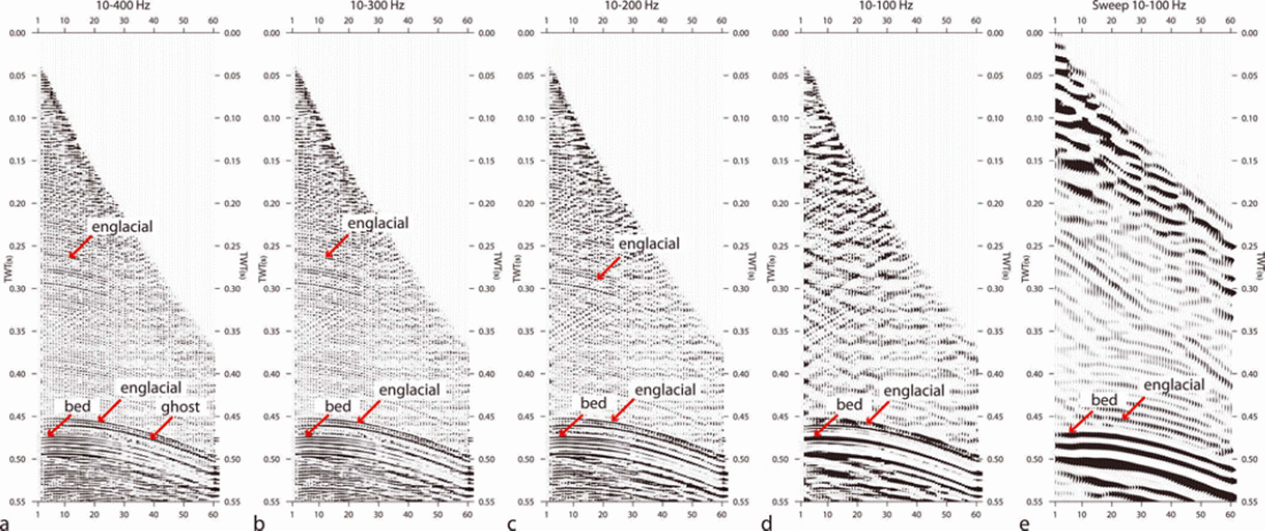
Fig. 5. Analysis of (a–d) a frequency/wavenumber (fk) and bandpass (BP)-filtered explosive shot record and (e) a vibroseis record at the same location, demonstrating the effect of bandwidth on the appearance of englacial reflectors. The shot and sweep have been BP-filtered, as annotated above each panel. The panels show the same explosive shot, whereby the bandwidth reduces in steps of 100 Hz. (d) has a bandwidth of 10–100 Hz, similar to that of the vibroseis data. The englacial reflectors start fading away in (c), with a bandwidth of 10–200 Hz. In (d) only the deep englacial reflector is visible. Note that the ghost is not removed, which is why there appear to be two englacial reflections, one at 0.45 s and the ghost at 0.46 s at this shot location. (e) shows that in the vibroseis data the deep strong englacial reflector is visible, but hardly distinguishable from the basal reflector.

Fig. 6. Single-fold data from 2010, recorded with 24 spiked geophones and 250g pentolite as source. Horizontal axis indicates distance of common depth points (CDP) along the line increasing from south (right) to north (left); vertical axis is two-way travel time (TWT). The seismogram is composed of four shots with 24 channels each. Prominent englacial seismic reflectors (ISR) are highlighted with rose bars underneath and labeled according to their depth TWT (ms) at 0 distance. The two gray-shaded triangles between 0.15 and 0.47 s overlay that part of the data disturbed by spurious signals because of close proximity to the shot location. The presence of at least 11 englacial reflections formed the basis for the more extensive 2011 survey. With a compressional wave speed of 1500 m s–1 in the surface layer and a charge depth of 8 m, the ghost appears 0.01 s after the primary signal with reversed polarity. It is visible after at least three englacial reflectors, IRS218, ISR385 and the deepest englacial reflector, ISR463.

Fig. 7. The two main lines of Halvfarryggen perpendicular to each other in a cross pattern, recorded with vibroseis and the center shot with explosives. (a) Shown here is the vibroseis section that runs west-northwest–east-southeast perpendicular to the main divide (line 20110552). The basal reflector is clearly visible at 0.48 s TWT and also here the englacial reflection is faintly visible above the basal reflector. (b) Vibroseis section parallel to the direction of the southern divide (line 20110551) that runs about north-northeast–south-southwest. Englacial reflected energy is visible above the strong basal reflector at 0.48 s TWT. (c) The center of 20110551 shot with explosives using a 20 ms automatic gain control (AGC) window. In the vibroseis data, only one englacial reflection is visible. The explosive data have a much better resolution and here at least 11 englacial reflections are visible. The reflectors in the explosive data are not as clear as in the 2010 data because they were recorded with geophone arrays instead of spiked geophones. The timing of the englacial reflectors differs from the 2010 dataset, as the datasets are not at exactly the same location.
Interpretation of the 2010 explosive data
The reflection from the base is visible at ∼0.48s TWT, clearly shown for a data subset in Figure 6, a few meters more on the southern than on the northern end. The processed data allow us to clearly identify 11 englacial seismic reflectors (ISR) between 0.18 s TWT and the bed, but there are more, less clear events. The dominant ones are labeled according to their TWT (ms) at abscissa origin, e.g. ISR180 for the uppermost reflector. This corresponds to a depth of ∼300 m, which is significantly below the close-off depth of air bubbles at this site (Reference Fernandoy, Meyer, Oerter, Wilhelms, Graf and SchwanderFernandoy and others, 2010). The lowest englacial reflector, ISR463, is almost parallel to the bed. The depth below the surface of all the ISRs is somewhat lower at the northern than at the southern end of the line. The frequency content of the reflections is high, between 300 and 600 Hz, and the frequency content of the deeper reflectors is somewhat lower (200-500 Hz).
Spurious signals for traces with a shot/geophone offset of less than ∼100m are present in the data (gray-shaded triangles in Fig. 6) and complicate data interpretation of weak ISRs. Especially at larger travel times, these signals inhibit a clear and laterally continuous identification. This is, for instance, the case at line distance 210-235 m and travel times of 0.34-0.48s.
The effect of the ghost (i.e. the delayed source signal which travels from the borehole up to the surface first and then downwards) makes it difficult to unambiguously identify more reflectors. With v = 1500 m s - 1 in the surface layer and a charge depth of 8 m the ghost appears 0.01 s after the primary signal with reversed polarity. This is four times the main period of the source wavelet at a mean frequency of 400 Hz. These characteristics are most obvious for the deepest englacial reflection, ISR463 at 0.46 s, followed by its ghost at 0.47 s TWT
Although the ghost was reduced by the predictive deconvolution, it was not possible to remove it completely. We attribute this to the strong influence of ground roll and other slow events degrading the stationarity of the wavelet signature, relatively low signal-to-noise ratio of englacial events in general (e.g. compared to the basal reflection), as well as the varying angle of incidence. These effects lead to a considerable variation of autocorrelation from trace to trace for short periods.
Interpretation of the 2011 explosive data
Figure 7c displays the central part of line 20110551, shot with explosives. This 1.8 km line is called 20110501. Here we clearly see the same 11 englacial reflectors as in HRexp2010, although in the raw shot records more can be distinguished. As the data were collected by different means (Table 2), some characteristics are not as clear as in HRexp2010. The geophone arrays are less well coupled than the spiked geophones used in HRexp2010. The arrays suppress higher frequencies, and the charge used in both surveys is different (and thus the sources’ frequency content). Nevertheless, the reflectors identified here are also visible in the HRexp2010 dataset. Their timing is somewhat different, but that is because the locations are 100 m from each other. The deepest englacial reflector is clearly the strongest and most continuous, and most likely identical to the one identified in the vibroseis section. It clearly follows the bedrock, and bends slightly towards the bed away from the center in both directions. The amplitudes of the other englacial reflectors vary in strength and are all weaker than the deepest reflector. Occasionally they disappear and reappear.
Interpretation of the vibroseis data
The processed vibrator data for the cross line (20110552) and the parallel line (20110551) are shown in Figure 7a and b, respectively. We interpret the strong reflector with positive polarity between 0.48 and 0.50 s TWT as the base. The phase of the ice/bed reflection is mostly positive throughout the section. This is what we expect, as the base must be frozen as a Raymond bump has developed at Halvfarryggen (Reference Drews, Martín, Steinhage and EisenDrews and others, 2013). Directly above the bed some faint englacial reflected energy is visible in both sections. Although these events appear to follow the basal reflector, they do not do so exactly, so they are at least partly englacial reflections. Also, Figure 5 clearly demonstrates that some englacial reflections are visible in our vibroseis data, but, due to the limited bandwidth, they are hard to separate from the basal reflection. Our interpretation is that the englacial reflection signature shown in the vibroseis data is a combination of poor cross correlation with the synthetic sweep (causing a faint echo) and an englacial reflection. Although the englacial and the bed reflection can be separated in the shot gathers (Fig. 5), they cannot be distinguished in the stacked section. With a 10-100 Hz bandwidth we are at the resolution limit. Above this deepest englacial reflector, the vibrator data do not reveal any englacial reflections.
Origin of englacial reflections
Reflections are caused by contrasts of acoustic impedance, the product of density, p, and compressional wave speed, v. A change in either one or both is needed to cause a reflection. The amplitude and polarity are determined by the reflection coefficient, R, which at normal incidence is given by
where subscripts 1 and 2 refer to two half-spaces and half-space 1 is traversed first. The deepest englacial reflection (Fig. 7c), at ∼0.46s TWT, lies ∼40m above the bed. It appears as a smooth, continuous and coherent reflector. The bed is frozen, and flow modeling indicates stable conditions (Reference Drews, Martín, Steinhage and EisenDrews and others, 2013), making intrusion of subglacial debris unlikely. All englacial reflections are located well below the bubble close-off depth. Therefore, a sufficiently strong change in density is unlikely.
All englacial reflections must, thus, be caused by changes in the compressional wave speed. As we see at least 11 reflectors and we see them throughout the ice column below 0.18 s TWT, we can also exclude wave-speed changes resulting from some kind of temperature change. Abrupt changes (in respect to wavelength) in wave speed must therefore be caused by abrupt changes in elastic properties, and thus COF.
A velocity increase (v 2 > v 1) causes a positive reflection coefficient, and a velocity decrease (v 2 < v 1) a negative reflection coefficient and thus a polarity reversal. As compressional wave speed parallel to the c-axis is ∼5% faster than perpendicular to it, COF will cause a velocity contrast, depending on the rate of change of the c-axesorthe orientation of the cone angle and the variation in opening angles and may cause reflections (Reference Diez, Eisen, Hofstede, Bohlen, Weikusat and KipfstuhlDiez and others, 2012).
Moreover, if a thin layer is embedded in a homogeneous background, the characteristics of the reflected signal recorded at the surface will be the result of interference of the partial reflections from the upper and lower boundary of that layer. If the layer has a thickness less than one-quarter of the wavelength (called tuning thickness in seismics), this interference will be constructive and the reflections will be indistinguishable. The tuning thickness in ice for a frequency of 100 Hz is ∼13.5m (e.g. Reference SheriffSheriff, 1991). This is the resolution limit of the utilized vibroseis source. The main difference between the datasets is that most englacial reflections are missing in the band-limited vibroseis dataset. Based on the results of Figure 5, a possible explanation would be that the majority of englacial reflections visible in our datasets are caused by successive changes in impedance in layer stacks. Within these layer stacks, changes occur on depth scales shorter than the tuning thickness of a 200 Hz signal, ∼7m, but at least partly also on depth scales larger than the tuning thickness of the explosive signals at 400 Hz, ∼3.5 m. There might, of course, be changes on shorter length scales as well, but unless they are caused by a single interface with sufficient distance to neighboring interfaces, these could not be resolved and possibly not clearly detected because of destructive interference.
The actual nature of the identified 11 reflectors is difficult to interpret without a proper amplitude vs offset (AVO) analysis (Reference AnandakrishnanAnandakrishnan, 2003; Reference BoothBooth and others, 2012) to determine the reflection coefficient. This must be supported by COF modeling to quantify the reflection coefficient (Reference Diez, Eisen, Hofstede, Bohlen, Weikusat and KipfstuhlDiez and others, 2012), but starts with a good understanding of the COF itself. We will restrict ourselves to an interpretation of the deepest and strongest englacial reflector and the basal reflector. Figure 8 is a close-up of the near-trace gather of the deepest englacial and the basal reflector of line 20110501. We assume both reflections are at normal incidence, considering the small offset and the ∼910m depth of both reflections. The single-trace data have only been bandpass-filtered, and automatic gain control (AGC) was applied to increase both reflection amplitudes. We know ice frozen to the base as a Raymond bump is visible in radar data (Reference Drews, Martín, Steinhage and EisenDrews and others, 2013).
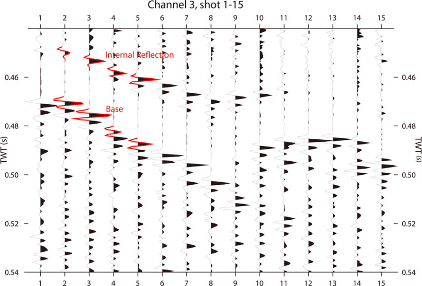
Fig. 8. A close-up of the near-trace gather of the deepest englacial reflector and the bed reflector. The reflection is close to normal incidence. The shape of the source wavelet is marked in red. Note that the amplitudes have been scaled with a 20 ms AGC window to boost the much weaker englacial reflection. At shots 11–15 the englacial reflection is not boosted, as the englacial and the base reflector both fall in the AGC window.
This would cause the basal reflection coefficient, R > 0, because even in the case of lowest possible impedance of frozen base material (frozen till) the numerator of Eqn (1) is positive. As the shape of the wavelet of the base reflection (marked in red in Fig. 8) is similar in shape to the wavelet of the deepest englacial reflection, reflection coefficient R>0. As explained above, we argue that, as a density contrast is very unlikely, this reflection can only be caused by an increase in wave speed that results from a change in COF. We reason that at this depth of ∼40 m above the base, ice mainly deforms through simple shear and, as a result, ice crystals have orientated themselves into a vertical single-maximum fabric. This causes the largest possible compressional wave speed resulting from a COF, as ice crystals have their c-axes parallel to the wave propagation and, thus, a positive reflection coefficient. In addition, the deepest englacial reflector is the strongest reflector observed in the data, so we expect the largest velocity contrast here. This interpretation is consistent with the investigations of wave-speed/depth profiles with non-hyperbolic moveout analysis (Reference Diez, Eisen, Hofstede, Bohlen, Weikusat and KipfstuhlDiez and others, 2012). Without ice-core data or COF modeling data, we can merely assume the state of the COF. Nevertheless, the probable stress regime at this depth, the exceptionally strong reflection and the polarity of the reflection coefficient, are all consistent with our speculative interpretation.
Many authors acknowledge the need to incorporate anisotropy in ice-sheet models (Reference Pettit, Thorsteinsson, Jacobson and WaddingtonPettit and others, 2007; Reference Martín, Gudmundsson, Pritchard and GagliardiniMartín and others, 2009a), but modeling procedures are still in their infancy (e.g. Reference Bargmann, Seddik and GreveBargmann and others, 2012). The development of anisotropy with depth is generally described as smoothly depth-dependent (Reference Martín, Gudmundsson, Pritchard and GagliardiniMartín and others, 2009a) but reflection seismic (Reference Horgan, Anandakrishnan, Alley, Burkett and PetersHorgan and others, 2011), radar studies (Reference Eisen, Hamann, Kipfstuhl, Steinhage and WilhelmsEisen and others, 2007), thin sections (Reference DurandDurand and others, 2007) and borehole sonic logging evidence (Reference BentleyBentley, 1972; Reference DurandDurand and others, 2007; Reference Gusmeroli, Pettit, Kennedy and RitzGusmeroli and others, 2012) suggest that variation in fabric can be abrupt, i.e. over short spatial scales. Such abrupt changes in COF, as indicated by our seismic dataset, could possibly be related to varying impurity contents of the ice, such as dust deposited on the surface during layer deposition. One solution for models to reproduce abrupt changes in COF could be to include an impurity-dependent parameterization for ice viscosity. However, to set up such a parameterization, in situ impurity data from ice cores are required at those locations where double-Raymond bumps observed with radar and englacial seismic layering are found together.
Conclusions
The vibroseis source in combination with a snowstreamer is a fast method for reflection-seismic profiling. The vibroseis method is non-pollutive, in contrast to explosives chemistry, dangerous-goods regulations for transport do not apply, production rate is high and fewer people are involved in the survey. Three people are enough to navigate, shoot, record and travel in an unprepared area. Had the vibrator been an autonomous vehicle, two people could have done the job. High-fold data at increased signal-to-noise ratio can easily be acquired, especially since vibroseis has excellent source control and reproducibility, allowing several sweeps at one location. The signal penetrates well through firn, but because of the limited bandwidth in the present case, the resolution is poorer than signals from explosives. For englacial reflectors, explosives are clearly superior to the vibroseis source used in this survey. To detect the same number of englacial reflectors with the vibroseis source as are detected with the 250 g explosive source, a sweep up to 300 Hz would be needed. Currently, efforts are underway to obtain such data at Kohnen Station, Dronning Maud Land, where the EPICA DML ice core is available to merge seismic observations with in situ physical properties.
We interpret all deeper englacial reflection as caused by changes in the COF. The continuous englacial seismic reflectors at Halvfarryggen ice dome suggest the ice experiences changes in its COF as it develops from top to bottom. These changes in COF should be abrupt, as otherwise they would not cause such considerable reflections in the explosive data. Moreover, they likely occur in layer stacks less than the tuning thickness of the vibroseismic wave (∼13.5m) apart. Our explosive data indicate that changes in COF have a considerable lateral coherent extent over at least two ice thicknesses, as several reflectors are seen along the whole seismic line.
The presence of continuous englacial reflections probably caused by changing COF has implications for flow modeling at ice domes, such as the estimate of ice-core integrity with depth and temporal stationarity. Current ice-dynamic models considering COF anisotropy are only capable of reproducing smooth changes in COF and assume no recrystallization processes (Reference Martín, Gudmundsson, Pritchard and GagliardiniMartín and others, 2009a; Reference Drews, Martín, Steinhage and EisenDrews and others, 2013). Although models are able to reproduce the englacial stratigraphy as recorded with radar, i.e. the distribution of isochrones, they likely fail to reproduce abrupt transitions in COF. By extending the covered offsets of sufficiently high-frequency seismic datasets and improved source systems, as proposed by Reference EisenEisen and others (2010), to increase signal-to-noise ratio and avoid short-period multiples as the ghost, it should be possible to deduce the degree of change in COF across a layer boundary from the associated reflector’s spatial phase signature and non-hyperbolic moveout correction. Together with a denser spatial coverage, such as grids, it moreover seems possible to deduce the spatial distribution of COF across an area of interest, and even apply spatial three-dimensional seismic approaches. This will provide datasets of physical properties which allow data assimilation into ice-dynamic models by constraining not only layer geometry, but also physical properties, such as viscosity prescribed by COF.
Acknowledgements
Initial ideas for this survey were based on discussions with Richard Hindmarsh and Carlos Martín during a research visit to the British Antarctic Survey, funded by the SCAR fellowship scheme 2006-07 and an ‘Emmy Noether’-scholarship EI 672/4-1 of the German Research Foundation (DFG) to O.E. Fieldwork and preparation of this work was supported by the DFG ‘Emmy Noether’-program grant EI 672/5-1 to O.E. UK Natural Environment Research Council (NERC) grant NE/E012914/1 partly supported D.J. We thank Ice Core and Drilling Services (ICDS), PSL and the US Natural Science Foundation for their support in the adaption of the air-pressure drill (RAMdrill) for the Alfred Wegener Institute (AWI). These results would not have been obtained without the continuous support of AWI logistics staff. Special thanks to Sverrir Hilmarson and Rick Blenkner for field assistance, and Reinhard Drews and Niklas Neckel for providing ice-divide and DEM data and tireless help in the field. Alessio Gusmeroli and the second reviewer are thanked for their reviews.


