


1. Introduction
Scale-resolving simulations of flows at industrial scales and high Reynolds numbers  $Re$ can currently not reasonably be performed using wall-resolved large-eddy simulations (wrLES) because of their too high computational cost. Indeed, according to Choi & Moin (Reference Choi and Moin2012), the number of grid points increases as $Re^{13/7}$ for such simulations. Moreover, it was shown by Piomelli & Balaras (Reference Piomelli and Balaras2002) that, for Reynolds numbers above $O(10^6)$, 99 % of the grid points in the mesh are used to resolve the inner layer ( $=$ near-wall region) of the boundary layer which only represents around 10 % to 15 % of its thickness. The grid-point requirements can thus be drastically reduced by modelling the effect of this inner layer on the flow using a so-called wall model. When such a model is used, the number of grid points scales linearly with $Re$, as also shown by Choi & Moin (Reference Choi and Moin2012).
Wall models for large-eddy simulation (LES) rely on the relative decoupling between the inner part of the boundary layer and the rest of the flow. The flow is assumed to follow a universal profile in the near-wall region of the boundary layer whereas the rest of the flow is assumed to be properly captured by the LES. The LES thus still captures a significant part of the boundary layer and is driven by the problem geometry. Three main types of wall models can be distinguished:
(i) Algebraic (or analytical) models where the wall shear stress is directly computed from the LES flow data using the law of the wall for the near-wall region. These models were the first used to perform wall-modelled LES (wmLES) by Deardorff (Reference Deardorff1970) and later by Schumann (Reference Schumann1975). Piomelli et al. (Reference Piomelli, Ferziger, Moin and Kim1989) proposed an improvement of such model by using the velocity a short distance downstream to evaluate the local wall shear stress. In such a framework, Reichardt's formula (Reichardt Reference Reichardt1951) is often used to approximate the law of the wall in a convenient way as it reproduces, in a single formula, the laminar viscous sublayer, the buffer region and the fully turbulent outer region (with the log law); hence allowing us to maintain accuracy when the $y^+$ value of the used LES data falls below the log region.
(ii) Two-layer models, where a separate set of equations is solved within the near-wall part of the boundary layer. The equations solved there are the so-called boundary layer equations, as in Balaras, Benocci & Piomelli (Reference Balaras, Benocci and Piomelli1996), Duprat et al. (Reference Duprat, Balarac, Métais, Congedo and Brugière2011), Kawai & Larsson (Reference Kawai and Larsson2012), Piomelli & Balaras (Reference Piomelli and Balaras2002) and Park & Moin (Reference Park and Moin2014), and which all require an appropriate modelling of the turbulent viscosity profile. Frère et al. (Reference Frère, Hillewaert, Chatelain and Winckelmans2018) studied the balance of the different terms constituting the boundary layer equations using wrLES data of the flow around an airfoil and observed that, for values of
$y^+$ sufficiently large ($\kern 1.5pt y^+\geq 30$), the convective and pressure gradient terms essentially compensate each other. This observation allows us to further simplify the boundary layer equations to only consider the diffusive terms, which can then be integrated on a one-dimensional mesh.Other authors (Chung & Pullin Reference Chung and Pullin2009; Wu & Meyers Reference Wu and Meyers2013) use a specifically modified Subgrid-Scale (SGS) model in the near-wall region (thus relying only on the LES solver but also requiring us to discretize this near-wall region). In Davidson & Peng (Reference Davidson and Peng2003), the near-wall layer is modelled using a turbulent viscosity obtained from the
$k-\omega$ Reynolds-averaged Navier–Stokes (RANS) equations. Even though these approaches solve the same set of equations in the whole domain, they can still be considered as two-layer modelling as the unresolved scales are modelled differently in the near-wall layer and the rest of the domain.(iii) Machine learning and in particular neural networks (NN) were also used by several authors, such as Zhou, He & Yang (Reference Zhou, He and Yang2020) or Boxho et al. (Reference Boxho, Rasquin, Toulorge, Dergham, Winckelmans and Hillewaert2022). Such approaches could possibly allow the development of models for non-equilibrium flows; yet they require the training of NN, hence the need for reference data.


Developments were made to generalize the former two approaches to take compressibility effects into account. For instance, Bocquet, Sagaut & Jouhaud (Reference Bocquet, Sagaut and Jouhaud2012) used a two-layer model in which the compressible boundary layer equations were solved and compared it with a quasi-analytical model based on Reichardt's formula with the temperature, viscosity and density measured at the wall. This was, however, proposed for an isothermal wall and the Kader law (Kader Reference Kader1981) was used to provide the wall heat flux. Even though the proposed quasi-analytical model and the compressible boundary layer model showed similar performance for low Reynolds number supersonic channel flow test cases, the error on the velocity profile was significant.
A similar quasi-analytical wall model was used by Catchirayer et al. (Reference Catchirayer, Boussuge, Sagaut, Montagnac, Papadogiannis and Garnaud2018) for an isothermal wall. They also proposed a model to compute the wall temperature in the case of an adiabatic wall, using a Crocco–Busemann-type relation and the off-wall temperature and velocity data. This wall model was, however, only tested on the adiabatic wall in quasi-incompressible cases, yielding satisfactory results.
The present work proposes to investigate the possibility of using a quasi-analytical wall model where the compressible flow data are scaled before being fed to the wall model. Such scalings have already been proposed to better collapse the compressible simulation data on the universal incompressible laws, the most commonly used being the Van Driest transformation (Van Driest Reference Van Driest1951). However, in the late 1940s, Howarth (Reference Howarth1947) and Stewartson (Reference Stewartson1949) proposed scalings to deduce the results of compressible flows from equivalent incompressible results. To the authors’ knowledge, such scalings have never been investigated to propose a simple wall model for compressible flows.
In this paper, the results of wrLES of adiabatic compressible turbulent channel flows at a friction Reynolds number of  $Re_\tau \simeq 1000$ and at two centreline Mach numbers $M_c$ (one subsonic, one supersonic) are first presented, as they will later be used as reference for the evaluation and validation of our proposed wall model for wmLES. Then, the complete wall-modelling strategy is explained, including the specific tabulated nonlinear solver of Reichardt's formula, the determination of the wall temperature and the investigated scalings to take into account compressibility effects. The results of wmLES of the same compressible turbulent channel flow cases are presented and compared with those of the reference wrLES. The consistency of the new wall model at low Mach numbers is also verified by comparing the results of wmLES at $M_c= 0.25$ with those of reference incompressible direct numerical simulation (DNS) data from Lee & Moser (Reference Lee and Moser2015) at $Re_\tau =1000$ and $5200$. Finally, the proposed wall model is also applied to a turbulent channel flow at $M_c=1.5$ and $Re_\tau =5200$.
2. Wall-resolved simulations of compressible channel flows at $\boldsymbol {Re_\tau \simeq 1000}$

In order to obtain reference data for the wall-model assessment, two wrLES of compressible and turbulent channel flows have been performed. The target Reynolds number was set to  $Re_\tau = 1000$ and two centreline Mach numbers $M_c$ were investigated: (i) a subsonic case at $M_c \simeq 0.76$ and (ii) a supersonic case at $M_c \simeq 1.5$.
2.1. Fluid properties
For all simulations, the fluid is air and is treated as a perfect gas with  $R= 287.1\ {\rm J}\,({\rm kg}\ {\rm K})^{-1}$ and $\gamma =1.4$. The Prandtl number is $Pr = {\mu c_p}/{\kappa } = 0.71$ and the Sutherland law is used for the dynamic viscosity
 \begin{equation} \frac{\mu}{\mu_{ref}} = \left(\frac{T}{T_{ref}}\right)^{3/2} \left(\frac{T_{ ref} + S}{T+S}\right), \end{equation}
with  $\mu _{ref} = 1.716\times 10^{-5}\ {\rm Pa}\ {\rm s}$ at $T_{ref} = 273.15\ {\rm K}$ and $S = 110.4\ {\rm K}$. The specific heat at constant pressure, $c_p$, is considered constant. The thermal conductivity $\kappa$ is determined from the dynamic viscosity and the Prandtl number.
2.2. Simulation set-up
The simulations are performed using the Argo code developed by Cenaero (Hillewaert Reference Hillewaert2013), which uses a discontinuous Galerkin method (DGM). For the wall-resolved simulations, a third-order ( $\,p=3$) polynomial finite element space is used over the whole domain, as this offers a good compromise between accuracy and computational cost. The modified simple low dissipation advection upstream splitting method, proposed by Kitamura & Shima (Reference Kitamura and Shima2010), is used as an approximate Riemann solver at interfaces between elements. For the diffusive terms, a symmetric interior penalty (SIP) method is employed (Arnold et al. Reference Arnold, Brezzi, Cockburn and Marini2002). The time integration is implicit and second order, using the 3-point backward difference formula. The nonlinear system is solved using a Newton/Generalized Minimal Residual (GMRES) method preconditioned with block Jacobi. A reduction in residual of $10^{-4}$ compared with the value of the residual at the beginning of each time step is imposed in order to obtain a good convergence. The solver performs implicit LES (ILES). The ILES approach using DGM/SIP was shown to produce results comparable to those of reference solvers when tested on channel flows at Reynolds numbers up to $Re_\tau \simeq 1000$ by de Wiart et al. (Reference de Wiart, Hillewaert, Bricteux and Winckelmans2015).
Adiabatic walls are considered and the meshes are identical for both cases. The domain size in the three directions is  $L_x \times L_y \times L_z = 2{\rm \pi} h\times 2h\times {\rm \pi}h$ (where h is the channel half-height) and the mesh is composed of $N_x \times N_y\times N_z = 64\times 32\times 64$ structured hexahedra. Since $p=3$ elements are used, this represents $256\times 128 \times 256$ degrees of freedom per equation. The mesh is uniform in the homogeneous directions ( $x$ and $z$) and is stretched in the $y$ direction using
 \begin{equation} \frac{y}{h} = 1+\frac{\tanh\left(\alpha\left(\xi-1\right)\right)}{\tanh\left(\alpha\right)}, \end{equation}
where  $\xi = {2i}/{N_y}$ with $i=0,\ldots,N_y$. The stretching parameter is set to $\alpha =2.6$. The resolution in wall coordinates for both cases is given in table 1. Note that the computation of the resolution is based on the distance between two successive degrees of freedom within an element instead of the usual element length, in order to take into account the higher resolution capability of high-order finite element methods.
Table 1. Resolution in wall coordinates for the wall-resolved simulations at  $Re_\tau \simeq 1000$.

A second simulation was performed in the supersonic regime with a doubling of the elements in the vertical direction to ensure that the proposed mesh allows us to have an accurate reference. This mesh preserves the wall resolution but reduces the stretching, effectively increasing the resolution in the centre of the channel. The results of this simulation are superimposed on those of the base mesh presented previously and are observed to match almost perfectly with the coarser mesh.
The flow statistics are averaged in time over roughly 11 normalized times  $t^+ = h/u_\tau$, and in the homogeneous directions. The time averaging operation is noted $(\tilde{\cdot })$. With that, we define the time-averaged density $\tilde {\rho }$ and pressure $\tilde {p}$. Favre averaging is then applied to the time-averaged velocity $\overline{u}$ and temperature $\overline{T}$, defined as
 \begin{equation} \bar{u} = \frac{\widetilde{\rho u}}{\tilde{\rho}}, \quad \bar{T} = \frac{\widetilde{\rho T}}{\tilde{\rho}}= \frac{\tilde{p}}{R \tilde{\rho}}. \end{equation}
The notation  $\bar {\mu }$ stands for $\mu (\bar {T})$ and the notation ${\bar {\tau }}_w$ stands for the time-averaged wall shear stress. The fluctuating velocity components associated with the Favre averaging are defined as
 \begin{equation} u_i'' = u_i-{\bar{u}}_i . \end{equation}
 The mean pressure gradient imposed in the  $x$ direction is dynamically adapted so as to maintain a constant mass-flow rate. To maintain thermal equilibrium, the power produced by the forcing pressure gradient is omitted in the total internal energy equation.
2.3. Results
The friction Reynolds number, defined as  $Re_\tau =h^+={h\sqrt {\tilde {\rho }_c \bar {\tau }_w}}/{\bar {\mu }_c}$ for a compressible channel flow, was measured as $Re_\tau =1001$ in the subsonic case, with a centreline Mach number of $M_c\simeq 0.76$; while it was measured as $Re_\tau = 955$ in the supersonic case, with $M_c \simeq 1.51$.
Figure 1 shows the velocity profile for both cases: first using the semi-local normalization for both quantities, i.e.
 \begin{equation} \left. \begin{aligned} y^+ & = \frac{\sqrt{\tilde{\rho} {\bar{\tau}}_w}}{\bar{\mu}} y ,\\ \bar{u}^* & = \sqrt{\frac{\tilde{\rho}}{\bar{\tau}_w}} \bar{u} , \end{aligned} \right\} \end{equation}
in figure 1(a); and then using the non-dimensionalization recommended by Huang, Coleman & Bradshaw (Reference Huang, Coleman and Bradshaw1995) which uses the semi-local normalization for  $y$ and the Van Driest transformation (Van Driest Reference Van Driest1951) for $\bar {u}$
 \begin{equation} \bar{u}^+= \sqrt{\frac{\tilde{\rho}_w}{\bar{\tau}_w}}\int_0^{\bar{u}} \sqrt{\frac{\tilde{\rho}}{\tilde{\rho}_w}}\, {\rm d}\bar{u}^{'} , \end{equation}
in figure 1(b).

Figure 1. Velocity profiles in wall coordinates for the cases at  $M_c \simeq 0.76$ (dashed line) and $M_c \simeq 1.51$ at normal (thick solid line) and higher resolutions (dotted line). The incompressible flow DNS data from Lee & Moser (Reference Lee and Moser2015) (thin solid line) and the wrLES data from de Wiart et al. (Reference de Wiart, Hillewaert, Bricteux and Winckelmans2015) at $M_c\simeq 0.10$ (dash-dotted line) are also shown for comparison. (a) Using the semi-local normalization for both quantities. (b) Using the semi-local normalization for $y$ and the Van Driest transformation for $\bar {u}$.
This figure shows that the Van Driest transformation allows us to reduce the Mach number dependence on the normalized velocity profile, while still not perfectly collapsing on the incompressible DNS or wrLES data. This is due to the relatively low Reynolds number and the related large contribution of the viscous sub-layer. Several authors have proposed more advanced transformations to better take the effect of the viscous sub-layer into account, see Huang & Coleman (Reference Huang and Coleman1994), Brun et al. (Reference Brun, Petrovan Boiarciuc, Haberkorn and Comte2008), Zhang et al. (Reference Zhang, Bi, Hussain, Li and She2012), Modesti & Pirozzoli (Reference Modesti and Pirozzoli2016) and Trettel & Larsson (Reference Trettel and Larsson2016).
The velocity profiles are also shown in outer coordinates in figure 2, i.e. non-dimensionalized using the centreline velocity  $\bar {u}_c$ and the channel half-height $h$. The observed behaviour is very similar to that seen in LES of channel flows at lower Reynolds numbers performed by Brun et al. (Reference Brun, Petrovan Boiarciuc, Haberkorn and Comte2008) with a steeper (respectively flatter) velocity profile close to the wall (respectively centreline) with increased Mach number.

Figure 2. Velocity profiles in outer coordinates for the cases at  $M_c \simeq 0.76$ (dashed line) and $M_c \simeq 1.51$ at normal (thick solid line) and higher resolutions(dotted line). The incompressible flow DNS data from Lee & Moser (Reference Lee and Moser2015) are also shown for comparison (thin solid line).
The root-mean-square (r.m.s.) velocity fluctuation profiles are shown in figure 3. These fluctuation profiles are non-dimensionalized using the wall shear stress and the local density. Thus
 \begin{equation} \overline{u''_{i,rms}}^+= \sqrt{\frac{\overline{u''_i u''_i}}{\bar{\tau}_w/\tilde{\rho}}} \quad \text{where} \ \overline{u''_i u''_i} = \frac{\widetilde{\rho u''_i u''_i}}{\tilde{\rho}}. \end{equation}
Figure 3. Velocity fluctuation profiles in wall coordinates for the cases at  $M_c \simeq 0.76$ (dashed line) and $M_c \simeq 1.51$ at normal (thick solid line) and higher resolutions (dotted line). The incompressible flow DNS data from Lee & Moser (Reference Lee and Moser2015) and the wrLES data from de Wiart et al. (Reference de Wiart, Hillewaert, Bricteux and Winckelmans2015) at $M_c\simeq 0.10$ (dash-dotted line) are also shown for comparison (thin solid line). Top: $\overline {u''_{rms}}^+$, middle : $\overline {w''_{rms}}^+$, bottom: $\overline {v''_{rms}}^+$.
The evolution of the near-wall streamwise fluctuation peak with increasing Mach number is similar to what is obtained by Modesti & Pirozzoli (Reference Modesti and Pirozzoli2016) in DNS and using the same normalization. They indeed observed an increase of the streamwise velocity fluctuation  $\overline {u''_{rms}}^+$ peak when increasing the Mach number. For the spanwise and vertical profiles, a slight decrease of fluctuation amplitude is observed when increasing the Mach number. Overall, the dependence in Mach number of the velocity fluctuation profiles is not as significant as for the average velocity profile.
Figure 4 shows the temperature profile, normalized by the total temperature at the centre of the channel
 \begin{equation} \bar{T}_{0,c} = \bar{T}_c\left(1+\frac{\gamma-1}{2}\bar{M}_c^2\right) . \end{equation}
The normalized wall temperature is seen to decrease when the Mach number is increased, which is consistent with the experimental observations of Van Driest (Reference Van Driest1951) for fluids with Prandtl number lower than unity (see also later the modelling of the profile using a recovery factor with (3.3)).

Figure 4. Temperature profiles for the cases at  $M_c \simeq 0.76$ (dashed line) and at $M_c \simeq 1.51$ at normal (thick solid line) and higher resolutions (dotted line).
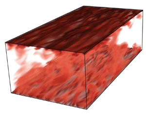
Finally, a volume rendering of the instantaneous normalized temperature field, as well as the instantaneous Mach number fluctuations in a slice of the domain, computed as  $M'' = M-\bar {M}$, are shown in figure 5. We observe that the Mach number fluctuations are significant, with amplitudes up to 0.75.

Figure 5. Instantaneous views of the case at  $M_c\simeq 1.51$. (a) Volume rendering of the temperature field. (b) Mach number fluctuations in a slice.
3. Wall-modelling strategy
The different wall models used to perform the wmLES of the compressible channel flow cases are presented in this section. First, the base wall model, validated for the wmLES of incompressible flows by Frère et al. (Reference Frère, de Wiart, Hillewaert, Chatelain and Winckelmans2017), is introduced. Then, the three scalings for compressible flows are presented and their implementation is detailed. Since these scalings partly rely on unknown wall quantities, the approach used to estimate these quantities is explained and its accuracy assessed on the two compressible channel flow cases.
3.1. Baseline wall model for incompressible flows
The base wall model used in this study relies on the law of the wall for incompressible flows, and fitted using Reichardt's formula
 \begin{equation} \bar{u}_{Reichardt}^+\left(y^+\right) = \frac{1}{\kappa}\log\left(1+\kappa y^+\right) + \left(C-\frac{1}{\kappa}\log\kappa\right)\left(1 - \exp\left(-\frac{y^+}{11}\right)-\frac{y^+}{11}\exp\left(-\frac{y^+}{3}\right)\right) . \end{equation}
We use  ${1}/{\kappa }= 2.61$ and $C=4.25$, in accordance with latest calibrations (see also Winckelmans & Duponcheel Reference Winckelmans and Duponcheel2021). This equation can be solved for $\bar {\tau }_w$ given the averaged values of $\bar {u}_1$ measured at the wall-model injection location $y_1$. Only the component of velocity tangent to the wall is used to compute the wall shear stress. Several authors (Schumann Reference Schumann1975; Piomelli & Balaras Reference Piomelli and Balaras2002; Gillyns, Buckingham & Winckelmans Reference Gillyns, Buckingham and Winckelmans2022) choose to average the velocity in time and/or space. However, as investigated by Lee, Cho & Choi (Reference Lee, Cho and Choi2013) and Frère et al. (Reference Frère, de Wiart, Hillewaert, Chatelain and Winckelmans2017), imposing the value of the wall shear stress instantaneously and locally is sufficient to predict the mean velocity profile. This pointwise and instantaneous approach is also used in the present work, as it can be generalized to transient and non-homogeneous flows. The complete wall-modelling strategy will thus be presented using local and instantaneous quantities.
To solve (3.1), instead of using a Newton–Raphson method, as done by Bocquet et al. (Reference Bocquet, Sagaut and Jouhaud2012), a tabulated approach is used here, as proposed by Maheu, Moureau & Domingo (Reference Maheu, Moureau and Domingo2012). In this version, the value of  $\log (y^+_1 u^+_1) = \log (\kern 1.5pt {y_1 u_1 \rho }/{\mu })$ is computed. The value of $y_1^+$ is then retrieved from pre-calculated tabulated values of $\log (y^+ u^+_{Reichardt})$ stored as a function of $\log (y^+)$. The use of the logarithmic version of the relation is based on the observation that the relation between $\log (y^+ u^+)$ and $\log (y^+)$ is almost linear; hence, an accurate value of $y^+$ can be efficiently computed from the look-up table with only a few tabulated entries and using a linear interpolation between nearby entries. The wall shear stress is finally computed as
 \begin{equation} \tau_w = \frac{1}{\rho}\left(\mu\frac{y^+_1}{y_1}\right)^2. \end{equation}
This wall model was shown to provide accurate results in the framework of DGM/ILES by Frère et al. (Reference Frère, de Wiart, Hillewaert, Chatelain and Winckelmans2017) for high Reynolds number incompressible flows, and it will serve as the baseline model for the present work. It will also be the foundation of the wall models investigated further.
3.2. Scalings for compressible flows
In order to derive a wall model compatible with compressible flows, the flow quantities measured in the simulation must be scaled so as to better follow the law of the wall valid for incompressible flows. The baseline wall model described above is then applied on those scaled quantities to finally obtain the wall shear stress.
Three transformations are studied in this work to achieve the necessary scaling: (i) the Howarth–Stewartson (HS) transformation which maps a compressible boundary layer to an incompressible boundary layer with same mass-flow rate, (ii) a modified Van Driest transformation proposed by Brun et al. (Reference Brun, Petrovan Boiarciuc, Haberkorn and Comte2008) and (iii) a blending of those two scalings.
These transformations rely on the density and temperature variations close to the wall; an estimation of these quantities at the wall is thus necessary. In the following, the quantities related to the transformed flow will be noted with uppercase symbols.
3.2.1. Estimation of thermodynamic quantities at the wall
In order to find an estimation of the wall temperature, Walz's relation (Walz Reference Walz1969) is used
 \begin{equation} T = T_w+\left(T_r-T_w\right)\left(\frac{u}{u_e}\right) + \left(T_e-T_r\right)\left(\frac{u}{u_e}\right)^2, \end{equation}
where
 \begin{equation} T_r = T_e\left( 1 + r\frac{\gamma-1}{2}M_e^2\right), \end{equation}
is the recovery temperature and the index  $e$ denotes the edge of the boundary layer. In this study, the recovery factor $r$ is taken as $r\simeq Pr^{1/3}$, as proposed by Van Driest (Reference Van Driest1951) for a turbulent boundary layer. As this study only deals with adiabatic walls, the recovery to wall temperature ratio is unitary and (3.3) can be simplified to
 \begin{equation} T = T_w - r\frac{\gamma-1}{2}\frac{u^2}{\gamma R}. \end{equation}
 Introducing the quantities measured in the flow at the location where the wall model is injected, noted with subscript ‘ $1$’, (3.5) becomes
 \begin{equation} T_w = T_1 \left(1 + r\frac{\gamma-1}{2}M_1^2\right), \end{equation}
thus providing an estimation of the wall temperature using only the local velocity and temperature at  $y_1$.
We also note that combining (3.6) with (3.5) taken at any location in the boundary layer gives
 \begin{equation} T = T_1\left(1 +r \frac{\gamma-1}{2}M_1^2\right) - r \frac{\gamma-1}{2} \frac{u^2}{\gamma R}, \end{equation}
which makes it possible to compute the temperature at any location in the boundary layer from the velocity data. Using (3.7) with the velocity data from the wrLES of the compressible turbulent channel flows and comparing the result with the actual temperature data of the wrLES, as done in figure 6, shows that this simplified model accurately approximates the real temperature profile in the compressible cases.

Figure 6. Comparison between the temperature profile measured in the wrLES (lines) and the modelled temperature profile (symbols) for the cases  $M_c\simeq 0.76$ and $M_c\simeq 1.51$.
The injection location of the wall model will here be taken at  $y/h \simeq 0.14$, which is a typical first cell height for wmLES of a turbulent channel flow. The error on the $T_w$ prediction is then 0.05 % and 0.11 % for the subsonic and supersonic cases, respectively.
Finally, to fully characterize the thermodynamical state at the wall, the pressure is considered constant across the first element. Thus
 \begin{align} p_w &= p_1 , \end{align}
 \begin{align} \Rightarrow \quad \rho_w &= \frac{p_1}{R T_w} . \end{align}
3.2.2. Howarth–Stewartson transformation
This transformation requires the definition of a reference state to which the initial compressible flow is mapped; in our case, an incompressible flow with constant density  $\rho _w$ and constant viscosity $\mu _w = \mu (T_w)$.
The wall-normal coordinate of the scaled flow is then defined as
 \begin{equation} {Y}_1 = \int_0^{y_1} \left(\frac{\rho}{\rho_w}\right)\,{{\rm d} y}. \end{equation}
A compressible streamfunction  $\psi$ is introduced so that $\rho u = \rho _w({\partial \psi }/{\partial y})$ and $\rho v =-\rho _w({\partial \psi }/{\partial x})$. To ensure conservation of mass-flow rate between physical and transformed flow, this compressible streamfunction must have the same value as its scaled incompressible counterpart ${\hat {\psi }}({X},{Y})$. This condition results in a unitary scaling for the velocity
 \begin{equation} {U}_1 = u_1. \end{equation}
 The baseline model, described in § 3.1 is then applied on the transformed  ${Y}_1$ and ${U}_1$, along with the fluid properties of the transformed flow ( $\rho _w$ and $\mu _w$), providing the wall shear stress $\tau _w$. However, the integral in (3.10) cannot be computed explicitly as the density profile is not known below the first grid point. An iterative approach, using Walz's relation (Reference Walz1969) and the velocity profile given by the Reichardt formula could be implemented. However, this method was found in a priori testing to yield a value for $Y_1$ only around 0.5 % different from that provided when using a simple explicit trapezoidal integration method; the latter was thus implemented to perform the $y$-coordinate scaling.
3.2.3. Modified Van Driest scaling
The Van Driest (VD) transformation was used in previous sections to scale the velocity so as to better fit the near-wall incompressible flow velocity profile in wall coordinates. This transformation consists of a scaling of the velocity derivative
 \begin{equation} \frac{{\rm d}{U}}{{\rm d}u} = \sqrt{\frac{\rho}{\rho_w}}. \end{equation}
Brun et al. (Reference Brun, Petrovan Boiarciuc, Haberkorn and Comte2008) proposed an improved scaling that also acts on the derivative of the  $y$ coordinate. The complete transformation is
 $$\begin{gather} {Y} = \int_0^y \frac{\mu_w}{\mu}\,{{\rm d} y}, \end{gather}$$
 $$\begin{gather}{U} = \int_0^u \frac{y}{{Y}}\frac{\mu_w}{\mu}\sqrt{\frac{\rho}{\rho_w}}\,{\rm d}u. \end{gather}$$
It was pointed out by Brun et al. (Reference Brun, Petrovan Boiarciuc, Haberkorn and Comte2008) that applying this transformation on the velocity profile decreases the spread of the value of the  $C$ coefficient in the log region for different flow configurations, yet does not cancel it entirely.
In the present work, the  $y$-coordinate transformation is approximated, at the first grid point, using
 \begin{equation} {Y}_1 = \frac{\mu_w}{\mu_1}y_1, \end{equation}
as this yields better results when used in the complete wall model than using a trapezoidal rule. Equation (3.14) is then simplified to the expression of the classical VD transformation and can be integrated analytically, recalling that the pressure is uniform near the wall and that the temperature follows Walz's relation (Walz Reference Walz1969)
 \begin{align} {U}_1 &=\int_0^{u_1}\sqrt{\frac{T_w}{T}}\,{\rm d}u, \end{align}
 \begin{align} &= \int_0^{u_1}\left(1-\frac{r}{2\,c_p\,T_w}u^2\right)^{-1/2}\,{\rm d}u, \end{align}
 \begin{align} &= \sqrt{\frac{2c_p T_w}{r}}\arcsin\left(\sqrt{\frac{r}{2c_p T_w}} u_1\right). \end{align}
A difference of at most 1 % is observed on the input value of the baseline wall model (i.e.  ${{U}_1{Y}_1 \rho _w}/{\mu _w}$) between the result provided by the numerical integration of (3.13) and (3.14) using the wrLES data, and the value obtained using (3.15) and (3.18).
3.2.4. Present scaling
The third proposed scaling can be seen as a blending of the two previous ones. As for the HS scaling, it relies on a scaling of the  $y$-coordinate and the conservation of mass-flow rate between the initial and transformed flows. However, the $y$-coordinate transformation contains now a factor to take the viscosity variation into account
 $$\begin{gather} {Y}_1 = \int_0^{y_1}\frac{\mu_w}{\sqrt{\rho_w}}\frac{\sqrt{\rho}}{\mu}\,{{\rm d} y}, \end{gather}$$
 $$\begin{gather}{U}_1 = \sqrt{\frac{\rho_1}{\rho_w}}\frac{\mu_1}{\mu_w} u_1 . \end{gather}$$
The  $({\mu _w}/{\sqrt {\rho _w}})({\sqrt {\rho }}/{\mu })$ scaling factor for $y$ is inspired by the recommendation of Trettel & Larsson (Reference Trettel and Larsson2016).
As was the case when using the HS transformation, the integral for  ${Y}_1$ is evaluated using a trapezoidal rule, providing a simple explicit scaling. When comparing the numerical integration of (3.19) using wrLES data with the trapezoidal rule, the error done on ${Y}_1$ is lower than 2 % for both Mach numbers as long as $y_1/h \lesssim 0.15-0.20$, which is a necessary condition to use such wall model solely based on the law of the wall.
Other scalings exist to collapse compressible flow results to equivalent incompressible flow results, such as those proposed by Volpiani et al. (Reference Volpiani, Iyer, Pirozzoli and Larsson2020), Trettel & Larsson (Reference Trettel and Larsson2016) and Griffin, Fu & Moin (Reference Griffin, Fu and Moin2021). These more recent scalings proved to collapse more accurately the compressible flow data onto incompressible results in the post-processing phase. However, the latter two rely on using derivatives of the time-averaged flow quantities in the wall-normal direction. Using such derivatives, evaluated locally and instantaneously in the simulation, would be prone to large errors, and also in the under-resolved first off-wall elements; hence introducing large deviations in the model. The scaling proposed by Volpiani et al. (Reference Volpiani, Iyer, Pirozzoli and Larsson2020) is also similar to the modified VD transformation Brun et al. (Reference Brun, Petrovan Boiarciuc, Haberkorn and Comte2008) but the integral present in the velocity scaling cannot be evaluated analytically, which then also introduces large errors when evaluated using the trapezoidal rule. The a priori error was nevertheless computed for this scaling as well, and is shown in figure 8.
3.3. A priori error estimation
Based on the results of the wrLES at  $Re_\tau \simeq 1000$ and at the two centreline Mach numbers, the error on the wall shear stress prediction can be evaluated a priori. To do so, the wall-modelling workflow is followed, taking as input the flow quantities all along the wrLES profiles. The complete workflow, including the baseline wall model, is summarized in figure 7. Note that, in the case where no scaling is used, the centre dotted box is bypassed and thus ${Y}_1=y_1$ and ${U}_1=u_1$.

Figure 7. Wall-modelling workflow.
Applying this methodology to the wrLES data, we obtain the results shown in figure 8 for the error on  $\tau _w$ when using the different wall models compared with the actual wrLES wall shear stress. This figure shows the range between $y^+ = 100$ and $250$, although the present wall model should not be used above $\simeq 200$ for such wmLES at $Re_\tau \simeq 1000$, as the contribution of the complement function that adds to the law of the wall becomes important.

Figure 8. Error on the wall shear stress in per cent when using the wall models on the wrLES data compared with the wrLES wall shear stress; (a)  $M_c \simeq 0.76$, (b) $M_c \simeq 1.51$.
This figure clearly demonstrates how the scaling procedure improves the results concerning the estimation of the wall shear stress that will be further applied via the wall model. In both cases, the use of a scaling decreases the error on  $\tau _w$. At $y^+=150$, which would be a reasonable first cell height for wmLES at $Re_\tau \simeq 1000$, the error when going from $M_c\simeq 0.76$ to $M_c \simeq 1.51$ goes from 14.3 % to 38.5 % when no scaling is applied, and from 12.4 % to 30 % when the VD scaling is used. At the same location, the error only increases from 9.3 % to 17 % when the HS scaling is used, and from 6.2 % to 6.5 % when the present scaling is used. The present scaling thus performs best. We also note that its error remains at the same level when increasing the Mach number.
4. Wall-modelled simulations of compressible channel flows at $\boldsymbol {Re_\tau \simeq 1000}$

This section presents the results of the wmLES of compressible turbulent channel flows at  $Re_\tau \simeq 1000$ and at $M_c\simeq 0.76$ and $M_c\simeq 1.51$ using the baseline wall model and the three scaled versions. Moreover, the wmLES of a channel flow at $M_c\simeq 0.25$ is also performed, thus a quasi-incompressible case. The mean velocity, temperature and density profiles are shown, as well as the velocity fluctuation profiles. Then, the error on the mass-flow rate compared with the wrLES is computed for the different wall models and analysed for increasing Mach numbers.
4.1. Simulation set-up
The computational domain size for the wall-modelled simulations is the same as that for the wall-resolved simulations. The order of the interpolation polynomials is set to 3 in the bulk of the domain and is increased to 4 in the first wall-adjacent elements as this was observed to give the best results in the framework of wall-modelled ILES/DGM by Frère et al. (Reference Frère, de Wiart, Hillewaert, Chatelain and Winckelmans2017) using the same code. For the wall-modelled simulations, the number of elements in the three directions is  $N_x\times N_y\times N_z = 26\times (11p3+2p4)\times 13$. The same stretching function is used (see (2.2)) and the stretching parameter is set to $\alpha =0.4$.
Still following the recommendations of Frère et al. (Reference Frère, de Wiart, Hillewaert, Chatelain and Winckelmans2017), the computation of the wall shear stress through the wall model is based on the flow quantities measured at the bottom degree of freedom of the second wall-adjacent element. The mesh is shown in figure 9 with the degrees of freedom at which the wall model is evaluated shown using a star. There is thus one discontinuous Galerkin (DG) element (with five degrees of freedom) between the wall and the location (bottom of the second DG element) where the flow quantities are measured to evaluate the wall shear stress, allowing us to have an accurate measurement of the flow quantities in the LES, as was also shown by Frère et al. (Reference Frère, de Wiart, Hillewaert, Chatelain and Winckelmans2017) and as was also recommended by Kawai & Larsson (Reference Kawai and Larsson2012). The resolution in wall coordinates for the wmLES, rounded to 5, is given in table 2. Note that, in this case, the resolution in the  $x$ and $z$ directions corresponds to the distance between 2 successive degrees of freedom, whereas $y_1^+$ is the height of the first element.

Figure 9. Mesh used for the wall-modelled simulations. (a) Whole domain and (b) zoom on the near-wall region. The degrees of freedom are shown in grey in the buffer element ( $\kern 1.5pt p=4$) and in black in the bulk elements ( $\kern 1.5pt p=3$). The stars represent the degrees of freedom where the quantities are measured to compute the wall shear stress using the wall model.
Table 2. Resolution in wall coordinates for the wall-modelled simulations at  $Re_\tau \simeq 1000$, rounded to 5. The resolution in the $x$ and $z$ directions corresponds to the distance between 2 successive degrees of freedom, whereas $y_1^+$ is the height of the first element.

Contrary to the wrLES, these wall-modelled simulations are driven using a constant imposed streamwise pressure gradient. The use of this forcing source term was preferred as it does not require information from the first wall-adjacent cell to be determined. This forcing source term is computed using the incompressible DNS results to reach  $Re_\tau = 1000$ for the case at $M_c\simeq 0.25$. For the higher Mach number cases, it is taken as the time-averaged pressure gradient of the wrLES. The wall shear stress of each wmLES will thus be essentially equal to that of the corresponding wrLES, and the error will be evaluated on the mass-flow rate.
4.2. Results
The velocity profiles in wall coordinates are shown in figure 10 for the quasi-incompressible simulations and are compared with the incompressible DNS results of Lee & Moser (Reference Lee and Moser2015) at the same Reynolds number. Moreover, the quasi-incompressible wall-resolved ILES data obtained using DGM/SIP at  $Re_\tau =950$ and $M_c\simeq 0.10$ and presented by de Wiart et al. (Reference de Wiart, Hillewaert, Bricteux and Winckelmans2015) are also shown for a full comparison over the whole range of resolutions of scale-resolving simulations. The wmLES profiles of the compressible channel flows are shown in figure 11 and are compared with the wrLES profiles presented in § 2.

Figure 10. Velocity profiles in wall coordinates for the channel flows at low Mach numbers: reference incompressible flow DNS (Lee & Moser Reference Lee and Moser2015, solid black), wrLES at  $M_c \simeq 0.10$ (de Wiart et al. Reference de Wiart, Hillewaert, Bricteux and Winckelmans2015, dotted black), wmLES at $M_c \simeq 0.25$ without scaling (blue) and with present scaling (red). The vertical dashed black lines show the element boundaries (for readability reasons, those are only shown for the profile obtained using the present scaling).

Figure 11. Velocity profiles in wall coordinates for the channel flows at (a)  $M_c\simeq 0.76$ and (b) $M_c\simeq 1.51$. The vertical dashed black lines show the element boundaries (for readability reasons, those are only shown for the profile obtained using the present scaling).
The semi-local normalization, defined in (2.5), is used for the wall distance and velocity in figures 10 and 11 because, with the solution computed in the first wall-adjacent element being non-physical, the integral present in the classical VD transformation (see (2.6)) cannot be performed with sufficient precision.
Computation element boundaries are shown by vertical dashed lines. There are no degrees of freedom on the channel centreline as it cuts the centre  $p3$ element in two. The degrees of freedom in the first off-wall element will be omitted in all the following graphs as they do not bring any meaningful information. The first degree of freedom shown in those graphs is thus where the flow quantities are evaluated for the calculation of the wall shear stress.
As expected, the proposed wall model yields virtually identical results to the baseline incompressible wall model at low Mach numbers, see figure 10. The obtained velocity profile is also found to be very close to that of the reference incompressible flow DNS.
It can be seen in figure 11 that the error on the velocity profile follows the trends obtained in the a priori error analysis (§ 3.3). Indeed, the velocity profiles obtained with the unscaled wall model exhibit the largest error in both cases, its magnitude increasing with Mach number. The HS and modified VD scalings yield very similar results at subsonic speeds but the accuracy of the former decreases less than that of the latter when going to the supersonic case. Lastly, the presently proposed scaling produces the most accurate velocity profile in both cases, with a significant error reduction for increasing Mach number.
The same velocity profiles are shown in outer coordinates in figure 12. In this figure, the velocity is normalized by the centreline velocity of the wrLES  $u_{c,wr}$ as this better highlights the error on the velocity profile for the different scalings. This figure shows the same trends as what was observed in wall coordinates, the unscaled wall model underevaluating the centreline velocity by 6 % in the subsonic case and by 14 % in the supersonic case, whereas the proposed scaling maintains this error below 2 % in both cases. The error when using the other two scalings lies between these boundaries. A similar behaviour can be observed on the temperature profile in figure 13.

Figure 12. Velocity profiles in outer coordinates for the channel flows at (a)  $M_c\simeq 0.76$ and (b) $M_c\simeq 1.51$. The vertical dashed black lines show the element boundaries.

Figure 13. Temperature profiles for the channel flows at (a)  $M_c\simeq 0.76$ and (b) $M_c\simeq 1.51$.
The density profiles are shown in figure 14. At the lower Mach number, the three scaled wall models, as well as the baseline wall model, produce essentially the same results, accurately retrieving the density variation of the wrLES. When the Mach number is increased to  $M_c \simeq 1.51$, a more significant difference is observed between these models, and the HS and present scalings provide the best overall results.

Figure 14. Density profiles for the channel flows at (a)  $M_c\simeq 0.76$ and (b) $M_c\simeq 1.51$.
The differences in velocity and density profiles yield differences in the computed mass-flow rate for each of the scalings and the error on this global quantity compared with the reference simulation (DNS for the quasi-incompressible case at  $M_c\simeq 0.25$ and wrLES for the cases at $M_c\simeq 0.76$ and $M_c\simeq 1.51$) is summarized in table 3 for all studied cases. Two mass-flow rates are computed: (i) the total mass-flow rate in the channel, including the under-resolved buffer element, noted $Q_m$ and (ii) the mass-flow rate in the resolved part of the channel in the wmLES (i.e. excluding the region covered by the under-resolved buffer element) and noted $Q_m^{res}$. The use of this second diagnostic makes it possible to better appreciate how the unphysical data of the buffer element impact the evaluation of the total mass-flow rate.
Table 3. Error on the total mass-flow rate  $Q_m$ and on the mass-flow rate in the resolved part of the wmLES $Q_m^{res}$, at $M_c \simeq 0.25$, $M_c \simeq 0.76$ and $M_c \simeq 1.51$.

As expected from the profiles previously shown, the scaled and unscaled wall models have a similar accuracy in terms of mass-flow rate at low Mach number. For the higher Mach numbers, the present scaling provides the best results while all the scaled wall models perform better than the unscaled wall model. For all the considered wall models, the error on the resolved mass-flow rate is slightly lower than the error on the total mass-flow rate but this is not significant. The increase of centreline Mach number from  $M_c\simeq 0.76$ to $M_c\simeq 1.51$ has the effect of increasing the error on the mass-flow rate by more than a factor two for the unscaled wall model and the wall model scaled using the modified VD scaling. For the HS scaling, a slightly lower, yet very high 50 % increase in error is observed. For the present scaling, the evolution of the error on mass-flow rate is non-monotonic: it first increases when increasing the Mach number from $M_c\simeq 0.25$ to $M_c \simeq 0.76$; then a slight decrease in error is observed when going to the supersonic range. This decrease is, however, marginal. When using the ‘resolved’ mass-flow rate, it is even less significant. Concerning the increased error for the wmLES at $M_c\simeq 0.76$ with respect to the wmLES at $M_c\simeq 0.25$, it can also be partially attributed to the fact that the reference used in the low subsonic case is an incompressible flow DNS, whereas that used for the high subsonic case is our compressible flow wrLES.
Globally, the proposed scaling clearly provides improved performances on the prediction of the local quantities (velocity and temperature profiles) and of the global mass-flow rate, both for high subsonic flows and for supersonic flows (at least up the Mach number of 1.5 so far investigated).
The velocity fluctuation profiles are shown in figures 15 and 16. For all cases, the variations in results depending on the used scaling are much less significant than those obtained for the mean velocity profiles. For the low subsonic case in figure 15, both wmLES retrieve well the reference DNS profiles for the vertical and spanwise directions. In the streamwise direction, the fluctuation amplitude is underestimated in the wmLES. However, the obtained profile compares well with that of a wrLES at similar  $Re_\tau$ and $M_c\simeq 0.10$. The underestimation of the fluctuation amplitude is thus inherent to the LES framework.

Figure 15. Fluctuation profiles for the channel flows at low Mach numbers: reference incompressible flow DNS (Lee & Moser Reference Lee and Moser2015, solid black), wrLES at  $M_c\simeq 0.10$ (de Wiart et al. Reference de Wiart, Hillewaert, Bricteux and Winckelmans2015, dotted black), wmLES at $M_c\simeq 0.25$ without scaling (blue) and with present scaling (red).

Figure 16. Fluctuation profiles for the channel flows at (a)  $M_c\simeq 0.76$ and (b) $M_c\simeq 1.51$.
For the high subsonic and supersonic cases in figure 16, the same accuracy is obtained in the transverse directions. In the longitudinal direction, the present scaling provides slightly better results in the region close to the channel centre in the subsonic case, and results similar to those of the other models in the lower part. In the supersonic case, the wmLES profiles are similar and they follow well the wrLES profile.
5. Wall-modelled simulations of compressible channel flows at $\boldsymbol {Re_\tau \simeq 5200}$

In order to investigate the behaviour of the proposed wall model in more practical cases where the inner and outer regions of the boundary layer are well separated, two cases at  $Re_\tau \simeq 5200$ are studied with the wmLES. In a first case, an adiabatic channel flow with $M_c \simeq 0.24$ is computed. The results can thus be compared with the incompressible DNS database of Lee & Moser (Reference Lee and Moser2015) at the same Reynolds number. The second case is a supersonic channel flow with centreline Mach number $M_c \simeq 1.46$. No reference data are available for this Mach number at such high Reynolds number; the computational cost of a wrLES would be too high and is beyond the scope of this study. The results obtained for this case are thus analysed in a more qualitative manner.
5.1. Simulation set-up
The simulation set-up is similar to that of the wmLES at  $Re_\tau \simeq 1000$ (see § 4.1): the domain dimensions, the number of elements and their interpolation orders are the same. Maintaining the number of elements constant when increasing the Reynolds number by a factor of five might seem in contradiction with the requirements of Choi & Moin (Reference Choi and Moin2012). However, the proposed mesh resolution is the same as that used by Frère et al. (Reference Frère, de Wiart, Hillewaert, Chatelain and Winckelmans2017) for a channel flow at the same Reynolds number (and even for a case at $Re_\tau = 50\,000$), and was shown to give good results in the frame of an ILES/DGM. The only change in the mesh compared with that used for the channel flows at $Re_\tau \simeq 1000$ concerns the stretching in the vertical direction, which has been removed here, hence exactly matching the mesh from Frère et al. (Reference Frère, de Wiart, Hillewaert, Chatelain and Winckelmans2017) with the same interpolation orders. This mesh gives a theoretical wall-model injection location of $y^+_1 \simeq 800$ or $y_1/h = 0.154$, which lies at the end of the log layer (as also measured by Winckelmans & Duponcheel Reference Winckelmans and Duponcheel2021), thus within the range of validity of the law of the wall.
The other solver parameters are the same as previously. The Reynolds number is enforced by imposing a constant pressure gradient in the streamwise direction. The friction Reynolds number obtained for the low Mach number simulation ( $M_c \simeq 0.24$) is $Re_\tau =5178$ whereas the supersonic channel reached $M_c \simeq 1.46$ and $Re_\tau = 5166$. The wall resolution is $\Delta y_1^+ = 790$ and $700$ for the subsonic and supersonic cases, respectively.
5.2. Results
5.2.1. Low subsonic channel flow
The obtained mean velocity profile is shown in figure 17 in both wall and outer coordinates. A slight over-prediction of the velocity over the whole channel span is observed. This does not exceed 1 %, which also corresponds to the actual density variation across the channel. Thus, the observed deviation can be attributed to the rather small compressibility effects when increasing the Mach number, resulting in an upwards shift in the velocity profile, as was also observed in figure 1.

Figure 17. Velocity profiles for the channel flow at low Mach number: wmLES at  $M_c \simeq 0.24$ with present scaling (red) and incompressible flow DNS (Lee & Moser Reference Lee and Moser2015, solid black). (a) In wall coordinates. (b) In outer coordinates.
Concerning the fluctuations, shown in figure 18, the wmLES underestimates the longitudinal velocity fluctuations compared with the DNS, as usual for LES simulations. The fluctuation profiles in the  $y$ and $z$ directions are well represented by the wmLES.

Figure 18. Velocity fluctuation profiles for the channel flow at low Mach number and high Reynolds number: wmLES at  $M_c \simeq 0.24$ with present scaling (red) and incompressible flow DNS (Lee & Moser Reference Lee and Moser2015, solid black).
5.2.2. Supersonic channel flow
The obtained mean velocity profile for the supersonic channel at high Reynolds number is shown in figure 19 in both wall and outer coordinates. Given the lack of reference to assess the validity of the results for this case, the wrLES results at  $Re_\tau \simeq 1000$ and $M_c \simeq 1.51$, as well as the incompressible flow DNS data from Lee & Moser (Reference Lee and Moser2015) at $Re_\tau \simeq 5200$, are used as a basis for comparison.

Figure 19. Velocity profiles for the wmLES of supersonic channel flow at high Reynolds number using the present scaling (red). The profiles of the wrLES at similar Mach number and  $Re_\tau \simeq 1000$ (solid black) and of the incompressible flow DNS at $Re_\tau \simeq 5200$ (Lee & Moser Reference Lee and Moser2015, dotted black) are provided for comparison. (a) In wall coordinates. (b) In outer coordinates.
Figure 19(a) shows a significant upward shift of the velocity profile in wall coordinates when compared with the incompressible flow at the same Reynolds number. This shift is physical and is essentially due to the high Mach number; it is indeed seen to be very similar to that observed at  $Re_\tau \simeq 1000$ in figure 1(a). In outer coordinates, the previously observed lower slope near the centre of the channel with an increase of the Mach number is also physical; it is clearly visible when comparing with the incompressible flow profile. The profiles at $Re_\tau \simeq 5200$ and $Re_\tau \simeq 1000$ almost overlap. This very low dependency on the Reynolds number for the bulk velocity profile can also be observed in the DNS results of Yao & Hussain (Reference Yao and Hussain2020) for cooled channel flows at the same Mach number and at increasing Reynolds numbers ( $Re_\tau = 145\unicode{x2013} 1266$). The above elements allow us to have some confidence in the quality of the velocity profiles obtained in our wmLES using the present scaling for supersonic flows at high Reynolds number.
The obtained fluctuation profiles are shown in figure 20. It was observed (figure 3) for wrLES that the spanwise and vertical fluctuations were not strongly dependent on the Mach number. The deviation observed between the incompressible flow and the supersonic channel flows at similar Reynolds numbers should thus exhibit a similar behaviour; it is indeed the case with the usual slight underestimation by the wmLES (attributed to the intrinsic under-prediction of the fluctuations by a LES compared with a DNS). This shift was also observed in the wrLES results. Moreover, the velocity fluctuations in these transverse directions for the wmLES are slightly increased compared with the wrLES at similar Mach number and  $Re_\tau \simeq 1000$. This evolution with increasing Reynolds number is also observed in reference incompressible flow DNS data (see for instance Lee & Moser Reference Lee and Moser2015). The above observations strengthen our confidence in the spanwise and vertical velocity fluctuations obtained by our wmLES.

Figure 20. Velocity fluctuation profiles for the wmLES of supersonic channel flow at high Reynolds number using the present scaling (red). The profiles of the wrLES at similar Mach number and  $Re_\tau \simeq 1000$ (solid black) and of the incompressible flow DNS at $Re_\tau \simeq 5200$ (Lee & Moser Reference Lee and Moser2015, dotted black) are provided for comparison.
In the streamwise direction, the obtained wmLES profile is similar to that of the wrLES profile at similar Mach number and  $Re_\tau \simeq 1000$. As expected, they both stand above the profile for incompressible flow.
Finally, figure 21 shows the obtained density and temperature profiles for this wmLES. These profiles can only be compared with those obtained in the wrLES at similar Mach number and  $Re_\tau \simeq 1000$. As no values are computed at the wall, the profiles were here non-dimensionalized using the channel centreline values. This figure shows, for both quantities, a slightly flatter profile for the wmLES compared with that of the wrLES at a lower Reynolds number. This is expected when increasing the Reynolds number as the near-wall variations will be larger, giving some confidence in the temperature and density profiles obtained in our wmLES.

Figure 21. Density (a) and temperature (b) profiles for the wmLES of supersonic channel flow at high Reynolds number using the present scaling (red). The profiles of the wrLES at similar Mach number and  $Re_\tau \simeq 1000$ are provided for comparison.
6. Conclusions and perspectives
In this study, different scalings were recalled that are used to map the mean profiles of compressible flow into their equivalent incompressible flow. They were simplified with the objective to design a simple quasi-analytical wall model for wmLESof highly compressible flows, and still using the Reichardt formula for the law of the wall in incompressible flows. In this work, an additional scaling was proposed, originating from the combination of the existing ones. The accuracy of the obtained wall models was evaluated on three cases of turbulent channel flow at  $Re_\tau \simeq 1000$: a low Mach number subsonic case (thus directly comparable to an incompressible flow), a high Machnumber subsonic case and finally a supersonic case. For each case, a wrLES was also performed to serve as reference.
The comparison of the wmLES with their wrLES counterparts showed that the proposed hybrid wall model accurately replicates the wrLES profiles in terms of velocity as well as temperature and density. For the velocity fluctuations, no significant differences were observed between the wall models and they all satisfactorily reproduced the wrLES profiles. The error on the mass-flow rate in the channel was used as global metric to compare the wall models and it was shown that the model based on the proposed new scaling achieved a consistent error of approximately 2 % for both the high subsonic and the supersonic cases, whereas the other scalings produced an increase in the error (by a factor of  $1.5$ to $2$). As expected, the unscaled wall model yielded consistently the worst results. In the low subsonic regime, using the proposed new scaled version also led to smaller deviations from the reference wrLES data than when using the unscaled version.
The proposed wall model was then further investigated on a channel flow at high Reynolds number of  $Re_\tau \simeq 5200$: for the low subsonic and the supersonic regimes. The low subsonic wmLES correctly predicts the reference incompressible DNS data, with a deviation on the mass-flow rate of only 0.3 % (also attributed in part to the small compressibility effects). For the supersonic case, the velocity profile was shown to be aligned with its lower Reynolds number counterpart at identical Mach number, which corresponds to the expectations. In terms of fluctuations, both cases gave expected results (in comparison with wrLES at lower Reynolds number and with incompressible DNS at similar Reynolds number). However, the lack of a reference for a supersonic channel at high Reynolds number makes it difficult to provide here a more quantitative analysis of the wmLES performance.
The wall model developed here will be used to perform wmLES of supersonic ejectors where the Mach numbers and the Reynolds numbers are comparable to those investigated here. The results of these simulations will complement the results and observations of previous experimental studies and RANS simulations (Lamberts, Chatelain & Bartosiewicz Reference Lamberts, Chatelain and Bartosiewicz2017; Lamberts et al. Reference Lamberts, Chatelain, Bourgeois and Bartosiewicz2018).
The accuracy of the wall model for flows at Mach numbers higher than  $M_c \simeq 1.5$ should also be further evaluated. Furthermore, this study only focused on a scaling valid for flows with adiabatic walls. Its extension to flows with other boundary conditions will also have to be investigated.
Acknowledgements
Computational resources have been provided by the Consortium des Équipements de Calcul Intensif (CÉCI), funded by the Fonds de la Recherche Scientifique de Belgique (F.R.S.-FNRS) under Grant No. 2.5020.11 and by the Walloon Region. The present research benefited from computational resources made available on the Tier-1 supercomputer of the Fédération Wallonie-Bruxelles, infrastructure funded by the Walloon Region under the grant agreement n $^{\circ }$1117545.
Funding
This research received no specific grant from any funding agency, commercial or not-for-profit sectors.
Declaration of interests
The authors report no conflict of interest.


