


The failure of individual financial institutions is often associated with poor macroeconomic conditions and financial instability. Conventional explanations for failure include liquidity shocks due to the maturity mismatch of assets and liabilities (e.g., the model of Diamond and Dybvig Reference Diamond and Dybvig1983) or insolvency due to impaired assets. Yet both of these explanations are limited in incorporating the institutional details of how financial institutions structure their liabilities. For instance, commercial banks can vary the deposit rate or restrict access to liquidity via withdrawal limitations. Relying on low-cost funding may attract depositors that are ex-ante more susceptible to liquidity shocks—in other words, more “flighty.” What appears across banks as surprise liquidity shocks is actually a function of their predetermined structures. Financial distress can therefore be endogenous to the characteristics of depositors.
In this paper, I study the role of depositor flightiness using building and loan associations (B&Ls) in California during the Great Depression. B&Ls were lending institutions that specialized in loans against real estate, accounting for about one-third of the institutional residential mortgage market at their peak in the 1920s. During the Great Depression, there were a large number of closures via liquidation (both voluntary and involuntary) among B&Ls across the United States. Snowden (2003) attributes the decline of B&Ls to the combination of macroeconomic forces and B&Ls’ unique operating structure.
While B&Ls specialized in mortgage lending throughout their history, they continually innovated on the liability side of their balance sheet. The two dominant plans during the late 1800s and early 1900s were the serial and permanent plans.Footnote 1 In California, these B&L plans issued withdrawable shares, a form of equity contract. Withdrawable shares were frequently structured into series, a form of forced savings plan for new members.Footnote 2 In addition, withdrawable shares featured penalties that made it difficult for members to access funds on short notice.
By the early 1900s, California B&Ls began to adopt the Dayton plan (named after the city in Ohio, where it originated), which eliminated series and removed many aspects of the savings plan and withdrawal penalties. In California, instead of only withdrawable shares, Dayton plans frequently issued investment certificates, a form of debt contract. Investment certificates differed from withdrawable shares because withdrawal penalties were lower, so members could more easily access the full value of their funds, and there was a less rigid savings program. Investment certificates were comparable with certificates of deposit at commercial banks, albeit with a few additional restrictions common to B&Ls (Clark and Chase Reference Clark and Chase1927).
The simultaneous existence of Dayton plans, which emphasized low-cost savings, and non-Dayton plans, which emphasized regular savings and higher withdrawal penalties, represents the key source of liability heterogeneity studied in this paper. Due to the gradual nature of B&L innovation, in some states there were periods of overlap during which there existed non-Dayton plans that looked more like “traditional” B&Ls and newer Dayton plans that were closer in spirit to commercial banks. This paper studies the state of California during the Great Depression, which was one of the states and time periods with the most overlap. I leverage variation across these two types of plans to understand whether member flightiness led to different rates of closure during the Great Depression.
B&Ls in the Great Depression offer an exceptional laboratory to study the effect of flightiness on financial distress. First, the proliferation over the past few decades of different types of derivatives and investments has complicated both sides of financial balance sheets, making it difficult to disentangle the relative effects of specific liabilities. B&Ls at this time had very simple liability structures that allow me to focus on the flightiness issue. Second, even if one could find a modern institution with a simple liability structure, it is equally challenging to find settings where the asset side of the balance sheet is relatively homogenous across institutions. Whether one looks historically or in the present day, the types of loans made by either commercial or investment banks vary based on sector (e.g., mortgage or commercial) or maturity. However, B&Ls in California had assets that were almost completely in real estate loans and, due partly to legal restrictions, were very similar across institutions. Finally, the closure of B&Ls in this time period is also attractive for study because reverse causality is unlikely to be a major concern. B&Ls were unlikely to have caused the Great Depression. Field (2014, p. 48) shows that the impact on the housing market during the Great Depression was comparatively small relative to the Great Recession and notes that while “[w]e have abundant historical evidence that commercial bank failures can pose a systemic threat to an economy, it is less clear that this would have been so with building and loans.” Similarly, White (Reference White2014) finds little impact of the housing market in the 1920s on the financial system.
I begin by estimating a cross-sectional linear probability model to determine the effect of a B&L being a Dayton plan on the probability of its closure. I rely in this specification on two measures of the Dayton plan: the reported plan of the B&L in the annual report and an alternative measure that leverages the liability structure. As California Dayton B&Ls issued investment certificates, the alternative measure compares associations with more investment certificates to those with relatively fewer.
Of the two types of B&Ls, Dayton and non-Dayton, Dayton plans were more likely to close using either measure. The results are robust to a number of alternative specifications that control for local economic conditions, competition from other B&Ls or commercial banks, and other potential balance sheet effects. In a quite restrictive specification, I condition on counties with multiple B&Ls and include city fixed effects and find similar results. These results suggest there is something fundamental about plan type that predicts closure.
For the observed closure rates to be consistent with the flightiness hypothesis, non-Dayton plans should have higher costs for members to access savings. I estimate different measures of access costs for the two types of B&Ls. One measure of access costs is withdrawal penalties, which I define broadly as being unable to withdraw for full book value. I also look at dues, which were the required payments each member had to pay at regular intervals. I find that Dayton B&Ls were less likely to have withdrawal penalties and had lower dues on average. This result suggests that being a member at a non-Dayton B&L was costlier than at a Dayton B&L.
Pairing the balance sheet information with archival information hand-recorded from the California State Archives (CSA) in Sacramento, California, permits a deeper dive into the differences between the two types of B&Ls. Members should be willing to pay higher access costs only if returns are also higher. I leverage detailed archival data in unpublished annual reports. While these data are only available for the year 1931 and for a subset of B&Ls, they provide a glimpse into returns for members across institutions. I find that returns are significantly higher for non-Dayton plans. This result is driven mainly by the difference in returns across the two types of instruments, as investment certificates had lower returns overall compared with withdrawable shares. Paired with the result on access costs, this suggests that non-Dayton plans had high access costs but attracted members via higher returns.
Finally, I present characteristics of the members of the institutions themselves. I show that the average wealth per member held in non-Dayton B&Ls was significantly higher than that held in Dayton plans. I also show that during the Great Depression, members of Dayton plans were significantly more likely to pay costly fees to access their funds. These two results suggest that members were fundamentally different across the plan types and therefore point toward flightiness as an important reason for Dayton B&L’s relatively higher rates of closure.
I also provide a number of additional tests to show that the asset side of the balance sheets across plan types is very similar. Historically, B&Ls in California were required to lend against real estate. They followed national trends in providing long-term amortized loans that had proven popular among B&Ls in other states. Additionally, I show that the net borrowing cost for members was essentially the same, suggesting little discrimination among borrowers across plan types. Average loan sizes were also similar.
It is important to emphasize that B&Ls did not fail in the conventional sense. While deposits at commercial banks were debt contracts, which banks were required to repay on demand, withdrawable shares issued by B&Ls were equity contracts. These members of B&Ls were therefore investors in the institution, with the value of their investment supposedly linked to the success of the B&Ls. California was no exception, with liquidation requiring the vote of two-thirds of members. However, this paper is interested in the role of ex-ante differences in liquidity needs by depositors. I argue that the propensity to liquidate was not different across the institutions due to the fact that the share of borrowing members was similar. While the distinction between commercial banks and B&Ls is important, I discuss in the last section of the paper how the results on liability structure can be used to inform the theoretical literature on bank failure.
Related Literature
The idea that liquidity shocks cause bank failure goes back at least as far as Diamond and Dybvig (Reference Diamond and Dybvig1983). Liquidity shocks have also been used to motivate financial contagion (Allen and Gale Reference Allen and Gale2000) or fickle international capital flows (Caballero and Simsek 2020). Liquidity can also be seen as disciplining the behavior of bank management, as in Diamond and Rajan (Reference Diamond and Rajan2001) or Calomiris and Kahn (Reference Calomiris and Kahn1991). More recently, the Great Recession has revitalized work on bank distress, both in the domestic context (e.g., Ivashina and Scharfstein Reference Ivashina and Scharfstein2010; Shin Reference Shin2009) and in the international context (e.g., Ivashina, Scharfstein, and Stein Reference Ivashina, Scharfstein and Stein2015). My paper suggests that liquidity shocks can be endogenous to banking structure.
A second, smaller strand of the literature has directly examined depositor heterogeneity. O’Grada and White (2003) study the Emigrant Industrial Savings Bank and show that the effect of the runs during the panics in the mid-1800s depended on whether depositors were better informed. Using depositor-level data in India, Iyer and Puri (Reference Iyer and Puri2012) and Iyer, Puri, and Ryan (Reference Iyer, Puri and Ryan2016) also show that depositor relationships with the bank matter. Beshears et al. (Reference Beshears, Choi, Christopher Harris, Madrian and Sakong2020) randomly allocate withdrawal penalties and find that high penalties attract more committed depositors. My paper builds on this work and suggests that depositors are aware of the institutional structure of the banks they use.
A small set of papers has also studied early withdrawals in time deposits relative to demand deposits. While a number of these papers are focused on the sensitivity of interest rates to market interest rates, others have studied the relative importance of bank risk, finding a similar pattern as in this paper that higher withdrawal fees are associated with higher returns (Bikker and Gerritsen Reference Bikker and Gerritsen2018). The relative growth of nonbank financial institutions in the first half of the twentieth century led to a number of articles emphasizing that interest rate differentials alone could not explain this phenomenon. The role of time deposits vs. savings deposits (Smith Reference Smith1959) and commercial banks vs. savings banks (Alhadeff and Alhadeff Reference Alhadeff and Alhadeff1958) have been explored to argue that the availability of savings is an important factor.
Finally, this paper also contributes to a large literature using the Great Depression to understand how and why banks fail. Bank failures during this time period have been found to be due to insolvency (Calomiris and Mason Reference Calomiris and Mason1997; Postel-Vinay Reference Postel-Vinay2016) or illiquidity (Blickle, Brunnermeier, and Luck Reference Blickle, Brunnermeier and Luck2022; Richardson and Troost Reference Richardson and Troost2009). The building and loan sector, studied in detail in this paper, has received increased attention in recent years. Work by Snowden (Reference Snowden1997, 2003), Fleitas, Fishback, and Snowden (Reference Fleitas, Fishback and Snowden2018), Fishback et al. (Reference Fishback, Fleitas, Rose and Snowden2018), Rose and Snowden (Reference Rose and Snowden2013), and Price and Walter (Reference Price and Walter2019) have established the importance of B&Ls in the institutional mortgage lending market in the United States in the first half of the twentieth century as well as their lasting influence on the structure of the residential mortgage contract. Other papers on non-traditional financial institutions include Mitchener and Richardson (Reference Mitchener and Richardson2013), who study non-member country banks during the Great Depression and find a large role in financial contagion to cities. I also contribute to a better understanding of the development of California’s financial sector. An attractive feature of studying commercial banks in California during the Great Depression is the state’s allowance of branch networks. Recent work examining California’s experience with branch banking includes Carlson and Mitchener (Reference Carlson and James Mitchener2009) and Quincy (Reference Quincy2019).
HISTORICAL BACKGROUND
Evolution of Buildings and Loans in the United States
B&Ls were one of the most important lenders in the U.S. institutional home mortgage market over the first few decades of the twentieth century.Footnote 3 B&Ls were marketed as safe vehicles for savings, which permitted them to grow quickly.Footnote 4 Figure 1 plots the mortgage debt held by B&Ls for all single-family residential structures in both millions of dollars and as a share of the total amount of institutional mortgage debt. During the 1910s, B&Ls took on an increasingly larger share of institutional mortgage debt. Their importance peaked at just over 33 percent in the 1920s before collapsing during the Great Depression. The number of B&Ls in the country also doubled during this time period, from 5,869 in 1910 to 11,777 in 1930, with assets per association rising from about $158,777 to $749,648 over that same time period (Bodfish Reference Bodfish1931, p. 136).
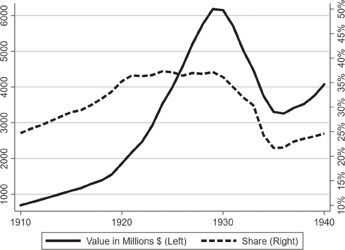
Figure 1 RISE AND FALL OF B&LS DURING THE INTERWAR PERIOD
Note: Notes: Value (in millions, on the left) and share of total institutional real estate lending (in percentage points, on the right) by building and loan associations in the United States.
Source: Carter et al. (2006).
This first B&L in the United States, the Oxford Provident Association in Frankfort, PA, followed what was known as the terminating plan. In a terminating plan, a group of households would get together to put forward funds for initial stock purchases in the association and commit to future savings. These funds were then auctioned to members, and the member who bid the highest for funds would obtain a mortgage loan from the association. The amount bid, the “premium,” was discounted from the gross amount the household was able to borrow. This mortgage was accompanied by periodic repayments toward interest, amortization, and installment on stock payments. As members saved and borrowers repaid, new members would then become borrowers. However, payments pre-specified the end date of the last mortgage’s payment, following which the institution was liquidated.
As the plan was inherently temporary, which ran counter to goals of long-term savings, B&Ls soon took on two related forms called the serial plan and the permanent plan. These plans allowed for several series of “withdrawable shares” to be issued, each maturing at different times. The serial plan, which came first, allowed different series of withdrawable shares to be issued at regular intervals so that new members no longer had to back-pay larger amounts of funds the later they entered the association. Instead, members would be on equal footing with others from the same series. The innovation of the permanent plan was that it allowed investors to purchase withdrawable shares without paying prohibitively large back payments to catch up to earlier members. In other words, members implicitly began their own new series when they joined. However, members still had to commit to a long-term savings plan, and these associations frequently had high withdrawal penalties.
Taking this idea to the limit, B&Ls eventually developed into a form known colloquially as the Dayton plan. Institutions using this plan allowed individuals to make payments whenever they pleased, rather than at a regular interval. There were typically lower withdrawal penalties, and members could usually withdraw money on request (Pieplow Reference Pieplow and David2013 [1931]). Dayton plans were most common in Ohio and a few other states in the country, including California. Dayton B&Ls frequently issued some sort of debt contract rather than relying solely on withdrawable shares. The Dayton B&Ls in Ohio actually accepted deposits, which led to the observation that the Dayton B&Ls were “open to the charge of being savings banks, a term frequently applied as a stigma” (Clark and Chase Reference Clark and Chase1927, p. 46). On the lending side, the premium on loans was eliminated for Dayton plans.
There were therefore two broad classes of B&Ls operating during the 1920s: Dayton plans, which were more closely related to commercial banks and catered to short-term investors, and non-Dayton plans (serial and permanent plans), which required more of a commitment by members. Both plans specialized in local real estate by permitting only their members to borrow. Table 1, taken from Clark and Chase (Reference Clark and Chase1927), shows the distribution in 1923 for the United States as a whole. Terminating plans were almost eliminated, accounting for less than 1 percent of the total. Serial or permanent plans accounted for 87 percent, while Dayton plans accounted for a little over 11 percent.
TABLE 1 DISTRIBUTION OF PLANS IN THE UNITED STATES IN 1923

Notes: “Serial/Permanent” calculated as the sum of “Serial” and “Regular Permanent” as defined by Clark and Chase (Reference Clark and Chase1927). Percent shares may not add up to 100 percent due to rounding.
Sources: Clark and Chase (Reference Clark and Chase1927, p. 61) and author’s calculations.
By 1935, the federal government had implemented a number of new laws targeting the B&L industry that made it possible for B&Ls to “federalize,” or join the Federal Home Loan Bank system (in a similar manner as commercial banks could become Federal Reserve banks). Snowden (Reference Snowden, Stanley, Philip, Rosenthal and Kenneth2003) discusses how these laws helped create the savings and loan industry that would persist for the following decades.
California Building and Loans
The reported history of B&Ls in California traces back to 1893, when the first annual report of the Office of the Board of Commissioners of the Building and Loan Associations was issued and the Building and Loan Commission was created. The earliest reports only mention plan type in passing and focus instead on whether members planned to become borrowers.Footnote 5 By the third annual report in 1895, the Dayton plan had begun to be used by two institutions in California. In the seventh annual report in 1900, California was well aware of the transition from Permanent/Serial to Dayton: “…the old Terminating association was succeeded by the Serial and is now fast being succeeded by the Dayton.” By 1905, this number had jumped to 24 officially listed. As described in detail by Haveman and Rao (Reference Haveman and Rao1997), although the Dayton plan grew in popularity, the coexistence of these different types of B&Ls continued throughout this time period and into the 1920s.
Non-Dayton B&Ls issued various forms of withdrawable shares, which, as previously described, were equity contracts featured elsewhere in the country (e.g., in New Jersey, as discussed by Fleitas, Fishback, and Snowden Reference Fleitas, Fishback and Snowden2018). There were two main forms of withdrawable shares: installment shares and full-paid shares. Installment shares created the forced savings plan, as individuals would commit to regular savings until their total savings reached the value of an individual withdrawable share. Full-paid shares allowed individuals to simply purchase the full value of an individual withdrawable share. Withdrawable shares typically had variable returns based on the dividends of the institution and featured costs of withdrawal.
Dayton B&Ls in California were unique in that they issued investment certificates, which distinguished them from other Dayton plans elsewhere in the country. Along with having lower withdrawal penalties relative to withdrawable shares, investment certificates were a type of debt contract that featured a fixed rate of interest. These investment certificates were senior to withdrawable shares in the event of liquidation (Stanford Law Review 1950; Bodfish Reference Bodfish1931). Clark and Chase (Reference Clark and Chase1927, p. 185) view these certificates as comparable with certificates of deposit, as they make it “possible to withdraw money quickly and take it elsewhere.” This made it easier to attract new members. Unlike withdrawable shares, California B&Ls were required to keep a reserve on hand for investment certificates of 10 percent for any amount up to $1 million, with an additional percentage that scales with the amount issued (e.g., 3 percent for any amount in excess of $5 million). This reserve could be composed of a standard reserve fund and/or what was known as “guarantee stock.”
Guarantee stock was another development in the evolution of both Dayton and non-Dayton plans. Guaranteed-stock plans allowed some members to purchase non-withdrawable stock in the institution, which was essentially the initial capital. This allowed the institution to begin making a higher volume of loans more quickly and guarantee some form of interest or dividend payouts for investment certificates and withdrawable shares, respectively. The institution could use this guarantee stock as a reserve for investment certificates and could also presumably respond more easily to withdrawal requests for both investment certificates and withdrawable shares by having some capital on hand. In California, most B&Ls had guaranteed stock by the end of the 1920s. While dividends were not guaranteed, guarantee-stockholders would typically receive excess earnings beyond those allotted to other liabilities.Footnote 6
The general shift toward Dayton plans reflects a financial environment motivated toward an efficient movement of funds in the face of large migrations into California.Footnote 7 Haveman and Rao (Reference Haveman and Rao1997) and Haveman, Rao, and Paruchuri (Reference Haveman, Rao and Paruchuri2007) argue that the shift toward the Dayton plan was due to values related to the Progressive movement. A desire for efficiency pushed B&Ls from club-like non-Dayton plans to bureaucratic Dayton plans. This change was propagated by internal migration and immigration into California, which expanded the size of local financial networks and reduced the ability to build long-term relationships. Dayton plans, attractive due to their low withdrawal fees and ease of access, began to grow. This general shift toward efficiency is similar to the overall transformation of California banking. As described by Doti and Schweikart (Reference Doti and Schweikart1991), a substantial portion of early banking along the frontier was highly localized. By the early 1900s, following a series of panics and dishonest bankers, state regulation began taking form and bank examiners began conducting regular examinations, thereby streamlining bank reporting. Doti and Schweikart (Reference Doti and Schweikart1991) argue that these examinations created opaque reports from the perspective of the depositor. Depositors increasingly relied upon the specialists’ determination of banking safety (even if such specialists were potentially unqualified and received the job due to political connections).
Taken together, both the Progressive movement described in Haveman and Rao (Reference Haveman and Rao1997) and the increasing reliance on specialists as in Doti and Schweikart (Reference Doti and Schweikart1991) suggest an important role for flightiness. First, shifting toward more efficient banking systems may have attracted newer members and depositors. These newcomers may not have been financially savvy and may instead have relied more on external regulators for safety. Second, as individual members grew wary of their fellow members or understood less about their local institutions, they may have been more likely to wish to withdraw funds in the event of a bad shock.
To withdraw funds in California, members would formally request to do so in writing with at least 30 days notice. The member would receive some amount up to the full value of what he paid in, although withdrawal values (especially for withdrawable shares) were frequently less than the book value. B&Ls were then required to use up to 50 percent of their receipts in a given month to respond to withdrawal requests. In California, associations were required to pay all withdrawal requests on file within a year, or all receipts would go toward withdrawals. This was also true for investment certificates, which were similar to deposits in that they represented debt. If withdrawals were not paid out within two years, the state commissioner would have the power to liquidate the B&L according to the 1929 Civil Code.
In California, the different plan types were evident in their advertisements. Non-Dayton plans would state the overall return and, in some cases, directly emphasize the forced savings component. The left panel of Figure 2 shows for the Guarantee Building and Loan Association in San Bernardino, a non-Dayton plan that closed in 1930, both the savings plan component (“save $10 every month for but six and a half year”) as well as the overall return (“[e]very dollar has earned 8 per cent return”). Compare this to the Dayton plan advertisements. The right panel of Figure 2 shows an advertisement for the Guaranty Building and Loan Association in San Jose, a Dayton plan in my sample that did not close. One of the key features of their investment plan is the advertised ability to withdraw essentially on demand. Advertisements such as these were documented in a B&L post-mortem, with the Select Committee of the California Assembly for the Purpose of Investigating the Building and Loan Situation in the State of California noting that “…a definite relationship between advertising and present conditions exists … those associations most active in advertising for new investors are those associations which are today suffering…” (Dawson et al. Reference Dawson, McBride, Utt and Louis Welsh1935, p.137). Even Commissioner Louis C. Drapeau noted in 1935 that “[t]he impressions that building and loan associations offered high interest on savings invested with them, and that investors could have their money returned to them at their demand, were eagerly accepted and believed by the average investor” (Drapeau Reference Drapeau1935, p. 127).

Figure 2 BUILDING AND LOAN ADVERTISEMENTS
Notes: The left panel shows an advertisement for a non-Dayton plan. The right panel shows an advertisement for a Dayton plan.
Sources: Non-Dayton Plan Advertisement: San Bernardino Sun, Volume 57, Number 31, Page 8 (1 October 1925); Dayton Plan Advertisement: Healdsburg Tribune, Number 54, Page 4 (9 January 1928); Accessed via UCR California Digital Newspaper Collection. Courtesy of the California Digital Newspaper Collection, Center for Bibliographic Studies and Research, University of California, Riverside, http://cdnc.ucr.edu.
Figure 3 shows the development of total assets and the total number of associations for reporting B&Ls from 1920–1934. As elsewhere in the country, during the 1920s, the number of associations and the total number of assets were on the rise. The number of associations peaked in 1929 at 233 associations, whereas the total value of assets peaked in 1930 at $513,110,594.58. Like elsewhere, there was strict regulation limiting California B&Ls to mortgage loans.Footnote 8 Figure 4 maps the location of B&Ls in California. As shown in the left panel, the location of B&Ls unsurprisingly tracks the population of the state.Footnote 9 The right panel of Figure 4 shows the distribution by plan type. Dayton plans were more common in the state but were not obviously overrepresented in any specific location.

Figure 3 CALIFORNIA B&LS IN THE GREAT DEPRESSION
Notes: Total assets (in millions, on the left) and total number (on the right) of California B&Ls over the period 1920–1935.
Source: Building and Loan Commissioner (various years).

Figure 4 COUNTY DISTRIBUTION OF CALIFORNIA BUILDING AND LOAN ASSOCIATIONS IN 1927
Notes: The left panel maps the total number of California B&L’s active in 1927. The right panel maps the share of Dayton plans. Both maps are at the county level.
Source: Building and Loan Commissioner (1927).
The explosive growth in B&Ls in California began to attract notice, and California state officials also started considering additional regulations.Footnote 10 Although B&Ls continued to increase in size through 1930, new commissioner Charles Whitmore wrote to the governor in the 1930 annual report that “Loan commitments by associations showed a decline for the year of 38 per cent” (Building and Loan Commissioner 1931, p. 13). However, he did not see any cause for concern, writing that “conditions in many parts of the state show signs of returning normality, and more and better loans are now being offered for association investment.”
The 1930s would be hard for B&Ls, as the total number operating in California declined from 233 total associations in 1929 to 178 associations in 1934.Footnote 11 In the 1932 annual report, new commissioner Friend W. Richardson, wrote that “[t]he year 1932 was the most critical in the history of building and loan associations” (Building and Loan Commissioner 1933, p. 3). Through 1934, the number of associations and the total amount of assets were on a steady decline, as was common throughout the country. The relatively high closure rates of the Dayton plans, which relied more on these investment certificates, were noted by contemporaries. In the Minority Report by the California Legislature, Chairman Frederick Peterson notes that “complaints were directed against stock organizations - particularly those … affiliated with companies dealing in pass book and investment securities.” His recommendation was the elimination of this system, emphasizing that B&Ls had led investors to see passbooks and investment certificates as deposits (Peterson Reference Peterson1935, p. 145).
Do B&Ls Fail?
B&Ls were fundamentally different institutions from commercial banks. Commercial banks’ main source of liabilities were depositors that owned debt contracts in the commercial bank. In the event that a bank could not pay out depositors, then the bank could be forced to close. However, for B&Ls, the withdrawable shares they issued were in fact equity contracts. This meant that along with the involuntary liquidation mentioned earlier, shareholders could choose to voluntarily liquidate B&L or merge with another association.
The voluntary liquidation option has been studied in the New Jersey context by Fleitas, Fishback, and Snowden (Reference Fleitas, Fishback and Snowden2018). In New Jersey, voluntary liquidation occurred when two-thirds of members, either borrowing or non-borrowing, voted to liquidate. Fleitas, Fishback, and Snowden (Reference Fleitas, Fishback and Snowden2018) find that the probability of liquidation rose when there was a higher share of non-borrowers. Similar laws were in place in California. Paragraphs 83 and 87 of the 1891 California B&L act dictated that “dissolution” could also be either involuntary (if the association commits a crime or an “unsafe practice”) or voluntary. In 1911, the commissioner was given the power to “revoke the license of any … association … [whose] solvency whereof may have become imperiled…” In California, voluntary dissolution always required a two-thirds majority, as in New Jersey.
Alternatively, members could theoretically sell their withdrawable shares (or investment certificates) in informal secondary markets. Rose (Reference Rose, Eugene, Snowden and Fishback2014) studies the markets in New Jersey but finds that these secondary markets are common throughout the country. There is evidence that these markets existed in California, as Rose (Reference Rose, Eugene, Snowden and Fishback2014) finds that as late as 1934, share prices in San Francisco were 50 cents on the dollar. However, Rose (Reference Rose, Eugene, Snowden and Fishback2014) finds that these markets were not fully mature until the late 1930s, making it unlikely that members could easily sell shares during the early stages of the Great Depression.
The closure of a B&L was a complex affair. Whether an association voted to close or chose to engage in a lengthy court battle to prove insolvency meant that, in some cases, years could go by before a result was determined. The analysis in this paper relies on the fact that closures were not necessarily quick but were driven by the shock of the Great Depression and occurred by 1935.
DATA
I draw on historical data on B&Ls in California. I focus on California for a number of reasons. First, California has a non-trivial share of non-Dayton and Dayton plans, unlike almost every other state in the country. Second, the amount of money invested, in terms of assets per member, was higher relative to the United States as a whole. In 1923, assets per member in California were $1,014.22 compared with $486.96 for the United States (Clark and Chase Reference Clark and Chase1927). Members in California presumably relied more heavily on B&Ls as a source of investment, making the B&L choice salient. Third, data availability makes California B&Ls attractive to study. Annual balance sheet and profit and loss data are available from the annual reports of the state’s building and loan commissioner. Additionally, select underlying archival data from the annual reports have survived to provide additional insight into how B&Ls operated during the Great Depression. Finally, California’s Building and Loan League was active in preventing so-called “National” B&Ls, or B&Ls headquartered outside of the state of California, from entering. Thus, nearly every B&L operated almost exclusively in California, limiting the effect of external factors in determining closure rates.
Public Annual Reports Data
I use the appendices to the 1927, 1929, 1930, and 1935 annual reports from the Building and Loan Commissioner in California to construct a cross-section of B&L balance sheets in California. The focus on these years is due both to data availability and economic history. The 1927 annual reports explicitly stated whether the institution was a Dayton plan. Data availability in 1927 was also at its highest. Along with balance sheets, which were available every year, the 1927 annual reports also have data on member contracts such as dues, withdrawal values, and dividends. The 1929 annual reports provide baseline balance sheet characteristics just prior to the onset of the Great Depression, avoiding any effects from depressed aggregate economic conditions.Footnote 12 This implicitly assumes that the onset of the Great Depression was sufficiently unexpected that the decision to start and operate a B&L by 1929 was independent of this aggregate shock. I use the cash-flow statements from the 1927 and 1930 annual reports, as the 1929 annual report does not include this information. I obtain the operating status from the 1935 annual report, which includes the effects of the Great Depression and limits the effects of federal programs, such as the Federal Home Loan Bank System, that may affect decisions to remain open.
An example of a balance sheet in 1927 for a Dayton B&L is displayed in the left panel of Figure 5. Above the balance sheet is demographic information about the B&L, such as the number of members/investors and shares (which appear to include both withdrawable shares and investment certificates). In the middle of the page is the balance sheet data. On the asset side, the large reliance on real estate loans is clearly visible. On the liability side, we can see the importance of investment certificates (listed as the third item). Finally, at the bottom of the page, one can see clearly that the association is labeled “Dayton Plan.” There is also additional data on dues and withdrawal values. The right panel of Figure 5 presents a non-Dayton plan. The key differences are the reliance on withdrawable shares as liabilities rather than investment certificates and the listing of individual series at the bottom of the page. From the 1929 annual report, I record the complete balance sheet of each B&L. From the 1927 annual reports, I record the total number of members, the total number of shares, dues per certificate or withdrawable share, and any description of withdrawal value. While dues per share could differ across series for non-Dayton plans, in practice they did not.

Figure 5 BUILDING AND LOAN ASSOCIATION BALANCE SHEETS
Notes: Left panel shows a sample B&L balance sheet for a Dayton plan (as indicated at the bottom of the figure). Right panel shows a sample B&L balance sheet for a non-Dayton plan.
Source: Building and Loan Commissioner (1927), courtesy of HathiTrust.
Using the reported plan type from the 1927 annual report should well represent the operations of the B&L, particularly how the managers aimed to attract new members. However, this measure ignores the fact that many B&Ls issued both withdrawable shares (typical of non-Dayton plans) and investment certificates (typical of Dayton plans). I construct an alternative measure by considering only the observed liability structure of the balance sheet. B&Ls reported “withdrawable shares” separately from “investment certificates.” I calculate the share of investment certificates relative to the sum of investment certificates and withdrawable shares in 1929 for a given B&L. I discretize this measure by comparing it to the median value across B&Ls. I call this the “liabilities” measure of the Dayton plan. Figure 6 shows, for Dayton and non-Dayton plans, the ratio of investment securities to the sum of investment securities and shares, meant to capture how much of a B&L’s standard liabilities are in one or the other.Footnote 13 The preferred specification is to use the reported measure rather than the liabilities measure, as this probably more accurately captures the managerial decisions of how to attract new members, but I present results using both measures.

Figure 6 INVESTMENT CERTIFICATES SHARE OF LIABILITIES
Notes: The share of investment securities is calculated as the ratio of investment certificates to total liabilities in 1929.
Sources: Building and Loan Commissioner (1929, 1927).
From the 1935 annual report, I record the operating status of B&Ls and the year in which the institution ceased operating. The reasons for ceasing operations are listed as one of the following: absorbed, removed, consolidated, transferred, merged, revoked, federalized, and liquidated (both voluntary and involuntary). I classify as closures those listed as absorbed, liquidated, transferred, and consolidated.Footnote 14 If the business is listed as removed, I classify them as open, as these represent relocations or name changes. I drop B&Ls that closed prior to 1929. There are 55 closures from the 1927 listing of B&Ls in my sample. This number rises to 76 closures when using the liabilities measure, which relies on 1929 balance sheets (and so includes B&Ls started in 1927, 1928, and 1929).Footnote 15
The final sample contains 164 non-federalized B&Ls active in 1927 and 205 non-federalized active in 1929. In California in 1927, there were significantly more Dayton plans than non-Dayton plans. This is true not only in the state as a whole but also within counties. From Figure 4, which shows the distribution of B&Ls and their types, we can see that the majority of counties with at least one B&L also have at least one of each type.
Archival Data
I hand-record surviving archival data available from the CSA in Sacramento, California. I use raw copies of the detailed balance sheet data submitted by the B&Ls that were maintained by the Los Angeles office.Footnote 16 These recordings form the basis of the balance sheets in the annual reports. Along with the publicly available information, they also include additional statistics such as lending rates and member returns.
These unpublished recordings contain a wealth of useful information.Footnote 17 I observe the reported interest on mortgage lending, either the average or, in some cases, simply a list or range of interest rates on loans currently outstanding. There are also details on the average rate of interest on investment certificates. These archival reports are only available at five-year intervals for a limited number of B&Ls (specifically, 1926, 1931, and 1936). I focus on the 1931 annual reports, which is the earliest year for which a substantial number of B&Ls have surviving balance sheet data.Footnote 18 I hand-match these data to the 1927 and 1929 balance sheet data. I am only able to match around half of the sample. For the remainder, the B&Ls either closed before 1931 or the reports did not survive.
Summary Statistics
Summary statistics for the set of 205 non-federalized B&Ls with 1929 balance sheet information are reported in Table 2. This table includes merged city- or county-level data from a variety of other sources.Footnote 19 Of the 164 institutions with 1927 balance sheet information, approximately three-quarters report as Dayton plans. Of the 204 institutions with balance sheet data in 1927, around 37 percent of B&Ls closed according to my definition. The average number of members and assets is around 1,400 and $2 million, respectively, although the largest B&Ls had 9,000 members and $30 million in assets in 1929.
TABLE 2 SUMMARY STATISTICS

Notes: “Dayton (reported)” and “Members (thousands)” use data from the 1927 annual reports and so drop B&Ls formed in 1927–1929. “Closure dummy” is a dummy variable equal to one if a building and loan association was absorbed, liquidated, consolidated, or transferred by 1935. “Age (years since incorporation)” calculated as the number of years since incorporation as of 1929. “Investment securities share of member funds” calculated as investment securities divided by the sum of investment securities and withdrawable shares.
Sources: Building and Loan Commissioner (1927, 1929, 1935), Bleemer (2016), and Carlson and Mitchener (2009).
To better understand the differences across institutions, a balance table for non-Dayton and Dayton plans is presented in Table 3. Some key differences stand out. First and foremost, non-Dayton B&Ls were older. This is not unexpected; the historical development of B&Ls and the relatively recent development of the Dayton plan development predicts this age difference. Second, turning to balance sheet variables, Dayton plans were larger in terms of both assets and members. Third, unsurprisingly, the composition of balance sheets differs as Dayton plans relied overwhelmingly more on investment certificates in their liabilities (including guarantee stock), while non-Dayton plans relied more heavily on withdrawable shares. Both make up more than half of their liabilities on average. If anything, Dayton B&Ls had more liquidity available in terms of cash ratios. Part of this was due to the legal requirements for maintaining reserves when issuing investment certificates. Dayton plans were also more likely to be located in larger cities with more commercial banks.
TABLE 3 DAYTON AND NON-DAYTON (REPORTED) BALANCE TABLE

Notes: “Dayton (reported)” and “Members (thousands)” use data from the 1927 annual reports and so drop B&Ls formed in 1927–1929. “Closure dummy” is a dummy variable equal to one if a building and loan association was absorbed, liquidated, consolidated, or transferred by 1935. “Age (years since incorporation)” calculated as the number of years since incorporation as of 1929. “Investment securities share of member funds” calculated as investment securities divided by the sum of investment securities and withdrawable shares. Heteroskedasticity robust standard errors in parentheses. *p < 0.1, **p < 0.05, ***p < 0.01.
Sources: Building and Loan Commissioner (1927, 1929, 1935), Bleemer (2016), and Carlson and Mitchener (2009).
In Online Appendix B, I show which factors play a predictive role in determining B&L plan choice.Footnote 20 Age is by far the most important predictor of the Dayton plan. In all cases, the age variable is highly significant. Conditional on age, of the observable local variables only the log population is marginally significant. This result is consistent with the argument in Haveman and Rao (Reference Haveman and Rao1997) that Progressive values and the desire for more efficient institutions in response to immigration led to the adoption of the Dayton plan.
CLOSURE RATES
I first show that the probability of closure for Dayton B&Ls was higher relative to non-Dayton B&Ls. I estimate the following regression model via ordinary least squares (OLS)
 $$Closur{e_i} = \alpha + \beta Dayto{n_i} + \Gamma {X_i} + {\varepsilon _i},$$
where Closure i is a dummy variable equal to one if B&L i closes between 1929 and 1935, Dayton i is a dummy variable equal to one if the institution is a Dayton plan, X i is a vector of controls potentially at the B&L level, and ε i is the error term. The coefficient of interest, β, represents the relative increase in closure rates for Dayton plans compared with non-Dayton plans. This coefficient is hypothesized to be positive, indicating that Dayton B&Ls were more likely to close. I show results using both the reported and liability measures of Dayton status.
In a causal sense, the identifying assumption in this model is that the decision of whether or not to use the Dayton plan, or issue relatively more investment certificates, is uncorrelated with other determinants of closure that would be included in the error term ε i. Some threats to this assumption are observable and can be directly controlled. First, the size of B&Ls may be an indicator of distress. If larger B&Ls are more diversified or more efficient, then the coefficient β may be biased, as Dayton B&Ls were on average slightly larger. To account for this possibility, I include log assets as a control in X i. Second, the age of the institution is frequently found to be an important determinant of closure. I use age group dummies to account for this concern.Footnote 21 The third threat to identification is the vulnerability of the B&L due to the maturity mismatch of the balance sheet. While I have already argued that the structure of the asset side of the balance sheet is similar for both types of B&Ls, liquidity ratios differed across institutions. For example, all plans were required to hold reserves against the outstanding value of investment certificates. This would naturally imply that Dayton plans, which issued more investment certificates, had higher liquidity ratios. I include the cash ratio as a control to account for this possibility.
Another threat to identification is local economic conditions, such as the size of the local population or commercial bank competition. Local banking competition may push B&Ls to take the Dayton plan. This competition may also result in higher closure rates if banking panics spread locally. This would bias the estimate of β upwards. I include both the log population and the log number of commercial banks in the city as controls to account for this possibility. I also show that the results are robust to the inclusion of city-fixed effects.
The estimates of β support the hypothesis that Dayton plans did close at higher rates. Table 4 reports the results from estimating Equation (1) via OLS (Messer 2022).Footnote 22 The first column reports results from the bivariate regression of closure on only the reported Dayton measure (without any controls). The point estimate of 0.224 (SE: 0.07) implies that Dayton institutions had higher closure rates on the order of around 22 percentage points. The second column includes B&L size and balance sheet controls. The coefficient β changes only slightly to 0.238 (SE: 0.08) but remains significant both economically and statistically. In the third column, I include the age dummies and the coefficient estimate again remains broadly unchanged, but note that the standard errors widen due to the high correlation between age and plan type. Finally, the fourth column reports results including the local controls, and the point estimate falls slightly but remains significant and of similar magnitude. I repeat this ordering in the last four columns using the liabilities measure of the Dayton plan, and a similar pattern emerges.
TABLE 4 CLOSURE RATES REGRESSION RESULTS

Notes: Estimation results for the coefficient β from estimating the equation Closure i = α + βDayton i + ΛXi + εi. Closurei is a dummy variable equal to one if building and loan association i was absorbed, liquidated, consolidated, or transferred by 1935. Daytoni is an indicator variable equal to one if the institution is a Dayton plan. “Dayton (reported)” is the plan type as reported in the 1927 annual reports, while “Dayton (liabilities)” is a dummy variable equal to one if the association has above-median investment certificates as a share of liabilities. B&L controls include log assets and cash percentage. Age controls include age bin fixed effects. Local controls include log city population and log number of commercial banks in the city. Heteroskedasticity robust standard errors in parentheses. *p < 0.1, **p < 0.05, ***p < 0.01.
Sources: Building and Loan Commissioner (1927, 1929, 1935), Bleemer (2016), and Carlson and Mitchener (2009).
The results are robust to a number of different specifications and sample selection decisions. Table 5 re-estimates the benchmark specifications under alternative specifications. The first column simply replicates the third column of Table 4 for convenience. The second column includes city-fixed effects. The third column restricts the results to counties with at least one of each type of B&L present (while still including city-fixed effects), and the estimate is unchanged. Finally, the fourth column drops the two largest counties: San Francisco and Los Angeles (still including city-fixed effects). Although Los Angeles had a large number of closed Dayton plans, the fact that the results were robust after dropping these cities is strong evidence of the importance of plan type. The next four columns again focus on the liability measure. A similar pattern emerges, and the results are highly significant with city-fixed effects across all specifications.
TABLE 5 CLOSURE RATES: ALTERNATIVE SPECIFICATIONS

Notes: Estimation results for the coefficient β from estimating the equation Closurei = α + βDaytoni + ΛXi + εi. Closurei is a dummy variable equal to one if building and loan association i was absorbed, liquidated, consolidated, or transferred. Daytoni is an indicator variable equal to one if the institution is a Dayton plan. “Dayton (reported)” is the plan type as reported in the 1927 annual reports, while “Dayton (liabilities)” is a dummy variable equal to one if the association has above-median investment certificates as a share of liabilities. B&L controls include log assets and cash percentage. Age controls include age bin fixed effects. The sample denoted “Full” is the benchmark sample of 164 B&Ls for the reported measure and 205 B&Ls for the liabilities measure. The sample denoted “Both” includes only counties which contain at least one of each type of B&L (Dayton and non-Dayton). “No SF/LA” drops B&Ls located in San Francisco or Los Angeles. Heteroskedasticity robust standard errors in parentheses. *p < 0.1, **p < 0.05, ***p < 0.01.
Sources: Building and Loan Commissioner (1927, 1929, 1935).
The results in this section strongly support the hypothesis that Dayton plans had closure rates that were significantly higher than non-Dayton plans. In the next section, I dig deeper into the mechanism driving this result by using information on access costs, returns, and measures of liquidity needs. Before proceeding, I discuss several robustness checks regarding the stability of the results when including additional controls. I then briefly discuss additional checks available in the Online Appendix.
Robustness Checks
In the Online Appendix, I investigate the stability of the coefficient estimate subject to other controls in order to address various identification concerns.Footnote 23 I show that the results are not sensitive to balance sheet measures of borrower quality. If Dayton plans borrowers were more ex-ante likely to default in general, then the differential closure rates I identify may simply be due to the impairment of assets. Real estate-owned shares are a useful proxy for default risk. As emphasized by Fleitas, Fishback, and Snowden (Reference Fleitas, Fishback and Snowden2018), this asset includes foreclosed property taken on by the B&L. The results are robust to the inclusion of this control. I also show that the ownership structure of the B&L is not a concern. Fleitas, Fishback, and Snowden (Reference Fleitas, Fishback and Snowden2018) discuss how B&Ls in New Jersey could close with a 2/3 majority vote by shareholders and stockholders. The regulations on closure were similar in California. I construct a “concentration index,” which is the sum of withdrawable shares and guarantee stock as a share of assets. This measure captures how much the B&L relied on voting members. Including this measure does not affect the point estimate.
I also show that dropping either involuntary closures or consolidations and transfers does not significantly affect the results. Dropping involuntary closures homes in on the liquidity decision by focusing on whether members would be willing to liquidate the institution to access funds. Dropping consolidations and transfers is a robustness check on the classification of closure codes. I also examine the decision to federalize. B&Ls that may have liquidated might instead choose to federalize instead. Due to the distress faced by B&Ls during the Great Depression, U.S. federal policy in the 1930s allowed B&Ls to federalize and join the Federal Home Loan Bank system, created in 1932. In the Online Appendix, I show that treating federalization as either closure or as an independent outcome in a multinomial logit framework does not affect the results. I also show that the results are not sensitive to survivor bias on the part of non-Dayton plans that survived earlier recessions.
COSTS, RETURNS, AND LENDING RATES
In this section, I investigate why there were higher closure rates at Dayton plans by focusing on the characteristics of the B&L plans’ liability structures. I first show suggestive evidence that non-Dayton B&Ls had higher access costs and higher withdrawal penalties for members. To account for higher access costs, I then leverage the archival data to show that non-Dayton B&Ls attracted members by offering higher returns; however lending rates and loan characteristics were largely equal across the institutions. Taken together, I argue that this framework resulted in less flighty members (ex-ante less likely to need to access their funds during a shock). As additional evidence, I use reported withdrawal fees during the Great Depression to show that liquidity needs seemed higher at Dayton plans. For brevity, I focus on the reported measure of Dayton status in the tables that follow.Footnote 24
Access Costs: Withdrawal Fees and Dues
I begin by comparing the withdrawal penalties across plans in California. As elsewhere, withdrawal penalties could be in the form of timing restrictions or fees. The first page of the 1927 annual report notes that “many associations in the past have advertised that money might be withdrawn at will by the investor, and the public has come to expect it,” suggesting that in some cases individuals tended to believe they could withdraw on demand with little to no penalty. In California, withdrawals of both withdrawable shares and investment certificates were subject to up to 30 days’ advance notice. Withdrawal fees in California were more lax than in other parts of the country. Clark and Chase (Reference Clark and Chase1927) note that California is one of only two states that does not permit forfeiture of principal when investors withdraw either installment shares or investment certificates. Instead, entrance fees or withdrawal fees are charged. Clark and Chase (Reference Clark and Chase1927) note that these fees may be high enough to effectively reduce the principal if an investor withdraws too early.
Withdrawal penalties were not explicitly listed in the 1927 balance sheets. Instead, information regarding the value of withdrawals was presented. Clark and Chase (Reference Clark and Chase1927, p. 169) state that “[a]ssociations using the Dayton plan … customarily repay to withdrawing members the full book value of their investment.” This statement suggests that withdrawal fees are low and that whether a member receives book value is a good measure of withdrawal cost. The appendix to Clark and Chase (Reference Clark and Chase1927, p. 522) also describes withdrawal fees as “Deductions from book value when shares are withdrawn before maturity.”
For Dayton plans, withdrawal values were listed in the 1927 annual report as either “Full Book Value” or “Dues plus Profits.” I treat Dues plus Profits as a withdrawal penalty. Relative to book value, profits were more variable and were paid out only on specific dates.Footnote 25 The 1891 annual report in California also found that the average amount of profits paid out was only 50 percent of the total accrued, suggesting this is a good measure of withdrawal penalties. Non-Dayton plans explicitly listed the withdrawal value for each share series, as shown at the bottom of Figure 5. If this withdrawal value was less than the listed book value, then I consider this a withdrawal penalty under the definition by Clark and Chase (Reference Clark and Chase1927). In no case is the total withdrawal value less than dues, so the penalty is on the returns rather than the principal itself.
I compare withdrawal costs using the benchmark regression specification as in Table 4, but set the outcome variable to be a dummy equal to 1 if an institution has withdrawal penalties.Footnote 26 The first column of the top panel of Table 6 shows that Dayton plans were significantly less likely to have withdrawal penalties (after controlling for B&L and local controls), being lower by around 50 percent, using the reported measure and conditional on observable B&L characteristics.
TABLE 6 EVIDENCE ON THE ROLE OF FLIGHTINESS IN PREDICTING CLOSURE

Notes: The top and middle panels show results from estimating the equation yi = α + βDaytoni + ΛXi + εi. Daytoni is an indicator variable equal to one if the institution is a Dayton plan. “Dayton (reported)” is the plan type as indicated by the 1927 balance sheet. The outcomes for the top panel include: “Withdrawal penalty,” a dummy equal to one if a B&L has penalties for withdrawing funds; “Dues,” the cost of dues in 1927; “Shares per member,” the ratio of total shares to total members; “Costs,” the product of “Dues” and “Shares per member” or total costs per member. The outcomes for the middle panel include “Return,” the weighted average of returns for investment certificates and withdrawable shares, where the weights are given by the relative proportion of each; “Borrower share,” the share of members that are borrowing, “Lending rate,” the average rate on mortgage loans, and “Log avg loan size,” the log of the ratio of the amount of loans to the number of loans. B&L controls include log assets and cash percentage, and age controls include age bin fixed effects. Age controls for the middle panel, which uses archival data, include a dummy equal to one if the association was incorporated after 1920 due to the limited sample size. The bottom panel estimates differences-in-differences specifications of the form yit = αi + βt + γ(Daytoni × 1(t = 1930)) + εi where αi and βt are association and time fixed effects respectively and 1(t = 1930) is a dummy equal to one if the year is 1930. The outcome yi is the ratio of fees to total assets. Heteroskedasticity robust standard errors in parentheses. *p < 0.1, **p < 0.05, ***p < 0.01.
Sources: Building and Loan Commissioner of the State of California (1927) and Department of Savings and Loan Records.
I next analyze costs as proxied by dues. Dues are what is owed at each meeting for forced savings plans. The traditional Dayton plan, as in Ohio, would not have any dues listed, but in California, there could be forced savings plans even for investment certificates. For my purposes, I am interested in whether these dues were different between Dayton and non-Dayton B&Ls. If the dues structure is lower at Dayton plans relative to non-Dayton plans, then this means that the forced savings plan for Dayton plans was less restrictive, which I consider to be a lower cost. Dayton plans listed the dues per share (or per certificate) per month, and this appeared to be the same amount for all members. Non-Dayton plans listed dues per share for each series, as shown in Figure 5.Footnote 27 I compare dues directly in the second column. Dues per share were around 10 cents lower for Dayton plans according to the reported measure, or just over half of a standard deviation.
Comparing only dues per share leaves out the fact that members of non-Dayton B&Ls may hold fewer shares in total. This would mean that the total amount of dues paid could be the same across institutions. To account for this possibility, I examine the number of withdrawable shares and certificates per member. The third column shows that Dayton B&Ls had significantly lower log shares per member. In the last column, I show that a measure of total cost of dues per member (or the product of columns two and three) is approximately $6 less for Dayton institutions compared with non-Dayton institutions. Since Dayton plan total costs were only around $4.75 per member, then non-Dayton plans essentially had significantly higher costs.
In sum, the detailed data on withdrawal penalties and costs, when paired with the historical narrative, provide indicative evidence that accessing funds was more difficult at Dayton plans. In addition, members at Dayton plans had higher costs of membership, not only because they held more shares on average but in part because Dayton plans charge lower dues.
Archival Data: Investor Return and Borrower Characteristics
Having presented evidence that access costs were higher at non-Dayton B&Ls, I now use the archival data to study returns and lending rates. The detailed annual statements in the archives provide information not available in the publicly available reports.Footnote 28
I begin by showing that returns were higher for non-Dayton plans. I calculate returns as the weighted average of listed returns on withdrawable shares and investment certificates, where the weights are given by the relative share in 1929 liabilities. The first column of the middle panel of Table 6 shows regression results of the observed investor rates on a dummy variable equal to 1 if an institution is listed as a Dayton plan, again controlling for B&L and local controls.Footnote 29 Dayton plans were associated with returns that were lower by around 23 basis points. Relative to variation in lending rates, this difference is economically meaningful. Returns, on average, were around 6 percent with a standard deviation of 37 basis points, so the result is approximately one-third to two-thirds of a standard deviation.Footnote 30
High returns alone do not imply that investors are being compensated exclusively for giving up liquidity access. First, high returns could compensate members for their time screening or monitoring loans issued. This is unlikely to be the case. Even if the withdrawal fee is a screening tool for potential borrowers, it only matters for the share of members that plan to borrow. For the remaining members, this fee purely affects liquidity access. While the early history of B&Ls in the 1800s involved members who were specifically looking to finance a home, by the 1920s and 1930s, advertisers were clearly stressing joining B&Ls purely for savings reasons. In fact, as shown in the next column, the ratio of borrowers to members was, if anything, lower at Dayton plans.
Second, one may be concerned that returns reflect a risk premium and compensate members for extending lower-quality loans. The third column of the middle panel of Table 6 shows that lending rates were similar or even higher at Dayton plans by around 30 basis points. However, it is likely that the net lending rates were more equal than this simple comparison suggests. Dayton plans had eliminated the premium (the amount, bid by the borrower, by which the gross value of the loan was reduced). Dayton plan members and borrowers likely internalized the premium, reflecting it in the lending rate rather than the net amount borrowed. Finally, average loan sizes are roughly similar across the institutions, as shown in the last column. Loans do not appear to have been riskier simply because they were bigger.
It is important to reiterate that all lending rates and returns are as of 1931 due to data availability. The regulatory landscape during the Great Depression significantly changed due to the passage of the Building and Loan Act in 1931, which made data collection a priority. Using 1931 excludes B&Ls that closed in the late 1920s, many of which were Dayton plans. One concern is that the Dayton plans that closed had offered high interest rates on investment certificates that they were unable to pay out, and thus closed. Unfortunately, given the data restrictions, I cannot exclude this as a possible explanation.
Member Liquidity Needs
I now argue that the potential liquidity needs were higher for members of Dayton plans than non-Dayton plans. I have already shown evidence that members at Dayton plans held fewer withdrawable shares or investment certificates than those at non-Dayton plans. If par values were similar and individuals invested the same share of wealth at B&Ls across types, then this would suggest that members of Dayton plans were of lower wealth than members of non-Dayton plans. Unfortunately, it is not immediately clear what the par value per share is from the available data, and without information on member characteristics, it is even less clear whether investment behavior differs across plan type.
A straightforward way to observe liquidity needs is to ask whether members were willing to pay costly fines, fees, or penalties to either access funds or stop regular savings plans during the Great Depression. Why would fees be a good way to measure liquidity needs? Clark and Chase (Reference Clark and Chase1927, p. 161) describe such fees as being an important tool to ensure regular savings. They note that “[i]t is well known that fees, fines, and forfeitures were originally designed to encourage persistence in saving.” If such fees are in place to encourage thrift, then it follows that whenever members are willing to pay, it is to deviate from savings plans due to liquidity needs.
I calculate the relative increase in fees paid during the Great Depression. In 1927 and 1930, the profit and loss accounts on the annual statements included various measures of fees. As the categories listed are different in the two years I record, I define as fees any line item that uses the words “fines” or “fees.” I then calculate the sum of all fees and divide it by the total assets in 1927. By dividing by assets in 1927, all changes are due to changes in fees, and total assets scale the outcome variable. One issue with this definition is that it includes fees paid by borrowers who are late on repayment, thereby including some measure of ex-post asset quality. However, as I have attempted to argue in this paper that asset quality is relatively similar across institutions, the difference in fees paid across institutions should largely reflect liquidity needs. Additionally, I can econometrically account for this difference.
I estimate the following regression:
 $$Fees\_Asset{s_{it}} = {\alpha _i} + {\gamma _t} + \lambda (DAYTO{N_i} \times 1(t = 1930)) + {\varepsilon _{it}},$$
where Fees_Assets it denotes fees relative to total assets (in 1927), DAYTON i is a dummy equal to one if the institution is a Dayton plan, and 1(t = 1930) is a dummy equal to 1 if the year is 1930; α i and γ t are B&L and time-fixed effects, respectively.
The main coefficient of interest is λ, which represents the relative increase in fees during the Great Depression for Dayton plans, relative to non-Dayton plans, compared with tranquil times (prior to the Great Depression). I hypothesize that λ > 0, which means that fees rose relatively more for Dayton plans relative to non-Dayton plans. This would imply that members at Dayton plans were more willing to pay to withdraw their money, or at least stop using their savings plans, than those at non-Dayton plans. I treat this as a test of liquidity because it implies that funds are more needed outside of a savings vehicle than inside.
This specification is a standard 2x2 differences-in-differences. The identifying assumptions are parallel trends (the difference in the outcome would have been the same in the absence of treatment) and exogeneity of treatment. I have already argued in this paper that the decision to have a Dayton plan is orthogonal to the beginning of the Great Depression, and so plans should not have been chosen anticipating this event. As for parallel trends, it is not possible to provide pre-trends as there are no data in the pre-period. Even so, the parallel trend assumption is likely to hold. The specification allows for differential levels of fees across plan types. What would be problematic is if Dayton plans were to increase or decrease fees over time relative to non-Dayton plans. However, there is no evidence that Dayton B&Ls were disproportionately raising or lowering fees. If anything, Dayton plans would be lowering such fees to continue to compete with local banks, meaning any estimate of λ would likely be a lower bound.
This specification is an imperfect test of liquidity needs for two reasons. First, this is a test of ex-post liquidity needs, not ex-ante. The main hypothesis of this paper is that Dayton B&Ls attracted individuals with higher liquidity needs, thereby endogenizing the probability of closure. Second, it could be the case that members at Dayton plans simply lost their jobs or sources of income. While this could be seen as a liquidity shock, it could also be interpreted as a net worth shock on the part of members. Taken together, this test is only suggestive of liquidity needs, assuming individuals understand the risks ex-ante. However, it is arguably the best test I could perform.
The last panel of Table 6 presents the results. The first column shows results using the reported measure for the 149 B&Ls with cash flow data in both 1927 and 1930. The point estimate of 0.792 (SE: 0.24) on the interaction term suggests that there was a rise in fees as a share of total assets by approximately 0.79 percentage points. This provides evidence that liquidity needs were an important difference between Dayton and non-Dayton B&Ls.
DISCUSSION
The Flightiness Mechanism
In practice, how might flightiness have contributed to B&L closure? First, Dayton plan members could have been more aggressive in requesting a withdrawal. Given the rule in California that required institutions to pay out withdrawals within two years, such aggressive demands would result in liquidation, potentially by the commissioner, if they occurred relatively quickly. Second, Dayton plans, which typically featured guarantee stock and non-voting investment certificates, may have elected to liquidate quicker as the equity value of the institution fell. The equity value may fall if either existing members’ demand for liquidity raised the chances of insolvency or if the B&L became unattractive to potential future members.
Both methods are likely to have occurred. Investment certificates (along with assets, as shown in Figure 3) peaked in 1930. However, closure rates only began to spike in 1930, suggesting two distinct waves. Table 7 shows how closures evolved over the Great Depression in California across types of closure. The first wave, in 1929–1930, experienced high numbers of consolidations and transfers. The second wave, while investment certificates were declining after 1930, experienced a higher rate of involuntary closures. Both periods are indicative of flighty members, albeit for different reasons.
TABLE 7 CLOSURE TYPE OVER TIME

Notes: Total closures by year and type. “Involuntary” includes any involuntary closure that results in liquidation or reorganization by the commissioner. “Other” includes absorption or voluntary liquidation.
Source: Building and Loan Commissioner of the State of California (1935).
The first period, through 1930, saw a rush into investment certificates by members seeking safety and liquidity, with the assumption that their investments would be easily withdrawable. Dayton plans, which marketed their investment certificates as precisely that, were happy to take the new members. The wave of consolidations and transfers may then represent a desire to reorganize B&Ls to take advantage of the high demand. Specifically, the consolidations and mergers resulted in chains of buildings and loans operated by one holding company. This transformation largely eliminated the “local contacts and local sympathies, which were originally important characteristics of building and loan associations” (Building and Loan Commissioner 1931, p. 8). Flighty members, whose focus was easy access to funds in the event of economic distress, were a symptom.
The period after 1930 featured involuntary withdrawals. The sharp increase in investment certificates in the first wave was the precondition for the next wave after 1930. In this period, flightiness directly determines closure for any of the three potential reasons mentioned earlier in this subsection. Indeed, splitting the sample into closures in 1929–1930 and closures after 1930 shows a strong effect in this latter period for Dayton plans.Footnote 31
Relation to Bank Failure Theory
This paper provides empirical results that help inform the theoretical literature on bank failure. I find that bank liquidity shocks can be endogenous to the depositor base, which in turn is a function of the types of liabilities issued by the bank. Multiple equilibrium models that feature liquidity shocks, such as the benchmark model of Diamond and Dybvig (Reference Diamond and Dybvig1983), typically assume that the probability of a liquidity shock is exogenous or at least that heterogeneity across depositors is orthogonal to the decision to withdraw funds. My results instead suggest an important role for depositor heterogeneity. One method of obtaining endogenous liquidity probabilities is to augment a bank failure model by allowing individuals to receive signals (e.g., Goldstein and Pauzner Reference Goldstein and Pauzner2005). These models typically emphasize signals about the health of the bank or the economy. In contrast, my results suggest that signals may also be a function of the characteristics of depositors. Alternatively, there are models of banking panics with a risk-averse set of agents (Caballero and Simsek Reference Caballero and Simsek2013) or models studying flight to safety (Caballero and Farhi Reference Caballero and Farhi2018). My results stress that heterogeneity across instruments determine whether an institution’s liabilities are held by such risk-averse agents.
The choice of how to structure liabilities to take into account asymmetric information about the flightiness of investors also has empirical support in my study. Offering investment contracts that any investor could purchase could be problematic in the event of a bad shock if such contracts attract flighty investors. B&Ls in California essentially engaged in a form of price discrimination across institutions. High-return, high-cost B&Ls attracted investors less likely to force a closure, while low-return, low-cost B&Ls were more likely to close. Whether these closures are efficient is beyond the scope of this paper.
Whether penalties are efficient is related to a separate but related class of models that studies how liquidity mismatch can be a commitment device (e.g., Calomiris and Kahn Reference Calomiris and Kahn1991). That depositors can easily withdraw funds may act as a check on the management practices of banks, especially if depositors respond to negative news by switching banks. It is not clear whether withdrawal penalties would reinforce or limit this channel. Because it is more difficult to withdraw, bank managers may be less likely to perform due diligence on new lending. However, if flightiness is negatively correlated with financial sophistication, management may feel pressure to make higher-quality investments lest a larger base of informed/sophisticated depositors leave.
CONCLUSION
In this paper, I study the role that flightiness plays in causing financial distress. I leverage institutional differences across B&Ls in California during the Great Depression. These institutions offer a unique laboratory to investigate flightiness because their liabilities greatly differ, with one type of plan, Dayton plans, offering relatively low withdrawal penalties and allowing irregular savings plans. At the same time, the asset structure across institutions was very similar and focused almost exclusively on mortgage lending.
I emphasize three main results. First, Dayton plans had a higher probability of closure during the Great Depression than other plans. Second, Dayton plans were less costly for members to join and participate in compared with other plans. Finally, Dayton plans had lower returns to members compared with non-Dayton plans. Taken together, these three results suggest that the access costs of non-Dayton B&Ls were an important factor in reducing closure rates, likely because they attracted a less flighty member who would be significantly less likely to need liquidity during the Great Depression. These higher withdrawal penalties were justified by offering higher returns to members.
The results in this paper do not necessarily imply that withdrawal penalties are socially optimal. As shown in this paper, B&Ls with withdrawal penalties also needed to pay out higher returns to members to attract investment in general. The need to pay out higher returns may affect lending rates and reduce demand for loanable funds, with potential spillover effects on local households and businesses. Future research can examine this tradeoff.
The evolution of Dayton B&Ls has important implications for financial stability. First, some of the liquidity characteristics of liabilities can lead to financial instability. During the Great Recession, both money market mutual funds and investment banks such as Lehman Brothers experienced distress (Gertler and Gilchrist Reference Gertler and Gilchrist2018). This distress took the form of a bank run in wholesale lending markets, where investors could easily withdraw funds. Capital flows are known to be fickle in international finance (e.g., Caballero and Simsek 2020). Central bank digital currencies (CBDCs), which represent a more liquid and low-cost alternative to bank deposits, may be an arguably safer asset available to the private sector. If households have access to CBDCs (so-called retail CBDCs as described by Boar and Wehrli Reference Boar and Wehrli2021), this arguably safer asset may lead to financial instability in future downturns if the retail holders of standard bank deposits are “flighty.”
Second, consider the development of financial institutions due to innovation. The evolution of Dayton plans is not unlike the growth of trust companies (an early form of investment bank) at the turn of the twentieth century. Noyes (Reference Noyes1901) discusses how the rapid growth of trust companies from 1896–1901 was driven by competition with commercial banks; however, trust companies were more lightly regulated and could finance riskier types with lower reserve requirements. Trusts therefore grew rapidly and were the main source of financial instability during the Panic of 1907, subject to severe deposit withdrawals and contractions of lending (Moen and Tallman 1992), with subsequent effects on real economic activity (Frydman, Hilt, and Zhou Reference Frydman, Hilt and Zhou2015). Much like the development of the Dayton B&Ls’ liability structure, the financial innovation that resulted in rapid growth was also a source of fragility.


