


1. Introduction
Gas evolution from a vertical plate arises in boiling as well as various electrochemical processes, including water electrolysis for the production of green hydrogen (Le Bideau et al. Reference Le Bideau, Mandin, Benbouzid, Kim, Sellier, Ganci and Inguanta2020; Lee et al. Reference Lee, Alam, Park, Yoon and Ju2022; Khalighi et al. Reference Khalighi, Deen, Tang and Vreman2023), the production of chlorine and chlorate (Hedenstedt et al. Reference Hedenstedt, Simic, Wildlock and Ahlberg2017) and the production of aluminium (Suzdaltsev, Nikolaev & Zaikov Reference Suzdaltsev, Nikolaev and Zaikov2021). Buoyant forces set the electrolyte in an inexpensive, convective motion, which is advantageous for the mass transport of reactants and products and the removal of heat and bubbles (Haverkort Reference Haverkort2024a). Similar to heat, bubbles diffuse away from high concentrations. Besides buoyancy, this is the dominant contribution to the bubble motion at low gas fractions (Dahlkild Reference Dahlkild2001; Schillings, Doche & Deseure Reference Schillings, Doche and Deseure2015; Rajora & Haverkort Reference Rajora and Haverkort2023). While such two-phase systems resemble thermally driven natural convection, the analogy of gas fraction with temperature does not work exactly at higher gas fractions due to the increasing importance of other sources of bubble slip. Also, the usual Boussinesq approximation no longer holds due to the strong dependence of density and viscosity with void fraction. This makes reusing well-known self-similarity results for thermal convection (Ostrach Reference Ostrach1953; Sparrow & Gregg Reference Sparrow and Gregg1956; Sparrow, Eichhorn & Gregg Reference Sparrow, Eichhorn and Gregg1959) less accurate unless the gas fraction is very low. Instead, we need to employ a two-fluid formulation to account for the effects of variable density and viscosity (Ishii & Hibiki Reference Ishii and Hibiki2011). The mixture model is an affordable and common choice for this kind of problem, which has already produced good results in water electrolysis (Dahlkild Reference Dahlkild2001; Schillings et al. Reference Schillings, Doche and Deseure2015, Reference Schillings, Doche, Retamales, Bauer, Deseure and Tardu2017). An alternative analogy is with particle-laden flows (Osiptsov Reference Osiptsov1981), which is only present for forced flows and diluted suspensions. Due to the nonlinearity of the Navier–Stokes equations, buoyant convective motion can develop instabilities – and eventually turbulence – along a flat plate (Osiptsov Reference Osiptsov1981; Boronin & Osiptsov Reference Boronin and Osiptsov2008). However, in this work we limit ourselves to the study of the laminar regime.
The mathematical formulation of the mixture model resembles that of high-speed compressible flow, for which extensive literature on compressible boundary layers exists (Anderson Reference Anderson2006; Schlichting & Gersten Reference Schlichting and Gersten2017) for aerodynamic applications. Whereas gravity is typically disregarded in high-speed flows, it will be essential for gas evolution applications. Furthermore, whereas often a constant wall temperature is assumed, for gas evolution a constant gas flux is usually a more relevant boundary condition. Including buoyancy, taking a constant gas flux at the wall and considering variable physical properties constitute the main novelties of the analysis presented in this paper. They allow us to obtain new analytical solutions for the industrially important configuration of gas evolution from vertical walls or electrodes.
2. Formulation
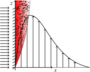
We consider a steady-state two-phase flow of dispersed bubbles as depicted in figure 1, and use a two-fluid formulation (Ishii & Hibiki Reference Ishii and Hibiki2011) to describe the average flow field and phase distribution along the vertical plate. Assuming no acceleration between liquid ( $l$) and gas ( $g$) phases, typically valid for bubbly flows, we adopt the mixture model (Taivassalo & Kallio Reference Taivassalo and Kallio1996; Ishii & Hibiki Reference Ishii and Hibiki2011). This model considers the gas–liquid mixture as a single fluid and includes additional closure relations for the unresolved flow features. The mixture density ( $\rho$) is the volume-averaged density of the liquid and gas phases, which in terms of the gas volume fraction ( $\varepsilon$) and liquid density ( $\rho _{l}$) reads
 \begin{equation} \rho = \rho_{{l}} (1-\varepsilon), \end{equation}
where we neglected the contribution of the gas phase to the mixture density due to its typically much lower density (i.e.  $\rho _{g} \ll \rho _{l}$). We then introduce the volume ( $\boldsymbol {U}$)- and mass ( $\boldsymbol {u}$)-averaged velocities
 $$\begin{gather} \boldsymbol{U} \equiv \boldsymbol{U}_{{l}} + \boldsymbol{U}_{{g}}, \end{gather}$$
 $$\begin{gather}\rho \boldsymbol{u} \equiv \rho_{{l}} \boldsymbol{U}_{{l}} + \rho_{{g}} \boldsymbol{U}_{{g}}, \end{gather}$$
where  $\boldsymbol {U}_{{l}} \equiv (1-\varepsilon )\boldsymbol {u}_{{l}}$ and $\boldsymbol {U}_{{g}} \equiv \varepsilon \boldsymbol {u}_{{g}}$ are the superficial liquid and gas velocities expressed in terms of the interstitial velocities $\boldsymbol {u}_{{l}}$ and $\boldsymbol {u}_{{g}}$. Note that introducing the mixture formulation amounts to averaging the governing equations over a sufficiently large space/time scale. However, the description of the multiphase flow system requires capturing subscale features (e.g. those related to the motion of bubbles with respect to the mixture) which need to be modelled instead via so-called closure models. This includes the superficial slip velocity,
 \begin{equation} \boldsymbol{U}_{{slip}} \equiv \boldsymbol{U}_{{g}} - \varepsilon \boldsymbol{U} = \varepsilon (\boldsymbol{u}_{{g}} - \boldsymbol{U} ), \end{equation}
which is sometimes referred to as the drift flux or slip flux. The slip velocity is the difference between the real flux of gas (i.e.  $\varepsilon \boldsymbol {u}_{{g}}$) and the flux predicted by the mixture (i.e. $\varepsilon \boldsymbol {U}$).

Figure 1. Schematic of the set-up for a gas-evolving vertical plate. Typical profiles of vertical velocity  $w$ and the gas-to-liquid volume ratio $\theta \propto \varepsilon /(1-\varepsilon )$ at an arbitrary location.
Since neither  $\boldsymbol {u}_{{g}}$ nor $\boldsymbol {u}_{{l}}$ is resolved, central to the mixture model are the semi-empirical relations that describe the slip velocities. Slip velocities result from the balance between drag and bubble forces, like lift, buoyancy or bubble–bubble interactions. Additional terms, such as bubble coalescence, break-up or turbulent interaction, are neglected in this study. In defining the slip velocities, we assume that the vertical buoyant rise velocity of bubbles relative to the liquid can be neglected with respect to the liquid velocity itself. In the horizontal direction, we neglect the lift forces and consider only the bubble–bubble interactions that lead to hydrodynamic dispersion:
 \begin{equation} \boldsymbol{U}_{{slip}}=-D_{eff}\boldsymbol{\nabla} \varepsilon, \end{equation}
where we introduce a new, effective, hydrodynamic dispersion coefficient:
 \begin{equation} D_{{eff}} = \frac{D_{{b}}}{(1-\varepsilon)^2},\end{equation}
which includes a  $1/( 1-\varepsilon )^{2}$ factor to approximately account for the additional repulsive effects that arise as the gas fraction increases. Details concerning the derivation of this particular form can be found in Appendix C. This can be seen as one of the mechanisms keeping volume fractions below $1$. For particle suspensions, this is often modelled by adding a ‘solid pressure’ (Johnson & Jackson Reference Johnson and Jackson1987), which mathematically has a similar effect.
The magnitude of the diffusivity is obtained by analogy with solid particle suspensions, which was found to be approximately given by the particle radius times the Stokes settling velocity (Ham & Homsy Reference Ham and Homsy1988; Nicolai et al. Reference Nicolai, Herzhaft, Hinch, Oger and Guazzelli1995), so
 \begin{equation} D_{{b}} = \frac{d_{{b}} w_{St}}{2},\end{equation}
with  $d_{{b}}$ the bubble diameter and $w_{St} = { g d_{{b}}^2}/{18\nu _{{l}}}$ the Stokes rise velocity in terms of the kinematic liquid viscosity $\nu _{{l}}=\mu _{{l}}/\rho _{{l}}$. Note that we replace here the bubble size distribution with a single representative bubble diameter.
While this form of the slip velocity expression is arguably the least validated assumption of our model, it does reduce to the correct empirically validated limit at low gas fractions and allows us to describe the essence of solid pressure effects in a simplified way. In addition, only this particular form allows for a self-similarity solution of the boundary layer equations, as is demonstrated in Appendix A. As shown in § 5, the predictions following from this assumption are in good agreement with experiments.
For flows developing a laminar boundary layer along a vertical plate, we modify the compressible version of Prandtl's boundary layer theory (Anderson Reference Anderson2006) to include gravity:
 $$\begin{gather} \partial_x ( \rho u ) + \partial_z ( \rho w )= 0 , \end{gather}$$
 $$\begin{gather}\rho u w_x + \rho w w_z = \partial_x (\mu w_x ) + ( \rho_{l} - \rho ) g , \end{gather}$$
 $$\begin{gather}\rho u \partial_x \frac{1}{\rho} + \rho w \partial_z \frac{1}{\rho} = \partial_x \left(\rho_{l}\frac{D_{{b}} }{1-\varepsilon} \partial_x \frac{1}{\rho} \right), \end{gather}$$
where  $u$ and $w$ are the components of $\boldsymbol {u}$ in the horizontal $x$ direction and vertical $z$ direction, respectively. Far away from the wall, where $(\rho _{{l}} - \rho )g=0$, a hydrostatic pressure gradient is assumed to cancel the gravitation force. Close to the wall, this term is positive, due to the upwards force that buoyancy exerts on the mixture. The gas transport equation (2.10) follows from taking the divergence of $u = U - U_{slip}/ (1-\varepsilon)$, $\boldsymbol {\nabla }\boldsymbol {\cdot}\boldsymbol {U}=0$ (since gas and liquid are conserved, i.e. $\boldsymbol {\nabla }\boldsymbol {\cdot}\boldsymbol {U}_{{g}}=\boldsymbol {\nabla }\boldsymbol {\cdot}\boldsymbol {U}_{{l}}=0$), inserting (2.1) and (2.5) and finally invoking $1/( 1-\varepsilon )^2 \partial _x \varepsilon = \partial _x ( 1 / ( 1-\varepsilon ) )$. Note that additional $\rho$ and $1/\rho$ terms are included in the convective term to render the final form in terms of the mass-averaged mixture velocity $(u,w)$ and the specific volume $1/\rho$.
The resulting equations (2.8)–(2.10) resemble those of high-speed aerodynamics, inspiring our solution approach. It is worth mentioning that the last equation corresponds to the conservation of the gas phase expressed in terms of specific volume ( $1/\rho$).
We assume the following rheological relation for mixture viscosity (Ishii & Zuber Reference Ishii and Zuber1979):
 \begin{equation} \mu = \frac{\mu_{{l}}}{1-\varepsilon}, \end{equation}
and define the following boundary conditions:
 $$\begin{align} u\rvert_{x=0} = w\rvert_{x=0} &= 0 , \lim_{x\to\infty}w = 0 , \end{align}$$
 $$\begin{align}\left.-\frac{D_{{b}}}{( 1-\varepsilon )^2} \frac{\partial \varepsilon}{\partial x}\right\vert_{x=0} &= U_{{w}} (1-\varepsilon_{{w}}) ,\quad \lim_{x\to \infty} \varepsilon = 0, \end{align}$$
which completes the formulation of the problem. The Neumann boundary condition for the gas fraction follows from (2.4) and (2.5), which give  $- ({D_{{b}}}/{( 1-\varepsilon )^{2}}) \boldsymbol {\nabla } \varepsilon = \boldsymbol {U}_{{g}}-\boldsymbol {U}\varepsilon$, and assuming $\boldsymbol {U}_{{l}}\approx 0$ owing to the very low specific volume of the liquid with respect to the gas phase. In typical electrochemical systems, the superficial gas velocity at the wall $U_{{w}} = j\mathcal {V}_{{m}}/n{F}$ can be related to the current density $j$, the number of gas molecules $n$ produced per electron converted in the reaction, Faraday's constant ${F}$ and the molar volume of the gas $\mathcal {V}_{m}$ – typically given by the ideal gas law as $\mathcal {V}_{{m}} = {R}T/p$, where ${R}$ is the ideal gas constant, $T$ the absolute temperature and $p$ the pressure.
3. Methodology
Next, we summarize the steps leading to the development of the self-similarity solution. The procedure is similar to that employed in obtaining a self-similar solution for high-speed compressible flows (Anderson Reference Anderson2006), with variations to include the dependency on gravity.
Stream function formulation. We first introduce a stream function  $\varPsi$ for the mass flux:
 \begin{equation} \rho u =-\varPsi_z , \quad \rho w = \varPsi_x, \end{equation}
which makes (2.8) automatically satisfied. We rewrite the other governing equations as
 $$\begin{gather} - \varPsi_z \partial_x \frac{\varPsi_x}{\rho} + \varPsi_x \partial_z \frac{\varPsi_x}{\rho} = \partial_x \left( \frac{\rho_{{l}}\mu_{{l}}}{\rho} \partial_x \frac{\varPsi_x}{\rho} \right) + ( \rho_{{l}}-\rho )g, \end{gather}$$
 $$\begin{gather}- \varPsi_z \partial_x \frac{1}{\rho} + \varPsi_x \partial_z \frac{1}{\rho} = \partial_x \left(D_{{b}}\frac{ \rho_{l}^2}{\rho} \partial_x \frac{1}{\rho} \right), \end{gather}$$
where subscripts  $x$ and $z$ denote partial derivatives.
Dorodnitsyn transformation. Now, we introduce the following self-similarity variable  $\eta$:
 \begin{equation} \eta = \frac{Ar_{*z}^{1/5}}{z}\int_0^x \frac{\rho}{\rho_{{l}}}\, {{\rm d}\kern0.06em x}', \end{equation}
where we introduce the modified Archimedes number  $Ar_{*z} = gU_{w}\,z^4/\nu _{l}^2 D_{b}$. This self-similarity transformation can be seen as combining the transformation proposed by Sparrow & Gregg (Reference Sparrow and Gregg1956) for Boussinesq flows developing along a vertical flat plate subject to constant heat flux with the original Dorodnitsyn transformation (Anderson Reference Anderson2006) for compressible flows. Note that in this particular type of transformation, the new coordinate $\eta$ explicitly depends on the vertical coordinate $z$, while the dependency on the horizontal $x$ coordinate is introduced via the density-weighted integral. The intent of such transformation is to simplify the calculation of $w$ in Prandtl's boundary layer equations. In particular,
 \begin{equation} w = \frac{\varPsi_x}{\rho} = \frac{\eta_x}{\rho}\varPsi_\eta = \frac{Ar_{*z}^{1/5}}{z \rho_{l}} \varPsi_\eta,\end{equation}
which removes the explicit dependency on  $\rho$ of the terms involving $w$, arguably simplifying the treatment of the boundary layer equations despite the variable density. Step-by-step details on the application of such transformation can be found in Appendix A.
Function transformation. Next, we adopt the following transformation for the unknowns  $\varPsi$ and $1/(1-\varepsilon )$ in terms of the self-similar functions $f(\eta )$ and $\theta (\eta )$:
 $$\begin{gather} \varPsi = \mu_{{l}} Ar_{*z}^{1/5} f(\eta), \end{gather}$$
 $$\begin{gather}\frac{1}{1-\varepsilon} = 1 +Pe_{{b}z} Ar_{*z}^{-1/5} \theta(\eta), \end{gather}$$
where we introduce the Péclet number  $Pe_{{b}z} = U_{w} z / D_{b}$. These transform equations (3.2) and (3.3) into the system
 $$\begin{gather} f''' = \frac{3}{5} \,f'^2 - \frac{4}{5}\, f\, f'' - \theta, \end{gather}$$
 $$\begin{gather}\theta'' = \frac{Pr_{{b}}}{5} (\,f'\theta - 4\, f\theta'), \end{gather}$$
where the bubble Prandtl number  $Pr_{{b}} = \nu _{{l}} / D_{{b}}$. The system is subject to the boundary conditions
 $$\begin{align} f\rvert_{\eta=0} = f'\rvert_{\eta=0} &=0 \quad \lim_{\eta\to \infty}f' =0, \end{align}$$
 $$\begin{align}\theta'\rvert_{\eta=0} &=-1 \lim_{\eta\to \infty}\theta =0, \end{align}$$
where a prime ( $'$) denotes a derivative with respect to $\eta$ to shorten the expressions. These transformations now allow us to derive a similarity solution. The system of (3.9) and (3.10) is the equivalent of the classical result for Boussinesq natural convection with constant heat flux (Sparrow & Gregg Reference Sparrow and Gregg1956). However, the most remarkable change is the shape of the buoyant scalar (i.e. $\varepsilon$). In particular, (2.10) gives
 \begin{equation} \varepsilon = \frac{Pe_{{b}z} Ar_{*z}^{-1/5}\theta}{1+Pe_{{b}z} Ar_{*z}^{-1/5}\theta}, \end{equation}
whereas in the thermal convection case (Sparrow & Gregg Reference Sparrow and Gregg1956)  $\varepsilon = Pe_{{b}z} Ar_{*z}^{-1/5}\theta$, which agrees with (3.12) when $Pe_{{b}z} Ar_{*z}^{-1/5}\theta {\ll 1}$. This is expected since for very low gas fractions, we should recover the Boussinesq hypothesis. The denominator in (3.12) ensures that the gas fraction does not exceed unity, a phenomenon in bubbly flow with no equivalent in thermal natural convection.
The vertical velocity field can be recovered from (3.5) and (3.6) as
 \begin{equation} w = \frac{\nu_{l}}{z} Ar_{*z}^{2/5} f', \end{equation}
which gives a scaling with height proportional to  $z^{3/5}$, equal to the thermal convection solution (Sparrow & Gregg Reference Sparrow and Gregg1956).
The mass flow rate per unit width [ ${\rm kg}\ {\rm m}^{-1}\ {\rm s}^{-1}$] is then equal to
 \begin{equation} \int_0^\infty \rho w \,{{\rm d}\kern0.06em x} = \int_0^\infty \varPsi_x \,{{\rm d}\kern0.06em x} = \varPsi_\infty = \mu_{{l}}Ar_{*z}^{1/5}f_\infty, \end{equation}
which scales with  $z^{4/5}$, accounting for the suction in the horizontal direction from outside the plume.
The wall shear stress  $\tau _{w}$ [Pa] is given by
 \begin{equation} \tau_{w} \equiv \left. { \mu \frac{\partial w}{\partial x}}\right\vert_{w} = \mu_{l} \frac{\nu_{l}}{z^2} Ar_{*z}^{3/5} f''_{w}, \end{equation}
where we used (2.11) for the mixture viscosity  $\mu = {\mu _{{l}}}/({1- \varepsilon })$ as well as (2.1), (3.4) and (3.13).
The wall shear stress shows the same scaling with height and current density irrespective of the local gas fraction, as in the Boussinesq hypothesis case (Sparrow & Gregg Reference Sparrow and Gregg1956). This is due to the variations of  $\mu$ and $\rho$ with $\varepsilon$ cancelling each other. However, the wall shear rate $w'_{{w}} = {\tau _{{w}} }/{ \mu } = ({\tau _{{w}} }/{ \mu _{{l}}}) ( 1- \varepsilon _{{w}} )$ [s $^{-1}$] does show a transition between $z^{2/5}$ and $z^{3/5}$. Using (3.12) this gives
 \begin{equation} w'_{{w}} = \frac{\nu_{l}}{z^2} \frac{f''_{w} Ar_{*z}^{3/5}}{1+Pe_{{b}z} Ar_{*z}^{-1/5}\theta_{{w}}}. \end{equation}
Finally, we may define the dimensionless gas plume thickness as  ${\delta _{{g}}}/{z} = - ({z^{-1}}/\eta_x) ({\theta _{{w}} }/{\theta '_{{w}} })$. It follows from the boundary conditions in (3.11) and (3.4) and (2.1) that
 \begin{equation} \frac{\delta_{{g}}}{z} = Ar_{*z}^{-1/5} ( 1 + Pe_{{b}z}Ar_{*z}^{-1/5} \theta_{{w}} )\theta_{{w}}, \end{equation}
which shows a transitional scaling between  $z^{-4/5}$ and $z^{-3/5}$. Note, however, that as $z \to \infty$, the model loses accuracy as turbulence may set in.
4. Results
The final system of (3.8)–(3.11) can be solved by numerical integration for different values of  $Pr_{{b}}$, which we choose corresponding to a wide range of bubble diameters.
The numerical method consists of a classical shooting algorithm, which adjusts the value for  $\theta$ at $\eta =0$ iteratively until the boundary conditions are satisfied. The domain of integration ranges from $\eta =0$ to $\eta = 50$. This range was chosen such that parameters in the vicinity of the wall do not change substantially upon a further increase. For $f_\infty$, convergence was achieved for a substantially larger domain up to $\eta =800$. Results for $f'$ and $\theta$ are shown in figure 2. Through (3.12) and (3.13) these dimensionless quantities are related to the gas fraction $\varepsilon$ and the vertical velocity $w$, respectively.


From these profiles, we can obtain relevant parameters such as wall gas fraction  $\varepsilon _{w}$ and wall shear stress $\tau _{w}$, which depend on $\theta _{w}$ and $f''_{w}$; and also on vertical mass flow rate, which depends on $f_\infty$. Values of $\theta _{w}$, $f''_{w}$ and $f_\infty$ are reported in figure 3 for different $Pr_{{b}}$ numbers. All profiles show a transition at $Pr_{{b}}\approx 1$, corresponding to the switch in the predominance of the momentum diffusivity $\nu$ over the bubble diffusivity $D_{{b}}$. For convenience, figure 3 has as an additional axis showing typical bubble sizes assuming Stokes drag and an aqueous-like viscosity. Results show different asymptotic behaviours for small bubbles ( $d_{{b}}<100\ {\rm \mu}\textrm {m}$, typical for electrolytic bubbles) and larger bubbles ( $d_{{b}}>100\ \mathrm {\mu }\textrm {m}$, typical for bubbles due to boiling). A power-law scaling is obtained for the two regions, shown in the figure, resulting in approximate asymptotic relations for both parameters:

Figure 3. The wall values  $\theta _{w}$ and $f''_{{w}}$ and $f_{\infty }$ as a function of the bubble Prandtl number $Pr_{{b}} = \nu / D_{{b}}$. The upper $x$ axis shows the corresponding bubble diameter using (2.7), assuming typical values of $g=9.81\ {\rm m}\ {\rm s}^{-2}$ and $\nu _{{l}}=10^{-6}\ {\rm m}^2\ {\rm s}^{-1}$. We note that for bubbles with $d_{{b}} \gtrsim 100\ \mathrm {\mu }$m, $w_{{St}}$ used in (2.7) no longer corresponds to the buoyant slip velocity as Stokes drag becomes invalid.
 $$\begin{gather} \theta_{w} \approx \begin{cases} 1.63Pr_{{b}}^{-1/5} & Pr_{{b}} \gtrsim 1 \\ 1.63 Pr_{{b}}^{-1/3} & Pr_{{b}} \lesssim 1, \end{cases} \end{gather}$$
 $$\begin{gather}f''_{w} \approx \begin{cases} 1.50Pr_{{b}}^{-2/5} & Pr_{{b}} \gtrsim 1 \\ 1.50 Pr_{{b}}^{-1/3} & Pr_{{b}} \lesssim 1, \end{cases} \end{gather}$$
 $$\begin{gather}f_\infty \approx \begin{cases} 1.40Pr_{{b}}^{-3/5} & Pr_{{b}} \gtrsim 1 \\ 1.25 Pr_{{b}}^{-3/10} & Pr_{{b}} \lesssim 1. \end{cases} \end{gather}$$
Approximations combining both asymptotic limits can be found in Appendix A. These values can be used to approximate wall gas fraction  $\varepsilon _{w}$, wall shear stress $\tau _{w}$ and wall shear rate $w'_{{w}}$ through (3.12), (3.15) and (3.16), respectively, to give
 $$\begin{gather} \frac{ \varepsilon_{w} }{1 - \varepsilon_{w}} \approx 1.63 \times \begin{cases} \left( \dfrac{ \nu_{l} U_{{w}}^4\, z }{g D_{b}^3 } \right)^{1/5} & d_{{b}}\lesssim 100 \ \mathrm{\mu}\textrm{m} \\ \left( \dfrac{\nu_{l}^{1/3} U_{{w}}^4\, z}{g D_{b}^{7/3} } \right)^{1/5} & d_{{b}}\gtrsim 100\ \mathrm{\mu}\textrm{m}, \end{cases} \end{gather}$$
 $$\begin{gather}\tau_{w} \approx 1.5 \rho_{{l}} \times \begin{cases} \left( \dfrac{g^3 \nu_{l}^2 U_{w}^3\, z^2 }{ D_{{b}} }\right)^{{1}/{5}} & d_{{b}}\lesssim100\ \mathrm{\mu}\textrm{m} \\ ( g^3 (\nu_{l}^{7}/D_{{b}}^{4} )^{{1}/{3}} U_{w}^3\, z^2 )^{{1}/{5}} & d_{{b}}\gtrsim100\ \mathrm{\mu}\textrm{m} \\ \end{cases} \end{gather}$$
and
 \begin{equation} w'_{w} \approx 1.5\times \begin{cases} \dfrac{ \left( \dfrac{g^3 U_{w}^3\, z^2 }{ D_{{b}} \nu_{l}^3 }\right)^{1/5} }{1+1.63 \left( \dfrac{ \nu_{l} U_{{w}}^4\, z }{g D_{b}^3 } \right)^{1/5} } & d_{{b}}\lesssim100\ \mathrm{\mu}\textrm{m} \\ \dfrac{\left( \dfrac{ g^3 U_{w}^3\, z^2 }{ (\nu_{l}^{8} D_{{b}}^{4} )^{{1}/{3}} } \right)^{1/5}}{1+1.63 \left( \dfrac{\nu_{l}^{1/3} U_{{w}}^4\, z }{g D_{b}^{7/3} } \right)^{1/5} } & d_{{b}}\gtrsim100 \ \mathrm{\mu}\textrm{m}. \end{cases} \end{equation}
This last relation shows a transition from a proportionality with  $U_{{w}}^{3/5}z^{2/5}$ at low wall gas fractions to $U_{{w}}^{-1/5}z^{1/5}$ at wall gas fractions close to one. Interestingly, the viscosity increases faster with increasing $U_{{w}}$ than the wall shear stress, resulting in a decreasing wall shear rate with increasing gas flux in this regime. This limiting result strongly depends on the exact relation between effective viscosity and gas fraction, i.e. (2.11), and the assumed maximum gas fraction of unity.
The mass flux per unit width, from (3.14), reads
 \begin{equation} \int_0^\infty \rho w \,{{\rm d}\kern0.06em x} = \begin{cases} 1.4\rho_{{l}} ( g D_{b}^2 U_{w}\,z^4 )^{1/5} & d_{{b}}\lesssim100 \ \mathrm{\mu}\textrm{m} \\ 1.25\rho_{{l}} ( g \nu_{l}^{3/2} D_{b}^{1/2} U_{w}\,z^4)^{1/5} & d_{{b}}\gtrsim 100 \ \mathrm{\mu}\textrm{m}. \end{cases} \end{equation}
This shows an almost linear increase with  $z$ and a much weaker dependence on the wall gas flux $U_{{w}}$. Rajora & Haverkort (Reference Rajora and Haverkort2023) found a linear dependence on both $z$ and $U_{{w}}$, for a plume in the shape of a step function. When $Pe_{{b}z} Ar_{*z}^{-1/5} \gg 1$ we have $\varepsilon _{{w}}\approx 1$ and the gas plume described by (3.12) similarly becomes a smoothed step function. However, in this limit, there is no liquid inside the plateau region of the gas plume and the analysis of Rajora & Haverkort (Reference Rajora and Haverkort2023) fails in this case.
Finally, using (3.17), (4.1) and (4.4) the gas plume thickness becomes
 \begin{equation} \delta_{{g}} \approx 1.63 \left(\frac{z}{ g U_{w} } \right)^{{1}/{5}} \times \begin{cases} \nu_{l}^{{1}/{5}} D_{b}^{{2}/{5}}\left( 1+\left( \frac{ \nu_{l} U_{{w}}^4\, z }{g D_{b}^3 } \right)^{1/5} \right) & d_{{b}}\lesssim100\ \mathrm{\mu}\textrm{m} \\ \nu_{l}^{{1}/{15}} D_{b}^{{8}/{15}}\left( 1+ \left( \frac{\nu_{l}^{1/3} U_{{w}}^4\, z }{g D_{b}^{7/3} } \right)^{1/5} \right) & d_{{b}}\gtrsim100 \ \mathrm{\mu}\textrm{m}. \end{cases} \end{equation}
This shows a transition from a proportionality with  $(z / U_{{w}} )^{1/5}$ at low gas fraction to a proportionality with $U_{{w}}^{3/5}z^{2/5}$ at high wall gas fractions. The latter positive dependence on gas flux is in agreement with most experimental findings in which the plume thickness increases with increasing current density. A similar transition was found by Rajora & Haverkort (Reference Rajora and Haverkort2023) using approximate methods, where at high gas fractions, depending on $Pr_{{b}}$, a proportionality of between $( U_{{w}}z)^{1/3}$ and $U_{{w}}^{0.73}z^{0.43}$ was obtained. The result obtained here is virtually exact, valid for all wall gas fractions, and arguably more elegant.
5. Validation
Here we compare our results with experimental data for gas-evolving electrodes. Two different sets of experiments are considered: wall shear stress measurements of Hiraoka et al. (Reference Hiraoka, Yamada, Mori, Sugimoto, Hakushi, Matsuura and Nakamura1986) and gas plume thickness data of Fukunaka et al. (Reference Fukunaka, Suzuki, Ueda and Kondo1989). Both datasets concern hydrogen-evolving electrodes.
The experiments of Hiraoka et al. (Reference Hiraoka, Yamada, Mori, Sugimoto, Hakushi, Matsuura and Nakamura1986) report direct measurements of the average wall shear stress. Their set-up consisted of a planar vertical working electrode immersed in a KOH solution between two counter electrodes. The measured weight of the working electrode was recorded against the current density and subtracted from the weight that was measured when no gas evolution was present. This measurement allowed to determine  $\tau _{w}$.
A comparison with our model predictions is shown in figure 4. We averaged wall shear stress for (3.15) as
 \begin{equation} \langle {\tau_w} \rangle = \frac{1}{h}\int_0^h \tau_w\, {\rm d}z = \frac{5}{7} \tau_w \vert_h. \end{equation}
Figure 4. Experimental values of the wall shear stress  $\tau _{{w}}$ as a function of the gas-evolving velocity $U_{w}$. The corresponding current density for H $_2$ evolution is reported on the top $x$ axis. Data taken from Fukunaka et al. (Reference Fukunaka, Suzuki, Ueda and Kondo1989). Bubble diameter is set to $d_{{b}} = 200\ \mathrm {\mu }\textrm {m}$.
The average wall shear stress at the electrode surface for electrodes of different heights in the range of  $h \in [4\unicode{x2013}10]\ \textrm {cm}$ is shown. The predicted results are overall in good agreement with the experimental data except for very low gas-evolving velocities (i.e. low current densities).
The gas plume thickness is compared with the experimental data of Fukunaka et al. (Reference Fukunaka, Suzuki, Ueda and Kondo1989). Their experimental set-up consists of a segmented working electrode immersed in a transparent beaker with 0.05 M CuSO $_4$–1.85 M H $_2$SO $_4$ solution and a single counter electrode. The gas plume thickness was measured from pictures taken from the side of the beaker. The bubble detachment diameter was found to be in the range $d_{{b}} \in [60\unicode{x2013}200]\ \mathrm {\mu }\textrm {m}$.
The experimental data of the gas plume thickness are compared with our model predictions in figure 5. The bubble diameter,  $d_{b}$, was used as a fitting parameter, which provided results within the observed range. The obtained increase in bubble size with increasing current density is in good agreement with the data reported for H $_2$SO $_4$ by Janssen & Hoogland (Reference Janssen and Hoogland1973). Figure 5 includes a comparison of the present theory with the Boussinesq hypotheses using a corresponding bubble diameter of $d_{{b,B}}$ (see figure 5). Our result shows a slope that is marginally closer to that of the data, but both results can explain the data reasonably well and with reasonable bubble diameters. The reason is that not even a decade of different heights is included in the data, and (4.8) depends rather weakly on height.

Figure 5. Experimental values of the gas plume thickness  $\delta _{g}$ as a function of height h for the new model (solid line) and with the classical Boussinesq assumption (dashed line). Data taken from Hiraoka et al. (Reference Hiraoka, Yamada, Mori, Sugimoto, Hakushi, Matsuura and Nakamura1986).
A much larger difference between the predictions of the present model and the Boussinesq approximation was found for the mass transfer coefficient, as recently reported in Valle & Haverkort (Reference Valle and Haverkort2024) and Haverkort (Reference Haverkort2024b). The reason is that the mass transfer coefficient is strongly dependent on the shear at the wall  $w'$, which shows a much more acute difference. Here, the predictions from the present model are in much better agreement with the data than those of the Boussinesq approximation.
6. Conclusion
We have developed a new self-similarity solution for laminar bubbly flow evolving from a vertical plate, which considers variable density, viscosity and hydrodynamic dispersion, all depending on the local gas fraction. Results for both small and large bubbles produce simple power-law relations for the wall shear stress and the gas fraction at the wall, which are critical parameters in process technology. The wall strain rate and gas plume thickness show a transition between low to moderate gas fractions and gas fractions near one.
The new results go beyond the classical Boussinesq theory, which is only valid for very low gas fractions. Owing to the strong dependence of density and viscosity with gas fraction, the new results expand the validity of this analysis to general void fractions, as far as the flow remains laminar.
Our theoretical analysis reveals that a self-similarity solution is only possible if the bubble diffusivity is proportional to  $(1-\varepsilon )^{-2}$, which is equivalent to formulating the gas fraction convection–diffusion equation in terms of specific volumes and using a constant diffusivity. While this is a convenient assumption that allows for a neat analytical treatment, it can also be physically motivated to approximately model increased diffusion at high gas fractions, preventing the system from reaching non-physical gas fractions $\varepsilon > 1$.
By introducing a novel change of coordinates and variables we observe that the solutions show an asymptotic transition between the classical Boussinesq result for relatively low gas flow rates and short heights and a new asymptotic solution for which the wall gas fraction tends to one.
Comparison with experimental results shows good agreement with existing experimental literature data for wall shear stress and bubble plume thickness. Considering the simplified nature of the model and the number of assumptions made, the agreement in the observed trends is highly satisfactory.
Further work in this area requires an improvement of the closure models for hydrodynamic dispersion of bubbles. An immediate step would be to perform a linear stability analysis of the base flow presented above.
Funding
We acknowledge the Dutch Research Council (NWO) for funding under grant agreement KICH1.ED04.20.011.
Declaration of interest
The authors report no conflict of interest.
Appendix A. Derivation of the self-similar solution
Here, we reproduce the analytical treatment that leads to our self-similar solution in more detail. The following exposition is inspired by that presented in Anderson (Reference Anderson2006), but adapted to the presence of gravity as the driving force of the system and our particular dependence of diffusivity and viscosity on gas fraction.
Constitutive equations. The mixture model (Ishii & Hibiki Reference Ishii and Hibiki2011) requires defining the slip velocities  $\boldsymbol {U}_{{slip}}$, which accounts for the relative velocity between the gas phase and the mixture. We assume the following form:
 \begin{equation} \boldsymbol{U}_{{slip}}=\boldsymbol{U}_{{Hd}}=- \frac{D_{{b}}}{( 1-\varepsilon )^{2}} \boldsymbol{\nabla} \varepsilon =- D_{{b}} \boldsymbol{\nabla} \frac{1}{1-\varepsilon}, \end{equation}
which produces a high diffusivity when  $\varepsilon \to 1$, accounting for the nonlinear effects arising from bubble crowding.
Governing equations. The governing equations consist of the mixture model equations:
 $$\begin{align} \partial_x ( \rho u ) + \partial_z ( \rho w )&= 0 , \end{align}$$
 $$\begin{align}\rho u w_x + \rho w w_z &= \partial_x (\mu w_x ) + ( \rho_{l} - \rho ) g , \end{align}$$
 $$\begin{align}\rho u \partial_x \frac{1}{\rho} + \rho w \partial_z \frac{1}{\rho} &= \partial_x \left(\rho_{l}\frac{D_{{b}} }{1-\varepsilon} \partial_x \frac{1}{\rho} \right), \end{align}$$
and the boundary conditions
 $$\begin{align} u\rvert_{x=0} = w\rvert_{x=0} &= 0 , \quad\quad\quad\quad\quad\, \lim_{x\to\infty}w = 0 , \end{align}$$
 $$\begin{align}\left.-\dfrac{D_{{b}}}{( 1-\varepsilon )^2} \frac{\partial \varepsilon}{\partial x}\right\vert_{x=0} &= U_{{w}} (1-\varepsilon_{{w}}) ,\quad \lim_{x\to \infty} \varepsilon = 0. \end{align}$$
 Stream function formulation. We first introduce a stream function  $\varPsi$ for the mass flux:
 \begin{equation} \rho u =-\varPsi_z , \quad \rho w = \varPsi_x, \end{equation}
which makes (A2) automatically satisfied. We rewrite the other governing equations as
 $$\begin{align} - \varPsi_z \partial_x \frac{\varPsi_x}{\rho} + \varPsi_x \partial_z \frac{\varPsi_x}{\rho} &= \partial_x \left( \frac{\rho_{{l}}\mu_{{l}}}{\rho} \partial_x \frac{\varPsi_x}{\rho} \right) + ( \rho_{{l}}-\rho )g, \end{align}$$
 $$\begin{align}- \varPsi_z \partial_x \frac{1}{\rho} + \varPsi_x \partial_z \frac{1}{\rho} &= \partial_x \left(D_{{b}}\frac{ \rho_{l}^2}{\rho} \partial_x \frac{1}{\rho} \right), \end{align}$$
where subscripts  $x$ and $z$ denote partial derivatives.
Dorodnitsyn transformation. We transform the  $(x,z)$ coordinate system into dimensionless $(\eta, z)$ coordinates, which have the following structure:
 \begin{equation} \eta = a(z) \int_{0}^{x} {\rho}\, {{\rm d}\kern0.06em x}', \end{equation}
where  $a(z)$ is a function to be determined. The differential $\partial _x$ in terms of $\eta$ then reads
 \begin{equation} \partial_x = \eta_x \partial_\eta \hphantom{ + z_x \partial_z} = a \rho \partial_\eta,\end{equation}
where note that we have suppressed showing the dependence of  $a$ on $z$ to simplify the notation. The aforementioned change of coordinates allows us to reformulate equations (A8) and (A9) in terms of $\eta$ and $z$:
$z$:
 \begin{align} - a^2 \varPsi_z \varPsi_{\eta \eta} + a \varPsi_\eta \partial_z ( a \varPsi_\eta ) &= a^3 \mu_{l} \rho_{l} \varPsi_{\eta \eta \eta} + \frac{\varepsilon}{1-\varepsilon}g, \end{align}
 \begin{align}- \varPsi_z \partial_\eta \frac{1}{1-\varepsilon} + \varPsi_\eta \partial_z \frac{1}{1-\varepsilon} &= D_{{b}}\rho_{{l}} \partial_{\eta\eta} \frac{1}{1-\varepsilon}, \end{align}
and the boundary conditions:
 $$\begin{align} -\left. \frac{\varPsi_z}{\rho} \right\vert_{\eta=0} = \left.\frac{\varPsi_x}{\rho} \right\vert_{\eta=0} &= 0 , \quad \lim_{\eta \to \infty} \frac{\varPsi_x}{\rho} = 0, \end{align}$$
 $$\begin{align}\left.\frac{D_{{b}} \rho_{l}}{U_{w}} a \partial_\eta \frac{1}{1-\varepsilon} \right\vert_{\eta=0} &=-1 , \quad \lim_{\eta \to \infty} \varepsilon = 0. \end{align}$$
 Separation of variables. The next step is to attempt a prototype for  $\varPsi$ and $1/(1-\varepsilon )$ in terms of functions of $z$ and $\eta$:
 \begin{equation} \varPsi = k(z) f(\eta), \quad \frac{1}{1-\varepsilon} = 1 + b(z) \theta(\eta). \end{equation}
Substituting these equations into (A12) and (A13), we obtain
 $$\begin{align} - a^2 k k_z f\, f_{\eta\eta} + a k ( a_z k + a k_z ) f^2_\eta &= a^3 k\mu_{l}\rho_{l}f_{\eta\eta\eta} + b \theta g, \end{align}$$
 $$\begin{align}k b_z f_\eta \theta - k_z b f \theta_\eta &= D_{{b}} \rho^2_{l} a b \theta_{\eta \eta}, \end{align}$$
and the boundary conditions (A14a,b) and (A15a,b):
 $$\begin{align} f \rvert_{\eta=0} = f' \rvert_{\eta=0} &= 0 , \quad\ \ \, \lim_{\eta \to \infty} f' =0, \end{align}$$
 $$\begin{align}\left.\frac{D_{{b}} \rho_{l}}{U_{w}} a b \theta_\eta \right\vert_{\eta=0} &=-1 , \quad \lim_{\eta \to \infty} \theta = 0. \end{align}$$
Since the objective of the similarity analysis is to remove the dependency on  $z$ in the governing system of equations to formulate a system of similarity equations which is a function of $\eta$ only, we need to cancel the terms on $z$. To this aim, we attempt polynomial prototypes for $a$,
$a$,  $k$ and $b$ as $a = a_0 z^m$, $k= k_0 z^n$ and $b = b_0 z^o$, which transform equations (A17) and (A18) into
 $$\begin{align} a^2_0 k^2_0 z^{2m+2n-1} (( m+n ) f^2_\eta - n f\, f_{\eta\eta} ) &= \mu_{l} \rho_{l} a^3_0 k_0 z^{3m+n} f_{\eta\eta\eta} + g b_0 z^o \theta, \end{align}$$
 $$\begin{align}k_0 b_0 z^{n+o-1} ( o f_\eta \theta - n f \theta_\eta ) &= D_{{b}} \rho^2_{l} a_0 b_0 z^{m+o} \theta_{\eta \eta}. \end{align}$$
Together with the boundary conditions:
 $$\begin{align} f \rvert_{\eta=0} = f' \rvert_{\eta=0} &= 0 , \quad\ \ \, \lim_{\eta \to \infty} f' = 0, \end{align}$$
 $$\begin{align}\left.\frac{D_{{b}}}{U_{w}} \rho_{l} a_0 b_0 z^{m+o} \theta_\eta \right\vert_{\eta=0} &=-1 , \quad \lim_{\eta \to \infty} \theta = 0. \end{align}$$
 Grouping the terms in  $z$ imposes the following system of equations for compatibility:
 $$\begin{align} 2m+2n-1 &= o, \end{align}$$
 $$\begin{align}3m+n &= o, \end{align}$$
 $$\begin{align}n+o-1 &= m+o, \end{align}$$
 $$\begin{align}m+o &= 0. \end{align}$$
From these equations it can be checked that this is a redundant system (e.g. (A25a)–(A25b)  $=$ (A25c)) which has a non-trivial solution $m=-1/5$, $n=4/5$ and $o=1/5$. Attempting different exponents for $( 1-\varepsilon )$ in (A1) reveals that the system is incompatible unless the $( 1-\varepsilon )^{2}$ factor is used to modify the bubble diffusivity.
Once the result is obtained we can substitute back in (A21)–(A24a,b) to obtain, after rearranging,
 $$\begin{align} \frac{3}{5} f^2_\eta -
\frac{4}{5} f_{\eta\eta} &= \boxed{\frac{\mu_{l} \rho_{l}
a_0}{ k_0}}\ f_{\eta\eta\eta} + \boxed{\frac{g b_0}{ a^2_0
k^2_0}} \theta, \end{align}$$
$$\begin{align} \frac{3}{5} f^2_\eta -
\frac{4}{5} f_{\eta\eta} &= \boxed{\frac{\mu_{l} \rho_{l}
a_0}{ k_0}}\ f_{\eta\eta\eta} + \boxed{\frac{g b_0}{ a^2_0
k^2_0}} \theta, \end{align}$$
 $$\begin{align}\frac{1}{5} f_\eta \theta - \frac{4}{5} f \theta_\eta &= \boxed{\frac{\mu_{l} \rho_{l} a_0}{ k_0}} \frac{D_{l}}{\nu_{l}} \theta_{\eta \eta}. \end{align}$$
Here we have identified the bubble Prandtl number  $Pr_{{b}} = {\nu _{l}}/{D_{b}}$:
 $$\begin{align} f \rvert_{\eta=0} = f' \rvert_{\eta=0} &= 0 , \quad\ \ \, \lim_{\eta \to \infty} f' = 0, \end{align}$$
 $$\begin{align}\left. \boxed{\frac{D_{{b}}}{U_{w}} \rho_{l} a_0 b_0} \theta_\eta \right\vert_{\eta=0} &=-1 , \quad \lim_{\eta \to \infty} \theta = 0. \end{align}$$
We will adjust the coefficients  $a_0$, $k_0$ and $b_0$ to simplify the shape of the equations, making the boxed terms simplify to the arbitrary value of $1$:
$1$:
 $$\begin{align} \frac{\mu_{l} \rho_{l} a_0}{ k_0} &= 1, \end{align}$$
 $$\begin{align}\frac{g b_0}{ a^2_0 k^2_0} &= 1, \end{align}$$
 $$\begin{align}\frac{D_{{b}} \rho_{l} a_0 b_0}{U_{w}} &= 1. \end{align}$$
From this we obtain
 $$\begin{align} a_0 &= \frac{1}{z \rho_{l}} (Ar_{*z})^{1/5}, \end{align}$$
 $$\begin{align}k_0 &= \mu_{l} (Ar_{*z})^{1/5} , \end{align}$$
 $$\begin{align}b_0 &= Pe_{{b}z} (Ar_{*z})^{-1/5}. \end{align}$$
Here we have introduced the modified local Archimedes number  $Ar_{*z} = {{g U_{w} z^4}/{\nu _{l}^2 D_{b}}}$ and local bubble Péclet number as $Pe_{{b}z}= U_{w}z/D_{b}$. Substituting, we finally obtain
 \begin{align} \eta &= \frac{(Ar_{*z})^{1/5}}{z}\int^x_0 \frac{\rho}{\rho_{l}}\,{{\rm d}\kern0.06em x}', \end{align}
 \begin{align}\varPsi &= \mu_{l} (Ar_{*z})^{1/5} f(\eta), \end{align}
 \begin{align}\frac{1}{1-\varepsilon} &=1 + Pe_{{b}z} ( Ar_{*z})^{-1/5}\theta(\eta). \end{align}
Appendix B. All- $Pr_{{b}}$ fit of $\theta _{{w}}$, $f''_{{w}}$ and $f_{\infty }$


The asymptotic for fit for  $\theta _{{w}}$, $f''_{{w}}$ and $f_{\infty }$ is provided in the main text for the two limiting cases of $Pr_{{b}} \lesssim 1$ and $Pr_{{b}} \gtrsim 1$. However, it is worth including a general relation that converges to the right limits and that considers all $Pr_{{b}}$ ranges:
 $$\begin{gather} \theta_{w} \approx 1.63 (Pr_{{b}}^{-5.63/5} Pr_{{b}} + Pr_{{b}}^{-5.63/3} )^{1/5.63}, \end{gather}$$
 $$\begin{gather}f''_{w} \approx 1.50 (Pr_{{b}}^{25.72/5} Pr_{{b}} + Pr_{{b}}^{12.86/3} )^{-1/12.86}, \end{gather}$$
 $$\begin{gather}f_\infty \approx ( 1.40^4 Pr_{{b}}^{-12/5} Pr_{{b}} + 1.25^4 Pr_{{b}}^{-12/10} )^{1/4}. \end{gather}$$
For the range  $10^3 \lesssim d_{{b}} \lesssim 1\ \mathrm {\mu }\textrm {m}$ (which corresponds approximately to $4 \times 10^{-1} \lesssim Pr_b \lesssim 3 \times 10^6$), the maximum relative errors in these fits for $\theta _{{w}}$, $f''_{{w}}$ and $f_{\infty }$ compared with the actual computed values are $2.95\,\%$, $4.57\,\%$ and $2.06\,\%$, respectively.
Appendix C. Subscale model for hydrodynamic dispersion
At low concentrations, solid particles diffuse away from each other (Ham & Homsy Reference Ham and Homsy1988; Nicolai et al. Reference Nicolai, Herzhaft, Hinch, Oger and Guazzelli1995) with a diffusion coefficient given by (2.7). In confined systems, like those typically studied in settling, the Stokes velocity decreases with increasing dispersed phase fraction, which can be described by a hindrance function (Richardson & Zaki Reference Richardson and Zaki1954). However, due to clustering effects, bubbles rising in bubble columns tend to show the opposite behaviour of an increasing slip velocity with increasing high gas fraction (Simonnet et al. Reference Simonnet, Gentric, Olmos and Midoux2007). Electrolytically generated bubbles are typically much smaller than those in bubble columns, but were equally reported to show an increase in rise velocity with increasing gas fraction (Kreysa & Kuhn Reference Kreysa and Kuhn1985; Vogt Reference Vogt1987; Kellermann, Jüttner & Kreysa Reference Kellermann, Jüttner and Kreysa1998). Therefore, we opt not to include hindrance. However, we do want to consider the increase in dispersion that is known to take place for solids at high dispersed phase fractions.
At high concentrations point-contacts and collisions between solid particles cause repulsive inter-particle forces. We assume that a similar solid pressure mechanism is present in the case of bubbles, which contributes to pushing bubbles away from high-concentration regions and thus prevents high void fractions. This is typically modelled by including an additional stress term to the momentum equation of the dispersed phase. Several models have been suggested for it, most prominently is the addition of a solid pressure of the form (Johnson, Nott & Jackson Reference Johnson, Nott and Jackson1990)
 \begin{equation} p_{s} = \gamma_0 \rho g d \frac{( \varepsilon - \varepsilon_{min} )^{\gamma_1}}{( \varepsilon_{max} - \varepsilon )^{\gamma_2}}.\end{equation}
 In the context of the mixture model we equal each force acting on the dispersed phase to drag to obtain the corresponding slip velocity. Assuming Stokes flow,  $u_{Sp} \varepsilon 18\mu /d_{b}^2 = \boldsymbol {\nabla } p_s$ and thus
 \begin{equation} u_{Sp} =-\frac{d_{b}^2\boldsymbol{\nabla} p_{s}}{18 \mu \varepsilon} =-\gamma_0 w_{St}d_{b} \frac{ (\varepsilon-\varepsilon_{min} )^{\gamma_1}}{( \varepsilon_{max} - \varepsilon )^{\gamma_2}} \left( \frac{\gamma_1}{\varepsilon-\varepsilon_{min}} + \frac{\gamma_2}{\varepsilon_{max}-\varepsilon} \right) \frac{\boldsymbol{\nabla} \varepsilon }{\varepsilon} .\end{equation}
Now, substituting  $u_{Sp}$, (2.4) and (2.5) can be rewritten as
 \begin{equation} U_{slip} = \varepsilon ( 1-\varepsilon ) u_{slip} =- D_{eff} \boldsymbol{\nabla} \varepsilon.\end{equation}
Comparing with (C2), the hydrodynamic dispersion coefficient  $D_{Sp}$ becomes
 \begin{equation} D_{Sp} = 2\gamma_0 D_{b}( 1-\varepsilon ) \frac{ (\varepsilon-\varepsilon_{min} )^{\gamma_1}}{( \varepsilon_{max} - \varepsilon )^{\gamma_2}} \left( \frac{\gamma_1}{\varepsilon-\varepsilon_{min}} + \frac{\gamma_2}{\varepsilon_{max}-\varepsilon} \right).\end{equation}
In the literature several values have been proposed for the free parameters in this model including  $\varepsilon _{min}=0$, $\varepsilon _{max}=1$, $\gamma _0=1.75\times 10^{-3}$, $\gamma _1=2$ and $\gamma _2=5$ in Johnson et al. (Reference Johnson, Nott and Jackson1990) and $\varepsilon _{min}=0$, $\varepsilon _{max}=1$, $\gamma _0=5$, $\gamma _1=1$ and $\gamma _2=1$ in Josserand, Lagrée & Lhuillier (Reference Josserand, Lagrée and Lhuillier2006). Considering the large spread in these parameters in the literature, we propose to use the simplified form $D_{eff} = D_{b}(1-\varepsilon )^{-2}$ as given in (2.6). Note that this corresponds to setting $\gamma _0=1/4$, $\gamma _1 = 0$, $\gamma _2 = 2$ and $\varepsilon _{max}=1$ in (C4), so that hydrodynamic dispersion follows as a low gas fraction limit of the effect of solid pressure. Since for other choices of parameters or solid pressure models this is not the case, we add hydrodynamic diffusion to obtain $D_{eff} = D_{Hd} + D_{Sp}$ for these other models. A comparison for the resulting total dispersion coefficient as a function of gas fraction is plotted in figure 6. It may be seen that our expression is somewhat in between the values of other models used in the literature. Considering the scatter of data in the literature, and the trade-off between physical reliability and mathematical simplicity, we introduce the aforementioned effective bubble dispersion coefficient as a reasonable approximation of the models presented so far.

Figure 6. Comparison of our proposed effective bubble dispersion coefficient  $D_{eff}={1}/{( 1- \varepsilon )^2}$ with the combined hydrodynamic dispersion of Nicolai et al. (Reference Nicolai, Herzhaft, Hinch, Oger and Guazzelli1995) and solid pressure models of several authors (Johnson et al. Reference Johnson, Nott and Jackson1990; Josserand et al. Reference Josserand, Lagrée and Lhuillier2006). We have set $\varepsilon _{min}=0$ and $\varepsilon _{max}=1$.


 Open access