1. INTRODUCTION
The Earth Orientation Parameters (EOP): Length-Of-Day (LOD); xp, yp, pole coordinates and d ψ, dε, nutation-precession corrections supply the time-varying transform between the Celestial and Terrestrial Reference Systems (CRS and TRS). The near real-time estimates of the EOP are required for various domains linked to reference systems such as precise orbit determinations of artificial Earth satellites, interplanetary tracking and navigation by the Deep Space Network (DSN), positional astronomy and time-keeping (Gambis and Luzum, Reference Gambis and Luzum2011). The advanced geodetic techniques (i.e. Very Long Baseline Interferometry (VLBI), Global Navigation Satellite Systems (GNSS) and Satellite Laser Ranging (SLR)) enable estimation of the EOP with high accuracy up to 5–10 μs in the case of LOD that corresponds to <3 mm on the Earth's surface and 50–100 μas in the case of x p, yp pole coordinates. Nevertheless, the complex process of data processing of advanced geodetic techniques makes it difficult to determine the EOP in real time. Consequently, short-term EOP predictions have to be provided for many real-time applications. EOP predictions are also worthy for theoretical purposes to research on the dynamics of multifarious geophysical phenomena correlated with the EOP.
Out of the five EOP, the LOD, which represents the variations in Earth's rotation rate, is the most difficult to forecast. The greatest difficulties in LOD predictions are owing to the occurrence of extremes in the LOD signal caused by the collapse of the tropical monsoon during an EI Niňo event (Gross et al., Reference Gross, Marcus, Eubanks, Dickey and Keppenne1996). Therefore, accurate LOD predictions are an on-going challenge, and are the focus of this work. Changes in LOD could be of tidal and non-tidal origin. Since tidal variations in LOD can be accurately modelled (Petit and Luzum, Reference Petit and Luzum2010), they can be removed from LOD data. Afterwards, the tidal term can be taken into consideration in the process of calculating LOD predictions. Non-tidal changes in LOD of periods of five years or less are predominately induced by the exchange of angular momentum between the Earth's crust and global atmosphere (Schuh et al., Reference Schuh, Ulrich, Egger, Müller and Schwegmann2002).
Various prediction methods and techniques have been applied in the past to LOD predictions, e.g., Artificial Neural Networks (ANN) (Schuh et al., Reference Schuh, Ulrich, Egger, Müller and Schwegmann2002; Zhang et al., Reference Zhang, Wang, Zhu and Zhang2012), Fuzzy Inference Systems (FIS) (Akyilmaz and Kutterer, Reference Akyilmaz and Kutterer2004), Autocovariance (AC) (Kosek et al., Reference Kosek, McCarthy and Luzum1998), Autoregressive (AR), Autoregressive Moving Average (ARMA) and Autoregressive Integrated Moving Average (ARIMA) models (Kosek et al., Reference Kosek, Kalarus, Johnson, Wooden, McCarthy and Popinski2005; Niedzielski and Kosek, Reference Niedzielski and Kosek2008; Guo et al., Reference Guo, Li, Dai and Shum2013). These models, which are regarded as stochastic methods, are actually used to forecast the residual time-series after subtracting a polynomial-sinusoidal curve from LOD time-series used for the Least-Squares (LS) extrapolation. Herein, the combination of the LS extrapolation with a stochastic method is referred to as LS + stochastic. Besides the LS + stochastic methodology, other approaches have also been utilised, e.g., the combination of the Discrete Wavelet Transform (DWT) and a stochastic method (i.e. DWT + AC, DWT + FIS) (Kosek et al., Reference Kosek, Kalarus, Johnson, Wooden, McCarthy and Popinski2005; Akyilmaz et al., Reference Akyilmaz, Kutterer, Shum and Ayan2011) and Kalman filter taking into account the axial component of Atmospheric Angular Momentum (AAM) which produces ultra short-term predictions (up to ten days) of LOD (Gross et al., Reference Gross, Eubanks, Steppe, Freedman, Dickey and Runge1998). A comparison of LOD predictions computed by different methods and techniques can be found in Kalarus et al. (Reference Kalarus, Schuh, Kosek, Akyilmaz and Bizouard2010).
LOD data contain complex non-linear factors and vary rapidly, and thus, theoretically it is more rational to predict LOD time-series using non-linear methods. A Gaussian Process (GP) for Machine Learning (ML) is a generic supervised learning algorithm primarily designed to solve regression problems (MacKay, Reference MacKay1998; Ranganathan et al., Reference Ranganathan, Yang and Ho2011; Rasmussen et al., Reference Rasmussen, Christopher and Williams2006; Seeger, Reference Seeger2004; Williams, Reference Williams1999). GPR is a kind of non-parametric modelling method based on Bayesian learning and it has strong capacity to handle stochastic uncertainty and non-stationary processes. A GPR model can be utilised to formulate a Bayesian regression framework that is ideal for predictions of stochastic and non-stationary processes such as LOD time-series. Therefore, it is theoretically feasible to apply GPR to LOD predictions. In this work, the GPR technique is employed for LOD modelling and predictions. As usual, we first extract, for LS extrapolation, a curve comprising a polynomial and a few sinusoids, which is referred to as polynomial-sinusoidal curve. Then, we attempt to improve near-term predictions by applying the GPR algorithm to the residual time-series after subtracting the polynomial-sinusoidal curve from the LOD time-series. Final predictions of LOD are the summation of forecasts of the LOD residuals and polynomial-sinusoidal curve. It is demonstrated that LOD can be predicted by the GPR model with accuracy comparable with that of other prediction approaches.
This paper is divided into five sections. Following the introduction, Section 2 reviews the GPR technique, Section 3 describes the methodology for LOD modelling and prediction based on the GPR model, including data pre-processing, reduction of time-series and generation of training patterns. The results of the predictions are analysed and compared with those gained by other approaches in Section 4, followed by a discussion in Section 5.
2. GAUSSIAN PROCESS REGRESSION
A GP is a collection of random variables, any finite number of which have a joint Gaussian distribution (MacKay, Reference MacKay1998; Rasmussen et al., Reference Rasmussen, Christopher and Williams2006; Seeger, Reference Seeger2004). Given a training set D of n observations, D = {xi, yi|i = 1, 2,⋯, n}, where x denotes input vector (covariates) of dimension d and y denotes a scalar output or target (dependent variable), which are real values in the regression setting; the row vector inputs for all n cases are aggregated in the n × d design matrix X, and the targets are collected in the column vector y, each observed value y i can be thought of as related to an underlying function f(xi) through a Gaussian noise model.
 $$y_i = f\,({\bi x}_i) + \varepsilon $$
where y i differs from the function value f(xi) by additive Gaussian noise ε with zero mean and variance  $\sigma _n^2 $. Conditioning on the training set D and a test input x*, the GP results in a Gaussian predictive distribution over the corresponding output y * (MacKay, Reference MacKay1998; Ranganathan et al., Reference Ranganathan, Yang and Ho2011; Rasmussen et al., Reference Rasmussen, Christopher and Williams2006; Seeger, Reference Seeger2004; Williams, Reference Williams1999).
 $$p(y^*\left\vert {\bi x}^* \right.,\;D) = N(y^*;\;{\rm GP}_\mu ({\bi x}^*,\;{\bi D}),\;{\rm GP}_\sigma ({\bi x}^*,\;{\bi D}))$$
with its variance
 $${\rm GP}_\sigma ({\bi x}^*,\;D) = k({\bi x}^*,{\bi x}^*) - {\bi k}({\bi x}^*,{\bi X})[{\bi k}({\bi X},{\bi X}) + \sigma _n^2 {\bi I}_n]^{-1}{\bi x}({\bi x}^*,{\bi X})^{\rm T}$$
and its mean
 $${\rm GP}_\mu ({\bi x}^*,\;D) = {\bi k}({\bi x}^*,{\bi X})[{\bi k}({\bi X},{\bi X}) + \sigma _n^2 {\bi I}_n]^{- 1} {\bi y}$$
where k(x*, X) is a row vector of covariance values between x* and the training inputs X, k i(x*, X) = cov(x*, xi), here, cov is a covariance function of the GP, k(X, X) is the n × n matrix of covariance values between the training inputs X, k ij (X, X) = cov(xi, xj), k(x*, x*) is the covariance value between x*, k(x*,x*) = cov(x*,x*).
The best estimate for y * is the mean of this distribution, and the uncertainty in the estimate, captured in the variance, relies on both the process noise and the correlation between the training set and given input. The most widely used covariance function is the squared exponential covariance function with additive noise (Ko et al., Reference Ko, Klein, Fox and Hähnel2007).
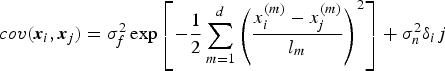 $$cov({\bi x}_i,{\bi x}_j) = \sigma _f^2 \exp \left[ - \displaystyle {1 \over 2} \sum\limits_{m = 1}^d \left( \displaystyle x_i^{(m)} - x_j^{(m)} \over l_m \right)^2 \right] + \sigma _n^2 \delta _ij$$
where the  $\sigma _f^2 $ is the signal variable. The signal variable tunes up the uncertainty of predictions in areas of training data density. The $x_i^{(m)} $ and $x_j^{(m)} $ are the m th component of the vector xi and xj, respectively. The length scales of the process, l = [l 1, l 2, ⋯, l d], reflect the relative smoothness of the process along the different input dimension. The $\sigma _n^2 $ regulates the global noise of the process. The δ ij is the Kronecker function, ${\delta _{ij}} = \left\{ \matrix{1\;\;\;\;\;\;\;i = j \hfill \cr 0\;\;\;\;\;\;i \ne j \hfill} \right.$. The parameters θ = {l, σ f, σn} are referred to as hyper-parameters of the GP. They can be determined by maximizing the log marginal likelihood of the given training set (Ranganathan et al., Reference Ranganathan, Yang and Ho2011; Rasmussen et al., Reference Rasmussen, Christopher and Williams2006).
 $$\eqalign{{\hat {\bi \theta}} & = \arg \max \log \left(\,p\left(y \vert{\bi X},{\bi \theta}\right)\right) \cr & = \arg \max \left\{ { - \displaystyle{1 \over 2}{y^{\rm T}}{{\left[ {k(X,X) + \sigma _n^2 {I_n}} \right]}^ - }^1 y - \displaystyle{1 \over 2}\log \left\vert {k(X,X) + \sigma _n^2 {I_n}} \right\vert - \displaystyle{n \over 2}\log 2\pi } \right\}}$$
 The partial derivative of the function  $\hat \theta $ is the objective function for hyper-parameters estimation.
 $$\eqalign{& \nabla J({{\bi \theta} _r}) = \displaystyle{\partial \over {\partial {{\bi \theta} _r}}}\log (\,p(y\left\vert {{\bi X},{{\bi \theta}} )} \right.) \cr & \quad \quad \quad = \displaystyle{1 \over 2}tr\left\{ {\left[ {({\bi k}{{({\bi X},{\bi X})}^{ - 1}}{\bi y}){{({\bi k}{{({\bi X},{\bi X})}^{ - 1}}{\bi y})}^{\rm T}} - {\bi k}{{({\bi X},{\bi X})}^{ - 1}}} \right]\displaystyle{{\partial {\bi k}({\bi X},{\bi X})} \over {\partial {{\bi \theta} _r}}}} \right\}} $$
The optimisation problem can be worked out by the algorithm of scaled conjugate gradient descent. A detailed description of that algorithm can be found, for instance, in Chen et al. (Reference Chen, Cheng, Wang and Han2014).
(1) Initialize θ1, and set a margin of error eps > 0 and the maximum number N of iterations to avoid infinite iterations.
(2) For N iterations and $\left\vert {\nabla J({{\bi \theta} _r})} \right\vert \ge eps$, compute the gradient of the log marginal likelihood ∇J(θr);
(3) conserve the result as the direction of the steepest ascent q r = ∇J(θr);
(4) determine the optimal step size, λr , using golden point search, and then update θr + 1 = θr + λrqr;
(5) calculate the value of the objective function in the case of θr + 1 = θr + λrqr
(8)$${{\bi \theta} _{r + 1}} = \arg \max \log (\,p(y\left\vert {{\bi X},{{\bi \theta} _{r + 1}} = {{\bi \theta} _r} + {{\bi \lambda} _r}{q_r})} \right.)$$(6) go back to step (1) until the number of iterations reaches N.


Theoretically the hyper-parameters θ1 can be randomly assigned. However, because the optimisation problem is non-convex, there is no guarantee of acquiring a global optimum. Therefore, in order to avoid local maxima, the hyper-parameters θ1 can be well initialized as follows.
 $$\sigma _f^2 = \displaystyle{\alpha \over n}\sum\limits_{i = 1}^n {y_i^2} $$
 $$\sigma _n^2 = \displaystyle{{1 - \alpha} \over n}\sum\limits_{i = 1}^n {y_i^2} $$
 $${l_m} = \sqrt {\displaystyle{1 \over {2{n^2}\log 2}}\sum\limits_{i = 1}^n {\sum\limits_{\,j = 1}^n {{{\left\Vert {{{\bi x}_i} - {{\bi x}_j}} \right\Vert}^2}}}} \,m = 1,\;2,\; \cdots, \;d$$
here α is an empirical value, α ∈ [0,1].
3. METHODOLOGY
3.1. Data pre-processing
Daily time-series of LOD used in this contribution are collected from the IERS EOP 05 C04 series. The LOD data consist of periodic effects such as influences of the solid Earth tides with periods from five days up to 18·6 years, diurnal and semi-diurnal variations due to the ocean tides. These tidal variations are first removed from the observed LOD measurements by using the zonal and ocean tide models recommended in the IERS Conventions 2010 (Petit and Luzum, Reference Petit and Luzum2010). Hereafter, the time-series thus obtained are denoted as LODR after correcting the above-mentioned tidal variations for the LOD data.
3.2. Reduction of time-series
The LODR data still consist of a linear part and some seasonal variations such as annual and semi-annual oscillations. In order to avoid the error coming from the extrapolation problem, a linear trend and seasonal variations are reduced from the LODR time-series. To this end the parameters of a linear term and seasonal variations are estimated by the LS method from the LODR data: bias (a 0) and drift (a 1) of the linear term, amplitudes (A a, Asa) and phases (Φa, Φsa) of the annual and semi-annual oscillations. Hence the LS model including a one order polynomial and two sinusoids can be written as
 $${\,f_{{\rm LODR}}}(t) = {a_0} + {a_1}t + {A_a}({\omega _a}t + {\Phi _a}) + {A_{sa}}({\omega _{sa}}t + {\Phi _{sa}})$$
where ω a = 2π / 365.24 and ω sa = 2π / 182.62.
The selected LS deterministic model is subsequently used for two purposes: (1) to obtain stochastic residuals (the differences between the LODR data and LS model) and (2) to predict the deterministic components of the signal (extrapolation).
In Figure 1, the observed LOD and its representation by the LS model plus tidal models are plotted from 1 January 1990 to 31 December 2009. Let us note that the model f LOD(t) = f LODR(t) + tidal term is denoted by the a priori model. The residual time-series are also shown in Figure 1. The amplitude of the residuals (bottom plot (e)) is small in comparison with that of the original time-series (top plot (a)). This indicates that the a priori model represents the original LOD time-series rather well. The differences between the a priori model and actual LOD time-series are used for training the GPR.

Figure 1. Plot (a) represents the observed LOD; (b) represents the effects of zonal Earth tides plus ocean tides; (c) represents the effects of a linear trend plus the seasonal variations including annual and semi-annual oscillations; (d) as sum of (b) and (c) constructs the a priori model of LOD; and (e) illustrates the LOD residuals calculated as the differences between (a) and (d).
3.3. Generation of training patterns
After the LOD time-series have been reduced, the training patterns are formed. As described in Section 2, the GPR requires an input before it is able to yield an output. A first possibility is to utilise the variable time t as the only input for feeding the GPR. The residual value at the time t could then be employed to form the output of the GPR. Indeed, practical experiments have demonstrated that this procedure can represent the training patterns rather well, but forecasts nonetheless fail. This happens because the input variable t in the case of forecast has to be extrapolated into the future. As the values of the input data in the case of forecast, i.e. the extrapolated time t, are not covered by the training set, the GPR generates poor predictions.
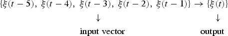
It turns out that for near-term predictions the values from the past few days are most essential. Consequently, a more sophisticated strategy is to utilise previous values as inputs of the GPR and future values as outputs. This strategy is based both on theoretical considerations concerning the time-varying characteristics of the stochastic residuals and on practical trials. Different training patterns have been implemented based on the strategy to find which perform best for the predictions of the residuals. We define the residual time-series as {ξ(i), i = 1, 2, ⋯, }. Then the values of the residual time-series of the last five days are selected as inputs and the day to be predicted is selected as an output. Such patterns are given as
 $$\eqalign{& \{ \xi (t - p - 4),\;\xi (t - p - 3),\;\xi (t - p - 2),\;\xi (t - p - 1),\;\xi (t - p)\} \to \{ \xi (t)\} \cr & \;\;\;\;\;\;\;\;\;\;\;\;\;\;\;\;\;\;\;\;\;\;\;\;\;\;\;\;\;\;\;\;\;\;\;\;\;\;\;\;\;\;\;\; \;\;\;\;\;\;\downarrow \;\;\;\;\;\;\;\;\;\;\;\;\;\;\;\;\;\;\;\;\;\;\;\;\;\;\;\;\;\;\;\;\;\;\;\;\;\;\;\;\;\;\;\;\;\;\;\;\;\;\;\;\;\;\; \downarrow \cr & \;\;\;\;\;\;\;\;\;\;\;\;\;\;\;\;\;\;\;\;\;\;\;\;\;\;\;\;\;\;\;\;\;\;\;\;\;\;\;\;\;\;{\rm input}\;{\rm vector \;\;\;\;\;\;\;\;\;\;\;\;\;\;\;\;\;\;\;\;\;\;\;\;\;\;\;\;\;\;\;\;\;\;\;\;\;\;\;\;\;\; output}} $$
for p = 1, 2, ⋯ , 360, where p is the number indicating the day in the future to be predicted. Each element of the input vector is close to each other, so the patterns are called the continuous patterns.
Similarly, the following patterns have also been generated.
 $$\eqalign{& \{ \xi (t - 5p),\;\xi (t - 4p),\;\xi (t - 3p),\;\xi (t - 2p),\;\xi (t - p)\} \to \{ \xi (t)\} \cr & \;\;\;\;\;\;\;\;\;\;\;\;\;\;\;\;\;\;\;\;\;\;\;\;\;\;\;\;\;\;\;\;\;\;\;\;\;\;\; \downarrow \;\;\;\;\;\;\;\;\;\;\;\;\;\;\;\;\;\;\;\;\;\;\;\;\;\;\;\;\;\;\;\;\;\;\;\;\;\;\;\;\;\;\;\;\;\;\;\;\; \downarrow \cr & \;\;\;\;\;\;\;\;\;\;\;\;\;\;\;\;\;\;\;\;\;\;\;\;\;\;\;\;\;\;\;\;{\rm input}\;{\rm vector \;\;\;\;\;\;\;\;\;\;\;\;\;\;\;\;\;\;\;\;\;\;\;\;\;\;\;\;\;\;\;\;\;\;\;\; output}} $$
for p = 1, 2, ⋯, 360. Since the interval between near elements of the input vector is p rather than 1, the patterns are denoted as the interval patterns, where the further the day to be forecasted is into the future, the further values in the past are required.
Considering the fact that the closer the observational data is to the day to be forecasted, the greater the impact on the prediction is, we form such patterns where the residuals of the last 1, 2, 3, 4 and 5 days are used to gain the residual value of the next day. Unlike other patterns, however, the patterns employ the predicted values as inputs for the next days to be predicted after the first day. Such patterns are composed as
 $$\eqalign{& \{ \xi (t - 5),\;\xi (t - 4),\;\xi (t - 3),\;\xi (t - 2),\;\xi (t - 1)\} \to \{ \xi (t)\} \cr & \;\;\;\;\;\;\;\;\;\;\;\;\;\;\;\;\;\;\;\;\;\;\;\;\;\;\;\;\;\;\;\;\;\;\;\; \downarrow \;\;\;\;\;\;\;\;\;\;\;\;\;\;\;\;\;\;\;\;\;\;\;\;\;\;\;\;\;\;\;\;\;\;\;\;\;\;\;\;\;\;\;\; \downarrow \cr & \;\;\;\;\;\;\;\;\;\;\;\;\;\;\;\;\;\;\;\;\;\;\;\;\;\;\;\;\;\;\;{\rm input}\;{\rm vector \;\;\;\;\;\;\;\;\;\;\;\;\;\;\;\;\;\;\;\;\;\;\;\;\;\;\;\;\; output}} $$
Because the patterns utilise the forecasted values as inputs in already existing models to compute the corresponding prediction values for the future days, such patterns are called the recursive patterns.
The above-formed pattern matrices are then switched along the entire time-series of the stochastic residuals, constructing a multitude of pattern pairs. On this basis the GPR is employed to infer the relationship between past input data and future data of the residual time-series.
4. PREDICTION RESULTS AND COMPARISON WITH OTHER METHODS
Daily time-series of the IERS EOP 05 C04 series, which span the time interval from 1 January 1990 to 31 December 2001, are used to train and validate the GPR model. The whole dataset is divided into two parts in such a way that the time-series from 1 January 1990 to 31 December 1999 are employed for training of the GPR model and the remaining part between 1 January 2000 and 31 December 2001 for validation of the GPR model.
The three pattern sets as described in Section 3.3 have been composed, and then used to train the GPR model, respectively. Then the well-trained GPR model is used to produce a predicted set of residuals for the future 1~10, 15, 20, 25, 30, 60, 90, …, and 360 days. Finally the resulting predicted value of the residuals for any particular day is added to the corresponding value of the a priori model to obtain the actual forecasted value of LOD. The comparison of different patterns is given in Figure 2 (in the meaning of the Root Mean Square (RMS) measure defined in Equation (13)). In Figure 2, it can be seen that the recursive patterns perform best out of three kinds of patterns until the 120th day. After the 120th day, the results from the continuous patterns are very close to those from the recursive patterns, but the latter is slighter better than the former. This difference may come from using predicted values that carry errors as inputs. Besides the high accuracy, the benefit of using the recursive patterns is mainly from the computational speed at the modelling stage. This is because we only set up a universal GPR model for the multi-step ahead predictions. In the following examples, the recursive patterns will be employed for training of the GPR model.
Figure 2. Comparison of RMS prediction errors of different patterns. Plot (a) and plot (b) represent RMS errors of short-term (up to 30 days) and medium-term (up to 360 days) predictions, respectively.
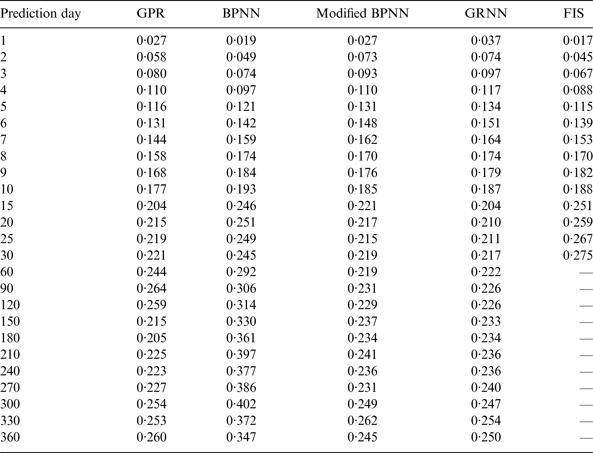
The RMS errors for different prediction intervals are listed in Table 1. The RMS error of the prediction day p is defined by
 $${\rm RM}{{\rm S}_p} = \sqrt {\displaystyle{1 \over l}\sum\limits_{i = 1}^l {{{(O_d^i - F_d^i )}^2}}} $$
with F the forecasted value of the developed method obtained for day p, O the actual value of the IERS C04 series, and l the number of predictions made for the particular prediction day. 365 predictions starting at different days have been made for each prediction day to compute the RMS error, i.e. l = 365.
Table 1. Comparison of GPR, FIS, BPNN, modified BPNN and GRNN RMS prediction errors (in units of ms).
The results of GPR predictions are compared with those obtained by other ML algorithms for medium-term predictions (Table 1), including Back-Propagation Neural Networks (BPNN) by Schuh et al. (Reference Schuh, Ulrich, Egger, Müller and Schwegmann2002), FIS by Akyilmaz and Kutterer (Reference Akyilmaz and Kutterer2004), modified BPNN and General Regression Neural Networks (GRNN) by Zhang et al. (Reference Zhang, Wang, Zhu and Zhang2012), which are found to be comparable with those of former approaches. Note that only short-term predictions were carried out by Akyilmaz and Kutterer (Reference Akyilmaz and Kutterer2004). In order to make the comparison illustrative, the RMS prediction errors obtained by different methods are shown in Figure 3. As can be seen in Figure 3 and Table 1, the proposed algorithm is able to provide predictions which are equal to or even better than those attained by other ML algorithms, except that the GPR predictions for the intervals of 1, 2, 3 and 4 days are slightly worse than those of BPNN and FIS, and for the intervals of 60, 90, 120 and 360 days worse than those of modified BPNN and GRNN. As for the prediction efficiency, the time taken by the developed strategy is noticeably less than that taken by other ML methods thanks to the used recursive patterns.
Figure 3. Comparison of RMS prediction errors of different ML algorithms. Plots (a) and (b) represent RMS errors of short-term (up to 30 days) and medium-term (up to 360 days) predictions, respectively.
It should be pointed out that the RMS errors shown here are obtained by testing the prediction methods over different prediction periods. This may have affected the results of the other authors, although we utilize the same equation for calculating the RMS error and the same LOD reference series (IERS C04 series). A final picture of the accuracy of different prediction methods could only be attained by a kind of contest where prediction spans and evaluation scheme are clearly specified in advance. Fortunately, the EOP Prediction Comparison Campaign (EOP PCC) lasting from October 2005 until February 2008 provides an opportunity to compare the performance of different prediction methods and techniques directly. Therefore, we have conducted a comparison with the results of the EOP PCC for the purpose of evaluating the prediction accuracy of the proposed algorithm. We have selected the LOD time-series which span the time interval between 30 September 1995 and 30 September 2005 as the data basis to forecast the LOD values for the future 1~500 days during the period from 1 October 2005 to 28 February 2008 (the same period as that of the EOP PCC). A comparison with other prediction methods and techniques which computed LOD predictions during the EOP PCC is shown in Figures 4 to 6, where the Mean-Absolute-Error (MAE) is selected as the statistical measure among the various statistical estimates. The MAE is calculated for the ith day in the future by the following.
 $${\rm MA}{{\rm E}_p} = \displaystyle{1 \over l}\sum\limits_{i = 1}^l {\left\vert {O_d^i - F_d^i} \right\vert} $$
The MAE given here is obtained by testing the prediction strategies over same prediction period and number. A list of participants who supported the LOD predictions can be found in Kalarus et al. (Reference Kalarus, Schuh, Kosek, Akyilmaz and Bizouard2010). What can be said with the information available from the comparison is that the accuracy of ultra short-term predictions by the GPR is inferior to the prediction accuracy of the number one (Gross et al. (Reference Gross, Eubanks, Steppe, Freedman, Dickey and Runge1998)) and the number two (Kalarus et al. (Reference Kalarus, Schuh, Kosek, Akyilmaz and Bizouard2010)). For short-term predictions an accuracy is obtained which is inferior to the best presently available prediction method developed by Gross et al. (Reference Gross, Eubanks, Steppe, Freedman, Dickey and Runge1998). In Figure 6, we can see that the GPR can provide predictions that are equal to or better than those of other methods until the 300th day. After the 300th day, the GPR predictions are getting slightly worse than those of the number one (Gross et al. (Reference Gross, Eubanks, Steppe, Freedman, Dickey and Runge1998)).
Figure 4. Comparison of MAE of ultra short-term (up to 10 days) predictions by the GPR and EOP PCC.
Figure 5. Comparison of MAE of short-term (up to 30 days) predictions by the GPR and EOP PCC.
Figure 6. Comparison of MAE of medium-term (up to 500 days) predictions by the GPR and EOP PCC.
5. CONCLUSIONS
GPR modelling is rather easy to use in comparison with ANN and FIS modelling. Inferring GPR models is a data-driven approach and thus the presented method can avoid human subjectivity and improve the credibility of predictions. The comparison with results of other methods clearly proves that GPR is a very promising tool to predict the variations in LOD. The recursive patterns perform best out of the three training pattern sets, although the patterns use predicted values as inputs for the next days to be forecasted. Besides the high accuracy, the recursive patterns require much less computation. Consequently, the application of the recursive patterns to LOD predictions can not only obtain the accurately predicted results, but can also substantially improve the prediction efficiency. LOD predictions will greatly benefit from the developed GPR-based technique using the recursive patterns since the availability of predicted EOP will be very fast, especially for short-term predictions. Despite the fact that we have set up GPR models with a single output, it is also possible to construct models with multiple outputs. In this case, the number of input variables used in GPR prediction models should also be increased. This may need much more attention while composing the optimal input and output patterns.
In spite of the good quality of predictions obtained so far, further improvements are possible as follows.
Additional a priori information entered into GPR models as an input variable may improve the results, mainly of the short-term predictions.
The predicted values of the atmospheric and oceanic excitation functions can be added into GPR models as pseudo-observational data, similar to what has been carried out in some other systems.
GPR is a kind of kernel-based ML algorithm and therefore the quality of derived models is strongly dependent on the kernel (covariance) function. As further work, a hybrid kernel function may be constructed for GPR so as to improve the prediction quality.
ACKNOWLEDGEMENTS
The authors are grateful to the IERS for providing LOD data, to M. Kalarus for providing the data of the EOP PCC, and to the anonymous reviewers for their remarks and advice on modifying the manuscript. This work is supported by the West Light Foundation of Chinese Academy of Sciences.