


1. Introduction
The mass balance of the Greenland ice sheet (GrIS) has been continuously negative for the past two decades with changes in the ice dynamics of tidewater glaciers (TWGs) contributing 40–60% to the total mass loss of the GrIS annually (Enderlin and others, Reference Enderlin2014; Mouginot and others, Reference Mouginot2019; Shepherd and others, Reference Shepherd2020). TWGs have undergone widespread multi-year retreat and thinning since the mid-1990s with TWG margins suggested to be particularly sensitive to changes in atmospheric and oceanic forcings (Rignot and others, Reference Rignot, Box, Burgess and Hanna2008; Nick and others, Reference Nick, Vieli, Howat and Joughin2009). However, assigning specific drivers of TWG retreat remain challenging (Cowton and others, Reference Cowton, Sole, Nienow, Slater and Christoffersen2018).
Previous studies have attributed the retreat of TWGs to warming climate and identified sea-ice concentration, runoff, sea surface temperatures (SSTs), deep water ocean temperatures (DWTs) and air temperatures (ATs) as potential factors that drive retreat (e.g. Bevan and others, Reference Bevan, Luckman and Murray2012; Carr and others, Reference Carr, Vieli and Stokes2013; Cowton and others, Reference Cowton, Sole, Nienow, Slater and Christoffersen2018; Wood and others, Reference Wood2018). However, the non-linearity of TWG behaviour, which is also dependent on hydrology, topography and ice dynamics (e.g. Meier and Post, Reference Meier and Post1987), alongside the scarcity of oceanic and atmospheric observations, has prevented the confident determination of the relative influence of different climate drivers (Straneo and others, Reference Straneo2013; Morlighem and others, Reference Morlighem2017). Analysing records of the past behaviour of Greenland's TWGs in detail on an ice-sheet-wide scale therefore provides the opportunity to gain further insights into the response of their marine terminating margins to climate forcings, helping to better assess Greenland's potential future contribution to global sea level change.
Achieving these insights requires a comprehensive ice-sheet-wide, multi-decadal dataset of terminus observations (cf. King and others, Reference King2020) that also capture the full variability of terminus shape (i.e. through using variations on the ‘box method’ of terminus change measurement (Moon and Joughin, Reference Moon and Joughin2008; Lea and others, Reference Lea2014)) and are as near as possible temporally homogeneous (i.e. where observations are taken at the same time of year). Recent advances in tools that enable rapid review of available imagery and direct mapping of TWG margins from freely available satellite data means that this is now feasible (Lea, Reference Lea2018).
Previous studies have investigated the behaviour of TWGs in Greenland, however, they were limited to either specific areas of the GrIS (e.g. Khan and others, Reference Khan2014; Hill and others, Reference Hill, Carr, Stokes and Gudmundsson2018), specific temporal ranges (e.g. Moon and Joughin, Reference Moon and Joughin2008; Murray and others, Reference Murray2015; Bunce and others, Reference Bunce, Carr, Nienow, Ross and K2018) or to only the fastest flowing TWGs (e.g. Bevan and others, Reference Bevan, Luckman and Murray2012; Andersen and others, Reference Andersen2019; Jochemsen, Reference Jochemsen2019). Groups of different TWGs in different sectors have generally been shown to be retreating since the mid-1990s (Bevan and others, Reference Bevan, Luckman and Murray2012; Hill and others, Reference Hill, Carr, Stokes and Gudmundsson2018) and that bedrock topography and fjord geometry coupled with external climate forcings are strongly influencing their behaviour (Bevan and others, Reference Bevan, Luckman and Murray2012; Carr and others, Reference Carr, Vieli and Stokes2013; Khan and others, Reference Khan2014; Catania and others, Reference Catania2018, Reference Catania, Stearns, Moon, Enderlin and Jackson2020). However, the varying spatio-temporal scales of previous studies have made it difficult in many cases to quantitatively determine multi-decadal sector-wide and ice-sheet-wide patterns of TWG behaviour and to investigate regional factors that drive TWG retreat.
Here, we present a record of annual terminus positions for 206 TWGs around the GrIS from 1984 to 2017. The extensive spatio-temporal scale of the observations presented here (Fig. 1) allows investigation of TWG behaviour and their drivers on a regional scale, in contrast to undertaking site specific assessments of individual TWG terminus change (e.g. Howat and others, Reference Howat, Joughin, Tulaczyk and Gogineni2005; Lea and others, Reference Lea2014; Brough and others, Reference Brough, Carr, Ross and Lea2019). The resulting regional patterns of TWG behaviour are placed into context and quantitatively compared with AT, SST and runoff anomalies as well as solid ice flux to investigate the individual and sector-wide responses of TWGs in Greenland to a warming climate (Cowton and others, Reference Cowton, Sole, Nienow, Slater and Christoffersen2018; King and others, Reference King2020).

Fig. 1. Location of TWGs for which margin data are available in the dataset (points coloured by region) on top of Greenland Mapping Project (GIMP) DEM (Howat and others, Reference Howat, Negrete and Smith2014). The regions (black lines) were determined based on the surface ice divides of the GrIS, which were identified using the same GIMP DEM (Rignot and Mouginot, Reference Rignot and Mouginot2012; Howat and others, Reference Howat, Negrete and Smith2014). The inset map shows a panchromatically sharpened Landsat 8 image from 3 August 2019 overlaid with digitised margins for Helheim Glacier as an example for the available margin data.
2. Data and methods
2.1 Dataset creation and normalisation
We digitised the margins of 224 TWGs directly discharging from the GrIS (i.e. excluding any peripheral ice caps), including 153 named TWGs (Bjørk and others, Reference Bjørk, Kruse and Michaelsen2015) and an additional 71 unnamed TWGs (named UN_XX in the dataset). The terminus dataset was created using the Google Earth Engine Digitisation Tool (GEEDiT) and was quantified using the Margin Change Quantification Tool (MaQIT) (Lea, Reference Lea2018). An annual record of complete ice margins (n = 3801) was manually digitised by a single operator from NASA Landsat 4-8 satellite imagery, complemented by European Space Agency Sentinel 2 imagery, spanning an observation period from 1984 to 2017. The image resolution of 30 m allowed the digitisation of TWGs with a margin width down to 500 m. Data gaps associated with the scan line corrector failure on Landsat 7 were linearly interpolated if the gaps did not include the lateral TWG–bedrock border. In instances where shadows of fjord walls or clouds obscured small parts of the TWG margin, the margin was interpolated through the concealed area if <10% of the total length of the TWG margin were obscured and the concealed area did not include the lateral TWG–bedrock border. If more than 10% of the TWG or the lateral TWG–bedrock border was obscured, the image was not used for margin digitisation.
The error for manual digitisation using GEEDiT was quantified for Landsat 4 imagery by repeated digitisation (n = 10) of three different TWG margins and calculating the root mean squared error (e.g. Moon and others, Reference Moon, Joughin and Smith2015; Bunce and others, Reference Bunce, Carr, Nienow, Ross and K2018) and for Landsat 8 by a previous study (Brough and others, Reference Brough, Carr, Ross and Lea2019). The mean error lies between ±5.6 m for Landsat 4 and ±3.6 m for Landsat 8, which is less than the pixel resolution of the imagery used.
To ensure homogeneity of the dataset between annual observations and to aid subsequent analyses, margins were only digitised where imagery was available in September towards the end of the melt season, when TWGs are typically at their annual minimum extent. All available satellite images for the month of September in each year were evaluated to determine the most suitable image (ideally cloud-free and unobstructed by shadows) for manual digitisation so that the quality of the resulting dataset is consistent. The analyses in this study were conducted on 206 of the 224 digitised TWG margins, as the northern sector was excluded from detailed analysis due to a lack of observations (results are reported for reference in Figure S1).
The margin changes over time were quantified using the curvilinear box method within MaQiT. This is an extension of the box method (Moon and Joughin, Reference Moon and Joughin2008) which has the benefit of being able to continuously track fjord orientation as the TWG advances/retreats (Lea and others, Reference Lea2014). The method provides a notable advantage over the centreline method of tracking TWG change as it is able to account for the full terminus geometry rather than a highly localised part of the TWG margin that may produce results that are not representative of overall margin position (Lea, Reference Lea2018). Absolute values of margin change were normalised between 0 (most retreated) and 1 (most advanced) using min-max feature scaling (Eqn (1)). The normalisation factors out the absolute magnitude of individual terminus change, which is dependent on glacier size and terminus width (ranging from several metres to kilometres). This allows individual glacier and ice-sheet sector behaviour to be compared on a common scale:

To identify trends in the records of TWG change segmented regression was applied, using global optimisation to fit line segments to the data points (Fig. 3, panels (i)). This determines the most suitable break point locations by solving a least squares fit for a set number of times (n = 1000) (Jekel and Venter, Reference Jekel and Venter2019). For comparison, we also applied robust locally weighted regression (LOWESS) using an f-value (smoothing span) of 0.25 and three iterations to make the weighted regression more robust.
2.2 Climate data
2.2.1 Sea surface temperatures
SSTs were taken from the monthly HadISST v1 dataset (1° latitude–longitude resolution) and, for the regional analysis, averaged for all sectors, which were determined by the ice divides (Rayner and others, Reference Rayner2003; Howat and others, Reference Howat, Negrete and Smith2014). The dataset was limited to only comprise data within a fixed distance of 150 km from the coast (Fig. 2a). The buffer was based on the simplified coastline of Greenland with the resulting data being averaged annually from October to September starting the year preceding the observation. In order to derive individual SST values for each investigated TWG, a k-nearest neighbour analysis (KD-Tree) was conducted to identify the four gridpoints of the HadISST v1 dataset with the smallest Euclidian distance (Minkowski distance p = 2) to the respective glacier (Figs S8–S229). The KD-Tree method uses decision trees and k-nearest neighbour algorithms to determine the nearest neighbours, which reduces computational time compared to alternative methods. The corresponding SST anomalies were derived with respect to the 1961–90 baseline.
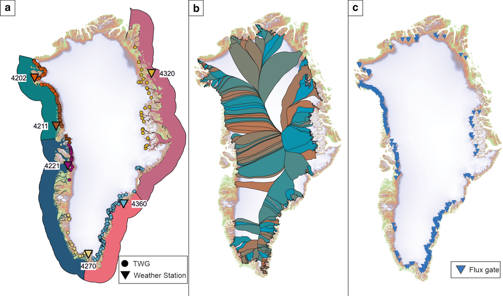
Fig. 2. (a) Overview TWG locations, weather stations and SST buffers used in the analyses. AT data were selected from six DMI weather stations (marked with the corresponding station code; Cappelen, Reference Cappelen2014) and matched to individual TWGs using a nearest neighbour distance matrix. The TWGs (circles) are colour-coded corresponding to the weather station (triangle) used in the analyses. The 150 km regional buffers used to average SSTs are taken from the HadISST v1 dataset (Rayner and others, Reference Rayner2003), and are shown colour-coded by region. In the northern sector of the GrIS, high sea ice concentrations impact the availability of usable data thus it is excluded here. (b) Catchment areas used to determine annual runoff anomalies (Mouginot and Rignot, Reference Mouginot and Rignot2019). (c) Locations of flux gates used in the determination of annual mean solid ice flux (Mankoff and others, Reference Mankoff2019). Background images show surface elevation based on GIMP DEM (Howat and others, Reference Howat, Negrete and Smith2014).
2.2.2 Deepwater ocean temperatures
DWTs from the World Ocean Atlas 2018 were only available as decadal averages thus not used in subsequent quantitative analysis, although provide useful context to observations. Available DWT anomalies in proximity to the TWG margin are provided in Supplementary data for reference (Locarnini and others, Reference Locarnini2018). DWT anomalies were derived using the 1981–2010 baseline for shallow (0–50 m with measurements every 10 m) and deep-water (0–1000 m with measurements every 100 m) profiles (Figs S8–S229). A KD-Tree analysis was conducted on the DWT gridpoints to determine the four points with the smallest Euclidian distance to the respective TWG. The resulting gridpoints were further limited to locations within 50 km from the coastline to ensure that the derived anomalies represent conditions at the glacier margin as close as possible.
2.2.3 Air temperatures
AT data were selected from six weather stations (Fig. 2a) from the Danish Meteorological Institute (DMI) (Cappelen, Reference Cappelen2014) and averaged for seasonal intervals (September–October–November = SON, December–January–February = DJF, March–April–May = MAM, June–July–August = JJA). As terminus positions were digitised in September, ATs were taken starting in the September of the preceding year to include a complete seasonal interval (e.g. SON).
Inland fjord locations of the weather stations were favoured over coastal locations to better represent conditions at the TWG margins and minimise the influence of sea fog/maritime climate on the data (cf. Taurisano and others, Reference Taurisano, Bøggild and Karlsen2004).
The 1961–90 average was chosen to calculate AT and SST anomalies as it provides a climate baseline during a period that comprises relative mass-balance neutrality (Bjørk and others, Reference Bjørk2012; Mouginot and others, Reference Mouginot2019). The TWG specific AT anomalies were derived by determining the closest weather stations to the individual location of the TWG within each ice-sheet sector (Fig. 2a). All seasonal AT anomalies for each sector can be found in Figure S2.
2.2.4 Runoff
Glacier specific runoff was determined using daily data from the regional climate model (MAR) v3.9 with a 10 km grid and individual catchment areas (Fig. 2b) (Fettweis and others, Reference Fettweis2012; Mouginot and Rignot, Reference Mouginot and Rignot2019). The catchments are based on a combination of ice flow and surface topography data to represent water flow direction (Mouginot and others, Reference Mouginot2019). The original runoff data were converted from millimetre w.e. to gigatonnes. Runoff anomalies were derived using the 1961–90 baseline (Fig. S2).
2.2.5 Solid ice flux
Ice flux data used in this study (Mankoff, Reference Mankoff2019) are derived using flux gates, which are transects upstream of the terminus, enabling the determination of solid ice flux as ice velocities and volumes at these gates are measured over time. The dataset used here is based on algorithmically picked flux gates rather than manually picked gates and includes only data for ice flowing faster than 100 m a−1 (Mankoff, Reference Mankoff2019; Mankoff and others, Reference Mankoff2019). The spatial resolution of the data from which the fluxes are derived is 200 m × 200 m per pixel, with flux gate widths ranging from 3 to 392 pixels. Temporal resolution is dependent on data availability and ranges from monthly (1986–2015) up to every 6 days (2015–17) (Mankoff and others, Reference Mankoff2019).
Flux gate locations were matched manually with each individual glacier location in order to determine the absolute annual solid ice flux for each glacier. Some glaciers did not have a flux gate in place, so that no discharge data were available (Fig. 2c). For glaciers with more than one flux gate, the ice flux measured by all gates was summed. If one flux gate was available for two or more glaciers, the data were assigned to each glacier, as no definitive split could be determined. For each TWG, the annual deviation from the 1986–2017 mean in percentage was determined using Eqn (2), with D dev being the relative ice flux deviation from the mean in percent, D being the annual ice flux (September to August), and D mean being 1986–2017 mean annual ice flux (Fig. 3, panels (ii)):


Fig. 3. (i) Annually averaged normalised terminus positions, (ii) normalised ice flux anomalies expressed as percentage deviation from the mean, (iii) black line shows the difference between number of TWGs with increase in flux and number of TWGs with decrease in flux, bars show number of TWGs with advancing/retreating terminus, (iv) SST anomalies and (v) JJA AT anomalies for (a) NW sector, (b) NE sector, (c) SW sector and (d) SE sector. Regional trends are shown using segmented regression (black) and local regression (LOWESS; light green), std dev. (±1σ) is shown in light grey.
For each sector, the resulting data were subsequently averaged for all TWGs for each year (Fig. 3 and Fig. S3). To investigate the relationship between ice flux and sustained retreat, we identified the TWGs within each sector with the largest ice fluxes. Ice flux in the northwestern (NW) sector is generally increasing over the investigated time frame, however no single TWG dominates (Mouginot and others, Reference Mouginot2019). Therefore, we identified the TWGs with the largest ice flux in the NW sector as those having a >1.5 Gt a−1 change in ice flux, calculated as the difference between the 2017 value and the 1986–2000 mean. In the southwestern (SW) and southeastern (SE) sector, previous studies identified Sermeq Kujalleq (Jakobshavn Isbræ), Helheim Glacier and Kangerlussuaq Glacier, respectively, as TWGs experiencing the greatest changes in flux in their respective region (Howat and others, Reference Howat, Joughin, Tulaczyk and Gogineni2005; Rignot and Kanagaratnam, Reference Rignot and Kanagaratnam2006; Stearns and Hamilton, Reference Stearns and Hamilton2007).
2.3 Statistical analyses
A hierarchy of statistical tests was used to determine the influence of climate drivers on regional and individual TWG behaviour. The analyses comprised of (i) linear correlation for each sector; (ii) Engle–Granger cointegration tests for each sector and individual TWGs to test for spurious correlation and (iii) Johansen test to investigate the climate forcings for cointegration.
Pearson correlation coefficients for climate forcings and regional normalised terminus change are shown in Figures S4–S6. Investigation for spurious regression between climate variables and margin change was undertaken with two Engle–Granger tests, performed on (i) climate and terminus data for each individual TWG and (ii) averaged margin change and representative climate data for each sector as a whole. These determined whether terminus response and each of the climate drivers were cointegrated on a glacier-by-glacier basis, and regional basis respectively (Table 1) (Granger and Newbold, Reference Granger and Newbold1974; Engle and Granger, Reference Engle and Granger1987; Cowton and others, Reference Cowton, Sole, Nienow, Slater and Christoffersen2018). The test assesses the statistical relationship between two non-stationary time series requiring a single dependent variable (i.e. terminus change) to be chosen (Table 1).
Table 1. Correlation coefficients (Pearson's R), and p values obtained from the linear regression for each region (n = number of TWGs in sector) and climate variable. Regional Engle–Granger h-value indicating cointegration (0 = no cointegration, 1 = cointegration) and corresponding p values. Percentage of cointegrated TWGs determined by Engle–Granger test for individual TWGs and climate forcings, out of the total number of TWGs in the sector. Statistically significant (p < 0.05) linear regression p values and Engle–Granger h-values are shown in bold

Correlation coefficients (Pearson's R), and p values obtained from the linear regression for each region (n = number of TWGs in sector) and climate variable. Regional Engle–Granger h-value indicating cointegration (0 = no cointegration, 1 = cointegration) and corresponding p values. Percentage of cointegrated TWGs determined by Engle–Granger test for individual TWGs and climate forcings, out of the total number of TWGs in the sector. Statistically significant (p < 0.05) linear regression p values and Engle–Granger h-values are shown in bold.
Cross-correlation of climate forcing anomalies was first analysed using heatmaps with the derived p values indicating strong inter-variable dependencies (Fig. S7). The majority of p values passed a significance threshold of 0.05, thus disqualifying the possibility of using multiple regressions to determine if correlations between different climate forcings exist. Consequently a Johansen test for cointegration was conducted to determine whether a relationship exists between the individual climate forcings (Johansen, Reference Johansen1991).
The Johansen test is an extension of the Engle–Granger test, as it enables the investigation of multiple time series with each other and does not require the selection of a dependent variable (Table S1). It conducts a cointegration test for each variable against the remaining variables with the results showing the respective test statistic (named test in Table S1) and critical values at varying confidence levels (namely 10, 5 and 1%). The variables, which correspond to the matrix rank, are cointegrated if the test statistic of the input variable is larger than the critical value (Pfaff and others, Reference Pfaff, Zivot, Stigler and Pfaff2016). In this study, the Johansen test was conducted for seven variables (namely, SST anomalies, runoff anomalies, solid ice flux, SON anomalies, DJF anomalies, MAM anomalies and JJA anomalies) and the results show that cointegration exists up to the 6th matrix rank (i.e. for all climate variables).
The Engle–Granger test allows to determine if a single variable (i.e. one of the climate forcings) is cointegrated with a dependent variable (i.e. normalised TWG margin change). If two variables show cointegration, it further strengthens the significance of the Pearson correlation coefficient, whereas no cointegration suggests spurious regression and the correlation coefficient should be regarded with caution. The Johansen test in contrast, analyses all variables with each other for cointegration. Used together, they enable the conclusion that while a single climate driver might show a high Pearson correlation coefficient and Engle–Granger cointegration, it is ultimately also dependent on all other climate forcings.
3. Results
3.1 Linear terminus response of sectors
Segmented and LOWESS regression revealed linear retreat trends of normalised terminus change across all sectors of the GrIS (Fig. 3). It was determined that the trends across each sector can be captured using segmented regression with one inflection point (IP). While a greater number of IPs were explored, and for some sectors they display a closer fit to the data on timescales of 2–3 years, one IP is able to capture overall behaviour for every sector over 5–10-year timescales. One IP is also found to be broadly consistent with results of LOWESS regression. In the SW, NW and SE sectors of the GrIS we found regional trends of stability/minor advance until the mid-1990s, followed by sustained retreat until the end of the observation period in 2017 (Figs 3a, c, d). Overall retreat is near ubiquitous, with 92.2% (190 of 206) of TWGs retreating.
Unlike other sectors, the northeast (NE) shows a trend of sustained linear retreat from the beginning of the observational period (1984), followed by accelerated retreat starting in 2004/05 (Fig. 3b).
3.2 Potential drivers of terminus change
Potential mechanisms to explain this GrIS-wide linear retreat were explored both qualitatively and through the hierarchy of statistical approaches described (see Section 2.3). The onset of glacier retreat along with higher, sustained positive regional SST and JJA AT anomalies is apparent for all ice-sheet sectors (Fig. 3). In the NE sector (Fig. 3b), continuously high SST anomalies accompany normalised TWG retreat from the start of the observation period, whereas the acceleration of normalised TWG retreat (2002–03) is preceded by 3 years of increasingly positive SST and JJA AT anomalies, that have previously been linked to a reduction in sea-ice concentration (Khan and others, Reference Khan2014). In the SW, NW and SE sectors, the onset of sector-wide retreat is accompanied by increasingly positive SST, runoff and AT anomalies (Figs 3a, c, d), making qualitative separation of the relative importance of oceanic and atmospheric forcing in these regions impossible.
Significant negative correlations (p < 0.05) between normalised regional TWG terminus change and climate forcings occur across all sectors (Fig. 4 and Figs S4–S6), although significant cross-correlation of climate variables casts doubt on assigning causal links to specific climate variables (Fig. S7). Investigation for spurious regression between climate variables and normalised margin change revealed that on a regional scale, SST anomalies in the NW sector and JJA AT anomalies in the SE sector are cointegrated with sector-wide terminus change. Other climate variables were found to exhibit no cointegration with normalised terminus change, meaning that all remaining significant correlation coefficients identified are likely to be spurious (Table 1).

Fig. 4. Correlation between normalised terminus change and mean annual SST anomalies (°C), annual runoff anomalies (Gt a−1) and JJA AT anomalies (°C) for the NW and SE sectors of the GrIS. Pearson's correlation coefficient, R 2 and corresponding p values shown for each correlation. Correlations for all sectors and climate variables can be found in Figures S4–S6.
Glacier-by-glacier analysis shows that 28.2% (n = 58) of all analysed TWGs exhibit some manner of cointegration to one or more climate variables (Fig. 5 and Table 1), although the Johansen test results identify the climate variables to be cointegrated with each other (Table S1).

Fig. 5. Cointegration of TWG margin change to climate. (a) TWGs in each sector that show cointegration to one or more climate forcings cointegrated TWGs (light green points), grouped by region and geographically sorted (north to south) on top of surface elevation base map (Howat and others, Reference Howat, Negrete and Smith2014). The specific cointegration for each individual TWG is indicated by a green square. (b) Percentages of TWGs cointegrated to individual climate forcing in each sector.
The majority of individual TWGs that are cointegrated with climate in the NW and SE exhibit terminus responses that are related to SST and JJA AT anomalies respectively (Fig. 5). These results are consistent with results of the regional scale cointegrations (Table 1). However, significant numbers of TWGs in all sectors show cointegration between terminus change and other climate drivers.
3.3 Terminus change versus glacier flux
While ice fluxes of the GrIS have been increasing in absolute terms (Enderlin and others, Reference Enderlin2014; King and others, Reference King2018; Mankoff and others, Reference Mankoff2019), normalised ice flux anomalies averaged by sector (where each glacier is equally weighted) are shown to be consistent over the investigated time period (Figs 3, 6). This stability is despite 92.2% of TWGs retreating over the investigated time period. This is further supported by the relative, sector-wide consistency of the number of TWGs that show an increase/decrease of flux (Fig. 3, panels (iii)).
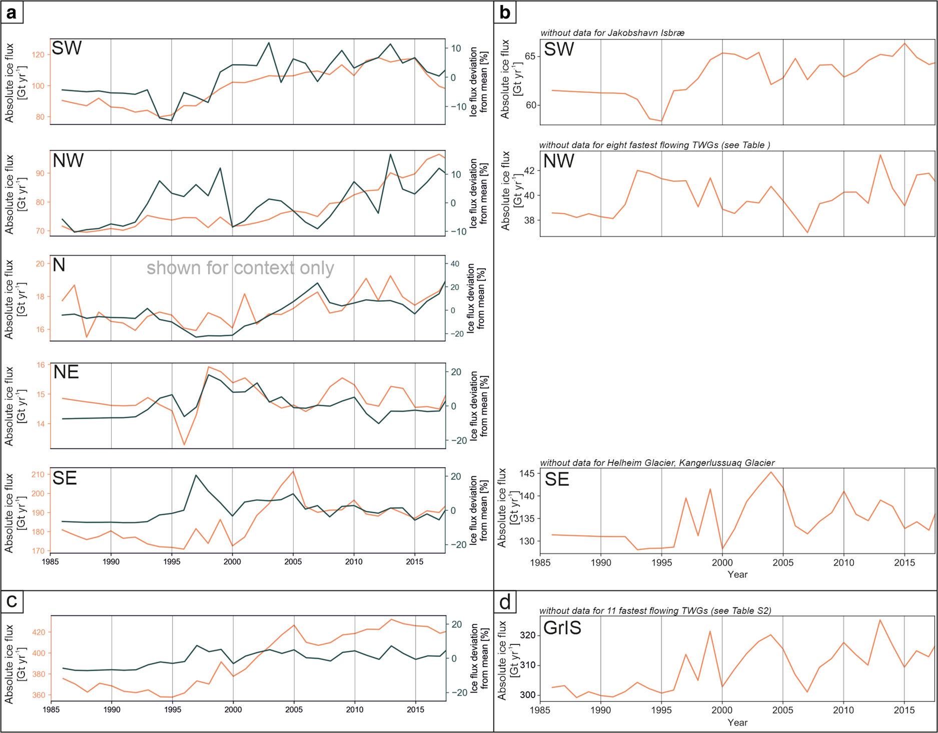
Fig. 6. Ice fluxes of each sector with and without fastest flowing TWGs. (a) Sum of absolute ice flux for all sectors in Gt a−1 (orange) and normalised ice flux anomalies expressed as percentage deviation from the mean (dark green; as shown in Fig. 3, panel (ii)) and (b) sum of absolute ice flux in Gt a−1 for the SW sector without data for Jakobshavn Isbræ, for the NW sector without eight fastest flowing TWGs (Table 2) and for the SE sector without data for Helheim Glacier and Kangerlussuaq Glacier. Note the different y-axis limits and their ranges. (c) Sum of absolute ice flux for all sectors of the GrIS (including north sector) and (d) Sum of absolute ice flux for all sectors of the GrIS without 11 glaciers with largest ice flux (see Table 2).
Ice fluxes from individual TWGs have high spatio-temporal variability due to the dependency on glacier geometry, bedrock topography and seasonal dynamics (Howat and others, Reference Howat, Joughin and Scambos2007; Catania and others, Reference Catania2018; King and others, Reference King2018; Slater and others, Reference Slater2019). However, the largest TWGs disproportionately impact regional ice flux trends by skewing it towards an increase, with the combined fluxes of 11 glaciers (total of 3985.29 Gt for 1986 to 2017) able to account for 75.7% of the observed increase in flux between 1986 and 2017 (Fig. 6b and Table 2). Once these large glaciers are removed from the record, the total absolute ice flux of all other TWGs combined remains relatively stable over the investigated time period. Consequently, the total sector-wide fluxes of the overwhelming majority of TWGs remains consistent during sustained terminus retreat (Fig. 6).
Table 2. Eleven TWGs that have the largest contribution on the overall flux increase in their respective region (see section ‘Methods’), with geographic location (Lat, Lon), total retreat, average ice flux during a period of stability, ice flux for 2017 and flux difference

Eleven TWGs that have the largest contribution on the overall flux increase in their respective region (see section ‘Methods’), with geographic location (Lat, Lon), total retreat, average ice flux during a period of stability, ice flux for 2017 and flux difference.
4. Discussion
The large spatio-temporal scale of the dataset of TWG margins created for this study allowed the identification of linear regional TWG retreat patterns in all sectors of the GrIS analysed (Fig. 3). Previous research identified individual TWG response to climate as non-linear with the onset of retreat in most regions starting in the mid-1990s to early 2000s (Bevan and others, Reference Bevan, Luckman and Murray2012; Rignot and Mouginot, Reference Rignot and Mouginot2012; Hill and others, Reference Hill, Carr, Stokes and Gudmundsson2018). Although our results are consistent with these findings for individual TWGs, when multiple TWG responses are normalised and averaged by sector, retreat is found to be linear over decadal time scales despite the complexities induced by localised bed topography and ice dynamics (Fig. 3). These results are also consistent with the wider relationships of TWG behaviour across the GrIS and climate suggested by Slater and others (Reference Slater2019). The linear behaviour of normalised terminus change found in this study corroborates their hypothesis that TWG margin behaviour may be homogeneous when analysed over greater spatio-temporal timescales.
Sustained linear TWG retreat since 1984 was also identified in the NE sector, contrasting with previous observations from the North East Greenland Ice Stream (NEGIS) basin, where retreat for the period 1984–2004 was not identified (Khan and others, Reference Khan2014; Velicogna and others, Reference Velicogna, Sutterley and van den Broeke2014). Given that each TWG has equal weighting in our analysis and includes TWG margins for the entire sector, it should be noted that our results do not discount the stability of NEGIS during this time, but rather demonstrate that TWG margins have on average been retreating in the NE sector for 34 years. To explain this behaviour, it is likely that either the 1961–90 climate baseline conditions were not conducive to multi-annual to decadal terminus stability in this sector, or that prior to 2000 the NE sector as a whole experienced a longer term lagged response to earlier climate forcing.
The onset of regional linear TWG retreat in all sectors is accompanied by an increase of all climate forcings analysed (ATs, SSTs and runoff), however determining the influence of individual climate variables on TWG behaviour is not straightforward (Cowton and others, Reference Cowton, Sole, Nienow, Slater and Christoffersen2018; Slater and others, Reference Slater2019). Using a hierarchy of statistical tests, Pearson correlation coefficients indicated relationships between SSTs and terminus change in the NW and SW sectors, and between ATs and terminus change in the NE and SE sectors. While this might suggest that these climate forcings might be the key drivers of TWG retreat across these sectors, Engle–Granger cointegration tests performed on the regional data showed that only the results for the NW and SE sector can be considered not to be spurious (Table 1).
Identification that 28.2% (n = 58) of all investigated TWGs exhibit cointegration with one or more climate forcings (Fig. 5) highlights the complexity of ice–ocean–atmosphere interactions on a local scale, showing that even neighbouring TWGs might respond differently to climate. Therefore, at an individual TWG scale and over short-term time scales of less than 5 years, upstream ice dynamics, bedrock topography and fjord geometry will modulate its sensitivity to climate (Bevan and others, Reference Bevan, Luckman and Murray2012; Carr and others, Reference Carr, Vieli and Stokes2013; Khan and others, Reference Khan2014; Catania and others, Reference Catania2018; Cowton and others, Reference Cowton, Sole, Nienow, Slater and Christoffersen2018). However, when considering TWG retreat over decadal to multi-decadal time scales for each sector of the ice sheet, the effect of topography and upstream ice dynamics is diminished leading to an overall linear retreat pattern.
Cowton and others (Reference Cowton, Sole, Nienow, Slater and Christoffersen2018) previously identified a similar linear response to oceanic and atmospheric warming for 10 TWGs along Greenland's east coast between 1993 and 2012. Their results also revealed that when viewed at timescales of a few years or more (>5 years) the influence of topographic pinning points diminished and TWG margin retreat did not deviate far from a linear response to climate warming. Although the approach in this study differs, our results show that this finding is not likely to be limited to the subset of glaciers analysed by Cowton and others (Reference Cowton, Sole, Nienow, Slater and Christoffersen2018), but does hold more broadly across the SW, NW, NE and NW sectors of the GrIS.
The results from the Johansen cointegration test show that all climate forcings are cointegrated (Table S1), which further indicates that TWG behaviour is likely influenced by a complex combination of climate drivers rather than a single climate forcing (Straneo and others, Reference Straneo2013; Slater and others, Reference Slater2020). However, the cointegration of TWGs in the NW sector to SST anomalies and in the SE sector to JJA AT anomalies revealed by the Engle–Granger test suggests that sufficient variability in the climate data exists to identify that these two climate forcings are likely to play a more dominant role than others in the respective sectors.
In contrast to the sustained regional retreat of TWGs, our results show that total sector-wide solid ice flux remained relatively stable for the majority of glaciers over the investigated time period (Fig. 3 and Fig. S3) (Mankoff and others, Reference Mankoff2019). The overall absolute increase in flux in the NW, SW and SE sectors, observed between sector-wide periods of stability (1986–2000 for NW, SE; 1986–95 for SW) and 2017, can be attributed to the 11 TWGs with the largest changes in ice flux (Fig. 6 and Table 2). This is highlighted in Figures 6c, d, where these TWGs are shown to account for 75.7% of increase in flux in the NW, SW and SE sectors. In a previous study, King and others (Reference King2020) determined a solid ice flux increase of ~60 Gt a−1 between the 1980s and 2018 for the entirety of the GrIS, with results presented here indicating that more than half of this total flux increase of the GrIS can be explained by only 11 glaciers, which show a solid ice discharge increase of 37.5 Gt (Table 2). This suggests that the majority of TWGs in these sectors did not experience a long-lived increase in flux despite undergoing margin retreat, or increases were offset by other TWGs experiencing decreases in their flux (Enderlin and others, Reference Enderlin2014; King and others, Reference King2018).
Consequently, at a regional scale, sustained TWG retreat does not necessarily equate to an increase in flux for each sector, with the exception of the influence of a small number of individual glaciers. However, it should be noted that while the grounding line position of the majority of Greenlandic TWGs roughly coincides with the terminus position (Kehrl and others, Reference Kehrl, Joughin, Shean, Floricioiu and Krieger2017), there are multiple TWGs often in northern regions of the ice sheet that either possess floating ice tongues that are either perennial or seasonal. Although this study has not sought to capture seasonal terminus dynamics, the loss of seasonal or perennial ice tongues may lead to future sustained increases in velocities and solid ice flux for more TWGs then identified in Table 2 (e.g. Joughin and others, Reference Joughin2008; Hill and others, Reference Hill, Carr, Stokes and Gudmundsson2018; Bevan and others, Reference Bevan, Luckman, Benn, Cowton and Todd2019; Brough and others, Reference Brough, Carr, Ross and Lea2019; Mouginot and others, Reference Mouginot2019).
The heterogeneity of TWGs around Greenland and uncertainties regarding fjord bathymetry, bedrock topography and atmosphere–ice–ocean interactions currently pose a major challenge for ice-sheet scale models (Aschwanden and others, Reference Aschwanden2019; Slater and others, Reference Slater2019). However, the confirmation of consistent sector-wide fluxes alongside ice-sheet-wide linear retreat patterns offers significant potential for the simplification of modelling efforts for the overwhelming majority of outlets (e.g. Slater and others, Reference Slater2019). To capture multi-decadal changes in ice-sheet flux it may only be necessary to undertake detailed modelling of only the largest outlet glaciers, or those that have the potential for a sustained increase in ice flux (e.g. Felikson and others, Reference Felikson, Catania, Bartholomaus, Morlighem and Noël2020; Mouginot and others, Reference Mouginot2019).
5. Conclusion
This study presents a comprehensive dataset of annual Greenland-wide TWG margins for 1984–2017 utilising new methods for their rapid mapping. By placing margin change for each TWG on a relative scale we are able to directly compare every TWG irrespective of how much or how little it has changed. Results from these analyses show the existence of regionally linear and multi-decadal TWG retreat for SE, SW and NW sectors that initiated in the mid-1990s. Previously unidentified sustained retreat in the NE sector for the entire observational period is also shown, including an acceleration in retreat from approximately 2004. These results indicate that TWG margins across the entire ice sheet are in disequilibrium with the current climate, with the linear trends identified showing that the TWGs of each sector as a whole are responding to this imbalance.
Cointegration analysis allowed the rejection of spurious correlations between terminus changes and climate drivers, while also successfully highlighting the sensitivity of TWG margins to SST and JJA AT anomalies in the NW and SE sectors respectively. These findings are supported by cointegration analysis between individual TWG records and climate within each region, identifying potentially contrasting drivers of TWG change even between neighbouring glaciers. Pinpointing drivers behind individual TWG behaviour therefore still remains challenging.
The identification of widespread retreat alongside regionally consistent ice fluxes on multi-decadal timescales potentially negates the requirement to directly model every individual outlet of the GrIS, and only those that demonstrate (or have the potential for) a sustained increase in ice flux need to be considered. This offers the opportunity for current ice-sheet models to be run with significantly lower computational costs and model complexity with respect to TWG margin dynamics. Such modelling approaches would benefit those seeking to explore wider ranges of climate forcing scenarios impacting the GrIS within both ice dynamic and atmospheric/ocean coupled ice-sheet models, and those seeking to improve estimates of Greenland's contribution to sea level change.
Supplementary material
The supplementary material for this article can be found at https://doi.org/10.1017/jog.2021.13.
Data
The terminus margin data can be found at 10.5281/zenodo.4327594.
Acknowledgements
DF acknowledges support for this study through the EPSRC and ESRC Centre for Doctoral Training on Quantification and Management of Risk and Uncertainty in Complex Systems Environments Grant No. EP/L015927/1. JML and SB are supported by a UKRI Future Leaders Fellowship (Grant No. MR/S017232/1). We thank Martin Olsen at Asiaq Greenland Survey for providing comments on the manuscript. We thank the Scientific Editor Frank Pattyn and two reviewers for their helpful and insightful comments.
Author contributions
DF and JML conceived the study. DF produced the dataset, conducted all data analysis, figure production and led the manuscript writing. JML and SB provided conceptual and technical advice. JML, SB, DWFM and JA contributed to the writing of the manuscript.
Conflict of interest
The authors declare no competing financial interests.


 Open access