


1. Introduction
In the wake of a currency devaluation and debt crisis in 2002, the government of Argentina reinstituted export taxes on a wide range of products, including soybeans, with the goal of increasing fiscal revenues and limiting the devaluation’s impact on inflation (Regúnaga and Rodriguez, Reference Regúnaga and Rodriguez2015). Initial rates were set at 13.5% for soybeans and 5% for soybean oil. In the years that followed, the government continued to increase export tax rates. By 2007, export taxes on soybeans and soybean oil were at their highest levels, 35% and 32%, respectively. There was even an attempt to further increase soybean export taxes in 2008, which was never implemented because of nationwide protests by farmers (Pirovano, Reference Pirovano2009; Regúnaga and Rodriguez, Reference Regúnaga and Rodriguez2015; Sandoval and Joseph, Reference Sandoval and Joseph2015).
Argentina has a long history of taxing agricultural exports. Taxes on soybean exports have been particularly high relative to other agricultural products given their importance to the overall economy and foreign exchange earnings. Despite this history, a newly elected government in 2015 has been committed to economic reforms, implementing policies to decrease or eliminate exports taxes on principal agricultural commodities such as dairy, beef, corn, wheat, and soybeans (Sullivan and Nelson, Reference Sullivan and Nelson2017). In 2016, there was an immediate export tax reduction of 5% on soybean products, but because of fiscal concerns it was later determined that further reductions would be delayed until 2018. The plan was to reduce soybean export taxes by 0.5% per month from January 2018 until December 2019 (Sandoval, Reference Sandoval2016; Sullivan and Nelson, Reference Sullivan and Nelson2017). However, because of a worsening economy, the Argentine government imposed another suspension of export tax reductions and announced in September 2018 that soybeans and soybean products will be subject to a fixed and variable export tax rate until December 2020. Currently, the fixed rate for all soybean products is 18%, and the variable rate is 4 Argentine pesos per U.S. dollar in export value, which varies in percentage terms based on the exchange rate (Sandoval, Reference Sandoval2018).
Argentina’s attempt at export tax reform raises questions about the performance and competitiveness of its soybean sector. Although rate reductions could improve farmer profitability, the global effects of this policy are not obvious. Argentina is the world’s third leading soybean exporter, but it exports are a fraction of the exports from the United States and Brazil (e.g., about 20% of Brazil’s exports in 2016). Given Argentina’s position in the global soybean trade, it is conceivable that a reduction or elimination of export taxes could improve its global competitiveness, displacing soybean exports from countries like the United States and Brazil. However, because Argentina exports significantly less than the United States and Brazil, it is also conceivable that its export tax reform could have little effect on competing countries and global markets. An important objective of this study is to determine which outcome (significant impact as opposed to little effect on global markets) is the most likely.
China’s soybean market provides the ideal case for examining how Argentina’s export tax reform will affect major exporting countries. China is the largest foreign soybean market and is particularly important to global export disappearance (Chen, Marchant, and Muhammad, Reference Chen, Marchant and Muhammad2012). For instance, China imported more than 80 million metric tons (MT) of soybeans in 2016, accounting for almost two-thirds of global soybean trade; its imports from Argentina were 8 million MT, accounting for more than 80% of Argentina’s export disappearance. China is also important to the United States and Brazil, accounting for 60%–80% of soybean exports from these countries.Footnote 1
In this study, we examine the factors that determine China’s demand for imported soybean products. Of particular importance is the price competition between Argentina, Brazil, and the United States and how the elimination of export taxes in Argentina could affect Chinese imports. A primary objective of this study is to estimate China’s demand for imported soybeans and soybean oil differentiated by exporting source.Footnote 2 We employ an estimation procedure that allows for deriving unconditional import demand elasticities, which can account for both trade diversion and creation when examining the impact of price-changing policies. These estimates are then used to project the impact of Argentina’s export tax reform on China’s import demand by exporting source.
Although Argentina exports significantly less than the United States and Brazil, a price shock in Argentina could still affect soybean prices globally. Taking this into account, we assess the long-run price relationship among soybean products in Argentina, Brazil, and the United States, as well as in China, using a vector autoregression (VAR) model. Given the import demand and VAR estimates, we conduct import demand projections assuming the following: (1) prices in Argentina are the only prices affected by its export tax reform; (2) prices in Brazil, the United States, and China experience the largest possible response to Argentina’s export tax reform based on the estimated relationships from the VAR procedure; and (3) prices in all countries reached their long-run equilibrium as specified by the estimated relationships from the VAR procedure. Monte Carlo simulations are used to derive confidence intervals for all projections based on the covariance matrix of the estimated import demand coefficients.
Overall, most studies of export tax reform in Argentina have been relatively broad in scope (Bouët, Estrades, and Laborde, Reference Bouët, Estrades and Laborde2014; Deese and Reeder, Reference Deese and Reeder2007; Meilke, Wensley, and Cluff, Reference Meilke, Wensley and Cluff2001). Cicowiez, Díaz-Bonilla, and Díaz-Bonilla (Reference Cicowiez, Díaz-Bonilla and Díaz-Bonilla2010) examined the long-run effect of export tax elimination on economic growth and poverty mitigation in Argentina, and Toulan (Reference Toulan2002) assessed the impact of export tax, import tariff, and export subsidy eliminations on world demand for Argentine exports. More specific to Chinese soybean demand, Taheripour and Tyner (Reference Taheripour and Tyner2018) and Muhammad and Smith (Reference Muhammad and Smith2018) examine the impact of the U.S.-China trade war on Chinese soybean imports. Studies of how export taxes in Argentina affect soybean import demand in China appear to be absent from the literature.
The remainder of this article is structured as follows. We close this section with an overview of China’s soybean product imports. In Section 2, we present the model and simulation procedure. We then give an overview of the data, estimation, report estimates, and simulation results (Section 3). The final section contains a brief summary and conclusion Section 4).
1.1. China’s soybean product imports
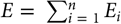
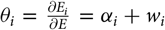
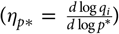
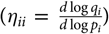
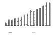
China’s soybean and soybean oil imports are reported in Figure 1, China’s soybean imports by source are reported in Figure 2, and China’s import value and value shares are reported in Table 1. Since 2002, China’s imports have significantly increased from $3 billion (all dollar amounts are in U.S. dollars) to about $35 billion (11 million MT to about 84 million MT in volume), an increase of more than 1,000%. Overall, soybeans (HS 1201 soybeans, whether or not broken) account for the majority of China’s soybean product imports. Since 2007, soybean oil (HS 1507 soybean oil and its fractions, whether or not refined, but not chemically modified) as a share of total imports has been declining, accounting for less than 2% in 2016. The share of China’s soybean product imports from the United States has remained relative stable since 2002 (30%–40%), whereas the share of imports from Brazil has increased to about 45% in recent years. From 2007 to 2012, the United States was China’s leading foreign supplier (in volume). Since that time, Brazil has reemerged as China’s leading soybean supplier. In 2016, China imported 38 million MT of soybeans from Brazil and 34 million MT from the United States, but only 8 million MT from Argentina.

Figure 1. China’s soybean and soybean oil imports: 2002–2016. Source: World Trade Atlas, Global Trade Information Services Inc.

Figure 2. China’s soybean imports by source: 2002–2016. Source: World Trade Atlas, Global Trade Information Services Inc.
Table 1. Soybean imports in China and exporter and product shares: 2002–2016

a ROW is the rest of the world.
Source: World Trade Atlas, Global Trade Information Services Inc.
Particularly interesting is the decline in imports and market share for Argentina starting in 2009–2010. The currency devaluation in 2002 resulted in relative stable exports to China. During the period 2002–2008, Argentina remained a leading exporter of soybean oil, reflecting the country’s large and growing crushing capacity and export tax structure that favored soybean oil and biodiesel rather than soybeans. Beginning in 2009, however, a financial crisis constrained Argentina’s soybean product exports. This decline was also attributable, in part, to government policies that created disincentives for agricultural production and exports and, more recently, higher returns to competing crops such as corn and wheat (Regúnaga and Rodriguez, Reference Regúnaga and Rodriguez2015). Since recovering from a low in 2009 (4 million MT) to a high in 2010 (11.2 million MT), China’s soybean imports from Argentina have been consistently less than 10 million MT.
2. Methods
2.1. Import demand model
We use an Armington (Reference Armington1969) framework (source differentiation) to model China’s soybean import demand. In this context, soybeans (or soybean oil) from the ith exporting country are treated as an individual good that is part of the product group imported soybeans and an imperfect substitute for soybeans from other exporting countries.Footnote 3 Within and across exporting countries, there is also imperfect substitutability between products (soybeans vs. soybean oil).
Following Seale, Marchant, and Basso (Reference Seale, Marchant and Basso2003) and Muhammad (Reference Muhammad2013), a differenced version of the Almost Ideal Demand System (AIDS) is employed for estimation (Deaton and Muellbauer, Reference Deaton and Muellbauer1980). Like other differential demand systems, the differenced AIDS is linear in coefficients and is therefore easy to estimate. Additionally, first differencing variables for empirical analysis can alleviate problems of nonstationarity (Matsuda, Reference Matsuda2005). The AIDS functional form is also suitable when there are periodic disruptions in trade because log quantities are not needed for estimation (Muhammad, Reference Muhammad2013). We discuss the issue of modeling trade disruptions in more detail later in the section.
We denote the price and quantity of China’s soybeans imports from the ith exporting country as p i and q i, respectively, and China’s total expenditure on all soybean imports as $E = \mathop \sum \nolimits_{i = 1}^n {E_i}$
, where E i = p iq i is the value of imports from exporting country i and n is the total number of exporting countries/products. We also denote the import expenditure share for exporting country i as w i = E i/E. Given these terms, the first-differenced AIDS is specified as follows:
$E = \mathop \sum \nolimits_{i = 1}^n {E_i}$
, where E i = p iq i is the value of imports from exporting country i and n is the total number of exporting countries/products. We also denote the import expenditure share for exporting country i as w i = E i/E. Given these terms, the first-differenced AIDS is specified as follows:
 $$\Delta {w_{it}} = {\alpha _i}\Delta \ln\frac{{{E_t}}}{{{P_t}}} + \mathop\sum \limits_{j=1}^n {\beta _{ij}}\Delta \ln{p_{jt}} + \mathop\sum \limits_{k=1}^4 {\gamma _{ik}}{d_k} + {\mu _{it}}.$$
Δw it = w it - w it - 1 is the differenced import share; Δln E t = ln E t - ln E t−1 and Δln p jt = ln p jt - ln p jt−1 are the total expenditure and jth import price in log differences; and Δln P t is the Divisia price index: ${\Delta \ln {P_t} = \mathop \sum \nolimits_{i=1}^n {\mathop{\overline{w}}\nolimits_{it}}\Delta \ln {p_{it}},\, \rm where \,{\mathop{\overline{w}}\nolimits_{it}}} = 0.5\left( {{w_{it}} + {w_{it - 1}}} \right)$
is the average import share between periods t and t − 1. Unlike the Stone price index, which is typically used when estimating the AIDS functional form in levels, estimates using the Divisia price index are invariant to unit of measure (Seale, Marchant, and Basso, Reference Seale, Marchant and Basso2003). d k is a quarterly binary variable, added to account for seasonality, and μ is a random disturbance term. α, β, and γ are fixed parameters to be estimated. According to theory, the following parameter restrictions should hold true: Σiα i = Σiβ ij = Σiγ ik = 0 (adding up); Σjβ ij = 0 (homogeneity); and β ij = β ji (symmetry).
${\Delta \ln {P_t} = \mathop \sum \nolimits_{i=1}^n {\mathop{\overline{w}}\nolimits_{it}}\Delta \ln {p_{it}},\, \rm where \,{\mathop{\overline{w}}\nolimits_{it}}} = 0.5\left( {{w_{it}} + {w_{it - 1}}} \right)$
is the average import share between periods t and t − 1. Unlike the Stone price index, which is typically used when estimating the AIDS functional form in levels, estimates using the Divisia price index are invariant to unit of measure (Seale, Marchant, and Basso, Reference Seale, Marchant and Basso2003). d k is a quarterly binary variable, added to account for seasonality, and μ is a random disturbance term. α, β, and γ are fixed parameters to be estimated. According to theory, the following parameter restrictions should hold true: Σiα i = Σiβ ij = Σiγ ik = 0 (adding up); Σjβ ij = 0 (homogeneity); and β ij = β ji (symmetry).
From equation (1), we can derive the marginal import share, ${\theta _i} = \frac{{\partial {E_i}}}{{\partial E}} = {\alpha _i} + {w_i}$
, which is the additional expenditure on the ith import given a unit increase in aggregate import expenditures; conditional expenditure elasticity,
${\theta _i} = \frac{{\partial {E_i}}}{{\partial E}} = {\alpha _i} + {w_i}$
, which is the additional expenditure on the ith import given a unit increase in aggregate import expenditures; conditional expenditure elasticity, $\eta _i^* = \frac{{d\log {E_i}}}{{d\log E}} = 1 + {\alpha _i}/{w_i}$
, which is the additional expenditure on the ith import in percentage terms given a 1% change in aggregate import expenditures; and Slutsky price elasticity (Chalfant, Reference Chalfant1987):
$\eta _i^* = \frac{{d\log {E_i}}}{{d\log E}} = 1 + {\alpha _i}/{w_i}$
, which is the additional expenditure on the ith import in percentage terms given a 1% change in aggregate import expenditures; and Slutsky price elasticity (Chalfant, Reference Chalfant1987):
 $$\eta _{ij}^{\rm{*}} = \frac{{d\log q_i^{\rm{*}}}}{{d\log {p_j}}} = - {\delta _{ij}} + \frac{{{\beta _{ij}}}}{{{w_i}}} + {w_j}.$$
δ ij is the Kronecker delta; δ ij = 1 when i = j and 0 otherwise. Note that the Slutsky price elasticity $( {\eta _{ij}^*} )$
measures the impact of a 1% price change in exporting country j on China’s imports from exporting country i, holding real aggregate expenditures constant (substitution effect only).
$( {\eta _{ij}^*} )$
measures the impact of a 1% price change in exporting country j on China’s imports from exporting country i, holding real aggregate expenditures constant (substitution effect only).
2.2. Modeling trade disruptions
A feature of China’s demand for imported soybeans is periodic disruptions in trade, particularly when importing from Argentina. Disruptions in trade are problematic for import demand analysis because prices do not exist when trade is zero. Following Muhammad (Reference Muhammad2013) and Kuchler and Arnade (Reference Kuchler and Arnade2016), we use a choke-price procedure to account for periods of zero trade and unobserved prices.Footnote 4
To derive choke prices, we start with a general own-price elasticity equation $\left( {\eta _{ii}^* = \frac{{d\log {q_i}}}{{d\log {p_i}}}} \right)$
to get the following relationship:
$\left( {\eta _{ii}^* = \frac{{d\log {q_i}}}{{d\log {p_i}}}} \right)$
to get the following relationship: $\frac{{{{\mathop q\limits^{\prime } }_i} - {{\mathop q\limits^ - }_i}}}{{{{\mathop q\limits^ - }_i}}} = \eta _{ii}^*\frac{{{{\mathop p\limits^{\prime } }_i} - {{\mathop p\limits^ - }_i}}}{{{{\mathop p\limits^ - }_i}}}$
, which relates percentage deviations from the average quantity to percentage deviations from the average price. Setting
$\frac{{{{\mathop q\limits^{\prime } }_i} - {{\mathop q\limits^ - }_i}}}{{{{\mathop q\limits^ - }_i}}} = \eta _{ii}^*\frac{{{{\mathop p\limits^{\prime } }_i} - {{\mathop p\limits^ - }_i}}}{{{{\mathop p\limits^ - }_i}}}$
, which relates percentage deviations from the average quantity to percentage deviations from the average price. Setting ${\mathop{q_i}\limits^{\prime }} = 0$
and then solving for
${\mathop{q_i}\limits^{\prime }} = 0$
and then solving for ${\mathop{p_i}\limits^{\prime }}$
yields the following:
${\mathop{p_i}\limits^{\prime }}$
yields the following:
 $${\mathop{p_i}\limits^{\prime} = \left( {\frac{{\eta _{ii}^{\rm{*}} - 1}}{{\eta _{ii}^{\rm{*}}}}} \right){\mathop p\limits^ - }_i}.$$
Note that equation (3) is the price at which the quantity decreases from its mean value to zero. Equations (1), (2), and (3) are estimated via a two-step procedure repeated until convergence. See Muhammad (Reference Muhammad2013) for a more detailed discussion of this estimation procedure.
2.3. Estimating total import demand
It is important to account for both trade creation and diversion when analyzing the impact of prices on trade. Export tax reform in Argentina could affect prices in Argentina, resulting in Chinese importers substituting across exporting sources (trade diversion), but price changes could also affect China’s aggregate import expenditures (trade creation).
To account for the impact of price changes on aggregate import expenditures, we estimate China’s total import demand for soybeans. In this context, total import demand is based on the notion that imported soybean products are (or can be) “resold” to firms within China for further processing. Following Theil (Reference Theil1980), the relationship between total import demand and prices is specified by the following Divisia quantity index relationship:
 $$\Delta \ln\frac{{{E_t}}}{{{P_t}}} \cong {\rm{\Delta }}{Q_t} = {\rm{\Theta }}\left[ {\Delta \ln p_t^{\rm{*}} - \Delta \ln P_t^{\rm{'}}} \right].$$
The variable p * denotes a representative domestic/output price, which reflects the price that imported soybeans receive if resold in China, and $\Delta \ln P_t{^\prime} $
is the Frisch import price index, which is an average measure of import prices. The Frisch import price index is defined as follows:
$\Delta \ln P_t{^\prime} $
is the Frisch import price index, which is an average measure of import prices. The Frisch import price index is defined as follows:
 $$\Delta \ln{{P}}_{{t}}^{\rm{'}} = \mathop\sum \limits_{{j}} {{\rm{\theta }}_{{j}}}\Delta \ln{{{p}}_{{{jt}}}}.$$ ${\theta _j} = \frac{{\partial {E_j}}}{{\partial E}}$
is the marginal import share for exporting country j, and Δln p jt = ln p jt − ln p jt − 1 is the jth import price in log differences.
${\theta _j} = \frac{{\partial {E_j}}}{{\partial E}}$
is the marginal import share for exporting country j, and Δln p jt = ln p jt − ln p jt − 1 is the jth import price in log differences.
Θ is the Frisch price effect, which is assumed positive because an increase in China’s domestic/output price makes importing soybeans more profitable, holding other factors constant. A positive Frisch price effect also indicates an inverse relationship (−Θ) between the import price index $\left(\Delta\ln P_t^{'}\right)$
and China’s aggregate import expenditures
$\left(\Delta\ln P_t^{'}\right)$
and China’s aggregate import expenditures $\left( {\Delta \ln \frac{{{E_t}}}{{{P_t}}}} \right)$
.
$\left( {\Delta \ln \frac{{{E_t}}}{{{P_t}}}} \right)$
.
We use equations (2), (4), and (5) and the conditional expenditure elasticity $(\eta _i^*)$
to derive the unconditional price elasticity:
$(\eta _i^*)$
to derive the unconditional price elasticity:
 $${\eta _{ij}} = \frac{{d\log {q_i}}}{{d\log {p_j}}} = - \eta _i^*{\theta _j}{\rm{\Theta }} + \eta _{ij}^*.$$
The first term is the total import effect (trade creation), which is the effect of prices on imports through changes in total import expenditures. The second term is the direct effect of prices on imports as measured by equation (2), which accounts for the substitution across exporting countries because of changes in relative prices (trade diversion).
2.4. Import demand projections
We use elasticity-based forecasting equations to make import demand projections (Kastens and Brester, Reference Kastens and Brester1996):
 $${q_{i\left( 1 \right)}} = \biggl( {{\eta _{p*}}\frac{{p_{\left( 1 \right)}^* - p_{\left( 0 \right)}^*}}{{p_{\left( 0 \right)}^*}} + \mathop\sum \limits_j{\eta _{ij}}\frac{{{p_{j\left( 1 \right)}} - {p_{j\left( 0 \right)}}}}{{{p_{j\left( 0 \right)}}}}} \biggr){q_{i\left( 0 \right)}} + {q_{i\left( 0 \right)}}.$$
According to equation (7), the quantity imported from country i in the projection period is a function of the quantity imported during the base period, and the percentage changes in the domestic price and source-specific import prices from the base period to the projection period.Footnote 5
A number of studies have compared model- and elasticity-based forecasts using demand systems (Gustavsen and Rickertsen, Reference Gustavsen and Rickertsen2003; Kastens and Brester, Reference Kastens and Brester1996; Muhammad, Reference Muhammad2007). All have concluded that demand forecasts using elasticities are superior to model-based forecasts.
For the import demand projections, we assume the full elimination of export taxes and that taxes are fully passed through to import prices. Although this may not be the case, our projections can be considered as upper bound responses. First, we consider a scenario where prices in Argentina are the only prices affected by its export tax reform (short run). Then we consider outcomes where prices in the United States, Brazil, and China respond to price changes in Argentina. To derive the price response across countries, we estimate impulse response functions (IRFs) using a VAR model:
 $${{{\bf{p}}_t} = {{{{\bf A}}}_0} + {{\bf{{A}}}_1}{{\bf{p}}_{t - 1}} + {{\bf{{A}}}_2}{{\bf{p}}_{t - 2}} + \ldots+ {{\bf{{A}}}_k}{{\bf{p}}_{t - k}} + {\bf \epsilon}_t}.$$
p is the vector of prices (in levels) for Argentina, Brazil, the United States, and China. A0 is a vector of constants, Ai is a square coefficient matrix, k is the lag order, and ϵ is a vector of random disturbances. The advantage of using levels is that the estimates remain consistent regardless of prices being integrated or not. Furthermore, standard inference on impulse responses in levels will remain asymptotically valid, and the inference is asymptotically the same even in the presence of cointegrated prices (Lütkepohl and Reimers, Reference Lütkepohl and Reimers1992; Sims, Stock, and Watson, Reference Sims, Stock and Watson1990).
3. Estimation and results
3.1. Data and import demand estimation
We used quarterly import data (2002:1–2016:4) from the World Trade Atlas (https://www.gtis.com/gta/) to estimate soybean import demand in China by product and exporting source. We considered two products for the analysis: soybeans (HS 1201 soybeans, whether or not broken) and soybean oil (HS 1507 soybean oil and its fractions, whether or not refined, but not chemically modified). The soybean exporting countries included the United States, Brazil, and Argentina, and the soybean oil exporting countries included Brazil, Argentina, and the rest of world (ROW). China’s domestic soybean price, provided by the China National Grain and Oils Information Center, was used in estimating total import demand.
We estimated the import demand system represented by equation (1) using the generalized Gauss-Newton method in TSP (version 5.0), which is a maximum likelihood procedure for equation systems (Hall and Cummins, Reference Hall and Cummins2009). We tested and corrected for autoregressive disturbances using a procedure for singular equation systems (Beach and MacKinnon, Reference Beach and MacKinnon1979). The homogeneity and symmetry restrictions were imposed and tested using likelihood ratio tests. Test results indicated that homogeneity and symmetry could not be rejected at the 0.05 significance level.Footnote 6
We assumed the following empirical form for equation (4) to estimate China’s total import demand:
 $$\Delta \ln\frac{{{E_t}}}{{{P_t}}} = {{\rm{\Theta }}_0} + {{\rm{\Theta }}_1}\Delta \ln p_t^{\rm{*}} + {{\rm{\Theta }}_2}\Delta \ln P_t^{\rm{'}} + \mathop\sum \limits_{k = 1}^3 {{\rm{\Theta }}_{ik}}{d_k} + {\mu _t}.$$
Our results show that the estimated domestic/output price effect ${\widehat {\rm{\Theta }}_1} = 0.69(0.33)$
and import price effect
${\widehat {\rm{\Theta }}_1} = 0.69(0.33)$
and import price effect ${\widehat {\rm{\Theta }}_2} = - 0.46\left( {0.23} \right)$
are consistent with theory and significant at the 0.05 level.Footnote 7 Estimates indicate that given a 1% increase in the domestic/output price, China’s aggregate expenditures on soybean product imports increase by 0.69%, and given a 1% increase in the import price level, China’s aggregate expenditures on soybean product imports decrease by 0.46%.
${\widehat {\rm{\Theta }}_2} = - 0.46\left( {0.23} \right)$
are consistent with theory and significant at the 0.05 level.Footnote 7 Estimates indicate that given a 1% increase in the domestic/output price, China’s aggregate expenditures on soybean product imports increase by 0.69%, and given a 1% increase in the import price level, China’s aggregate expenditures on soybean product imports decrease by 0.46%.
3.2. Import demand elasticities
The conditional expenditure elasticity $(\eta _i^*)$
, domestic/output price elasticity (η p*), and unconditional own-price elasticities (η ii) are reported in Table 2.
$(\eta _i^*)$
, domestic/output price elasticity (η p*), and unconditional own-price elasticities (η ii) are reported in Table 2.
Table 2. Demand elasticities for soybean imports in China

a ROW is the rest of the world.
Notes: Asterisks (***, **, and *) respectively denote the 0.01, 0.05, and 0.10 significance level. Asymptotic standard errors are in parentheses.
Recall that the conditional expenditure elasticity $(\eta _i^* = \frac{{d\log {E_i}}}{{d\log E}})$
measures the percentage responsiveness of a given import to a 1% change in China’s aggregate import expenditures. Expenditure elasticity estimates are positive and significant for U.S. soybeans (0.58), Brazilian soybeans (1.27), Argentine soybeans (1.96), and Brazilian soybean oil (0.78). The expenditure elasticities for Argentina and Brazil are larger than the United States reflecting the fact that overall import growth in China has been because of relatively larger increases in imports from Latin America. The negative estimate for ROW soybean oil (–2.84) is likely the result of being a residual category rather than being an inferior product in the Chinese market.
$(\eta _i^* = \frac{{d\log {E_i}}}{{d\log E}})$
measures the percentage responsiveness of a given import to a 1% change in China’s aggregate import expenditures. Expenditure elasticity estimates are positive and significant for U.S. soybeans (0.58), Brazilian soybeans (1.27), Argentine soybeans (1.96), and Brazilian soybean oil (0.78). The expenditure elasticities for Argentina and Brazil are larger than the United States reflecting the fact that overall import growth in China has been because of relatively larger increases in imports from Latin America. The negative estimate for ROW soybean oil (–2.84) is likely the result of being a residual category rather than being an inferior product in the Chinese market.
The domestic/output price elasticity $({\eta_{p*}} = \frac{{d\log {q_i}}}{{d\log {p^*}}})$
measures how a 1% increase in China’s domestic price affects imports from each country. The results indicate that Argentine soybeans are the most responsive to an increase in China’s domestic price (1.36). The responsiveness of Brazilian soybeans (0.88) and U.S. soybeans (0.40) to the domestic price is significantly smaller. The responsiveness of soybean oil imports to the domestic price is insignificant for all exporting sources.
$({\eta_{p*}} = \frac{{d\log {q_i}}}{{d\log {p^*}}})$
measures how a 1% increase in China’s domestic price affects imports from each country. The results indicate that Argentine soybeans are the most responsive to an increase in China’s domestic price (1.36). The responsiveness of Brazilian soybeans (0.88) and U.S. soybeans (0.40) to the domestic price is significantly smaller. The responsiveness of soybean oil imports to the domestic price is insignificant for all exporting sources.
The unconditional own-price elasticities $({\eta_{ii}} = \frac{{d\log {q_i}}}{{d\log {p_i}}})$
indicate that Chinese demand for imported soybeans is relatively more elastic than soybean oil. The unconditional own-price elasticities for soybeans range from −1.75 for Brazil to −1.21 for Argentina. Comparably smaller in magnitude are the unconditional own-price elasticities for soybean oil: Brazil (−0.81) and Argentina (−0.85). ROW soybean oil is the most sensitive to own-price changes (−1.92), likely because of China’s relatively small imports from ROW.
$({\eta_{ii}} = \frac{{d\log {q_i}}}{{d\log {p_i}}})$
indicate that Chinese demand for imported soybeans is relatively more elastic than soybean oil. The unconditional own-price elasticities for soybeans range from −1.75 for Brazil to −1.21 for Argentina. Comparably smaller in magnitude are the unconditional own-price elasticities for soybean oil: Brazil (−0.81) and Argentina (−0.85). ROW soybean oil is the most sensitive to own-price changes (−1.92), likely because of China’s relatively small imports from ROW.
The unconditional cross-price elasticities $({\eta_{ij}} = \frac{{d\log {q_i}}}{{d\log {p_j}}})$
are reported in Table 3. Results indicate that the relationship between countries and products are mostly insignificant. Exceptions include substitute relationships between soybeans from the United States and Brazil, soybean oil from Brazil and Argentina, and soybean oil from Brazil and ROW.
$({\eta_{ij}} = \frac{{d\log {q_i}}}{{d\log {p_j}}})$
are reported in Table 3. Results indicate that the relationship between countries and products are mostly insignificant. Exceptions include substitute relationships between soybeans from the United States and Brazil, soybean oil from Brazil and Argentina, and soybean oil from Brazil and ROW.
Table 3. Unconditional cross-price elasticities (η ij) for soybean imports in China

a ROW is the rest of the world.
Notes: Asterisks (*** and **) respectively denote the 0.01 and 0.05 significance level. Asymptotic standard errors (SE) are in parentheses.
3.3. VAR estimation and impulse response functions
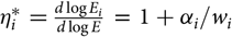
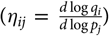
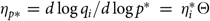
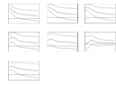
IRFs, based on generalized standard-deviation impulses as described by Pesaran and Shin (Reference Pesaran and Shin1998), are used to assess the impact of price shocks in Argentina on prices in other countries. IRFs for soybean price shocks in Argentina are shown in Figure 3, and IRFs for soybean oil price shocks in Argentina are shown in Figure 4.

Figure 3. Generalized impulse responses to innovations in soybean prices in Argentina. Notes: Vertical axes measure generalized standard-deviation impulses as described by Pesaran and Shin (Reference Pesaran and Shin1998). The 95% confidence bans (dotted lines) are based on Monte Carlo standard errors.

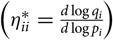
Figure 4. Generalized impulse responses to innovations in soybean oil prices in Argentina. Notes: Vertical axes measure generalized standard-deviation impulses as described by Pesaran and Shin (Reference Pesaran and Shin1998). The 95% confidence bans (dotted lines) are based on Monte Carlo standard errors.
Note that after a soybean price shock in Argentina (Figure 3), soybean prices in the United States, Brazil, and China and soybean oil prices in Brazil and Argentina respond similarly. However, the confidence bans for the responsiveness of soybean oil prices in Argentina are comparably large. After the fifth quarter, the confidence bans for all prices include the zero axis, which is an indication that the responses to soybean price shocks in Argentina are not long lasting.
Results are even less compelling for soybean oil price shocks in Argentina (Figure 4) where soybean oil prices in Brazil are significantly affected, but responses for the remaining products and countries are insignificant by the first quarter.
3.4. Import demand projections
We conducted import demand projections assuming the following: (1) prices in Argentina are the only prices affected by its export tax reform (short-run projections); (2) prices in Brazil, the United States, and China experience the largest possible response to Argentina’s export tax reform based on the estimated responses in Figures 3 and 4 (peak response projections); and (3) prices in all countries reach their long-run equilibrium based on the estimated responses in Figures 3 and 4 (long-run projections).
We assume the full elimination of export taxes and that export taxes are fully passed through to import prices in China. Monte Carlo simulations are used to derive 95% confidence intervals (CIs) of import responsiveness. All projections are compared to the baseline (3-year annual average: 2014–2016).
Projection results are reported in Table 4. Assuming that prices in Argentina are the only prices affected by its export tax reform (short-run projections), results indicate that the elimination of export taxes in Argentina will have a negligible effect on China’s soybean product imports. Imports from Argentina are projected to increase because of relatively lower prices, which is to be expected. However, we find insignificant changes for the United States and Brazil.
Table 4. China’s soybean import demand projection given the elimination of export taxes in Argentina

a ROW is the rest of the world.
Notes: Baseline quantities and expenditures are 3-year (2014–2016) annual averages. The 95% confidence intervals, in square brackets, are based on Monte Carlo simulations. MT, metric tons.
The confidence intervals for the quantity changes (Δ Quantity) include zero for all countries except Argentina. Chinese imports of Argentine soybeans are projected to increase by 2,475 thousand MT [95% CI: 1,660, 3,287], and Argentine soybean oil by 71 thousand MT [95% CI: 37, 105]. Projected expenditure changes (Δ Expenditure) for Argentina are negative because of China paying a lower import price when taxes are eliminated. However, the confidence intervals indicate that the projected expenditure changes are not significantly different from zero. This does not necessarily imply that Argentine producers will receive no additional revenue from export tax reform. Considering that as much as a quarter of baseline expenditures for Argentina is government revenue, actual producer revenue could still increase.
Assuming that prices in Brazil, the United States, and China experience the largest possible response to Argentina’s export tax reform (peak response projections), results indicate insignificant changes in the quantity of China’s soybean and soybean oil imports, in total and by exporting country. However, lower prices overall result in significant declines in import values across all countries including a decline in total imports of −$9,751 million [95% CI: −$13,233, −$6,341]. This is not surprising because all prices fall under this scenario. The decline in China’s expenditures on imports from the United States and Brazil could represent loss revenue for these countries, with U.S. soybeans (−$4,603 million) and Brazilian soybeans (−$3,621 billion) showing the largest projected declines.
Assuming that prices across all countries reached their long-run equilibrium, which is essentially a return to their initial levels according to the VAR estimates (long-run projections), results suggest that export tax reform in Argentina will likely have a negligible impact on China’s soybean product imports in the long run. Although imports of ROW soybean oil are projected to decline, projected changes for the United States, Brazil, and Argentina are not significantly different from zero. Even the point estimates are relatively small when compared with the baseline. For instance, the projected change for U.S. soybeans (−1,053 thousand MT) is only about 3% of the baseline quantity (30,700 thousand MT).
4. Summary and conclusion
Following the United States and Brazil, Argentina is the third largest exporter of soybeans to China. All else being equal, the elimination of export taxes in Argentina could make its soybean products more competitive in the Chinese market, affecting competing exporting countries like the United States and Brazil. Our primary goal was to address this issue. In this particular case (soybean product imports in China), our results indicated that Argentina could realize some gains in the short run when its prices are relatively lower than competing countries. However, results also indicated that price shocks in Argentina do not have permanence in global soybean markets and that any resulting price change because of export tax elimination would be relatively short lived. Consequently, projected changes in Chinese imports in the long run were insignificant, even for imports from Argentina.
Our results suggest that gains from soybean export tax reform are more likely to be realized within Argentina but not globally. The reason being that Argentina is a relatively small soybean exporter when compared with the United States and Brazil, so its price leadership potential is somewhat limited. Furthermore, although soybeans are relatively homogeneous across countries, cross-price effects for Argentina were mostly insignificant suggesting that relatively lower prices do not lead to substitutions in favor of Argentina’s soybean products.
Although the results of this study address key questions about how export taxes in Argentina could affect Chinese import demand, there are limitations to our analysis. We do not account for adjustments in other feed and oilseed sectors, as well as the net effects of decreased exports to other destination markets. For instance, increased soybean exports to China could be offset by decreased exports to other countries or decreased exports in related feed grain and oilseed markets. That said, we do show that concerns within the United States and Brazil about the global competitiveness of Argentina’s soybean products because of export tax reform may not be warranted.
Author ORCIDs
Andrew Muhammad 0000-0002-4825-9324
Acknowledgments
This paper was greatly improved by comments and suggestions from the editor and three anonymous reviewers.
Financial support
This research was supported by the U.S. Department of Agriculture, Foreign Agricultural Service, Emerging Markets Program (Project: Assessing Argentina’s Market Potential – Agreement FX18TA-10960R028 with the University of Tennessee).


 Open access