


1. Introduction
Coherent structures have received considerable attention due to their significance in wall-bounded turbulent flows. The coherent structures in the near-wall region, dominated by the velocity streaks and quasi-streamwise vortices scaled in wall units, have been widely investigated (Kim, Moin & Moser Reference Kim, Moin and Moser1987; Robinson Reference Robinson1991; Jeong et al. Reference Jeong, Hussain, Schoppa and Kim1997). Near-wall streaks and vortices are mutually generated through a self-sustaining process (Jiménez & Moin Reference Jiménez and Moin1991; Hamilton, Kim & Waleffe Reference Hamilton, Kim and Waleffe1995), which is autonomous in the sense that it can persist with no need of turbulence in the outer layer (Jiménez & Pinelli Reference Jiménez and Pinelli1999). As Reynolds numbers increase, large-scale motions (LSMs) and very-large-scale motions (VLSMs) emerge (Jiménez Reference Jiménez1998; Kim & Adrian Reference Kim and Adrian1999; del Álamo & Jiménez Reference del Álamo and Jiménez2003; del Álamo et al. Reference del Álamo, Jiménez, Zandonade and Moser2004; Guala, Hommema & Adrian Reference Guala, Hommema and Adrian2006; Balakumar & Adrian Reference Balakumar and Adrian2007; Hutchins & Marusic Reference Hutchins and Marusic2007a; Monty et al. Reference Monty, Hutchins, Ng, Marusic and Chong2009). These motions, found primarily within the logarithmic and outer regions, consist of low- and high-speed regions elongated in the streamwise direction, with large-scale circulations occurring between them. Additionally, their sizes are usually characterized by the outer length scale (Adrian Reference Adrian2007), i.e. the boundary layer thickness, half-channel height or pipe radius. LSMs are attributed more significance because they play important roles in the dynamics of high-Reynolds-number wall-bounded turbulence (Guala et al. Reference Guala, Hommema and Adrian2006).
The impact on near-wall turbulence from outer LSMs and VLSMs has garnered much attention, which has been categorized by Mathis, Hutchins & Marusic (Reference Mathis, Hutchins and Marusic2009) into superposition and amplitude modulation. The linear superposition effect signifies the footprint of LSMs in the near-wall region (Abe, Kawamura & Choi Reference Abe, Kawamura and Choi2004; Hoyas & Jiménez Reference Hoyas and Jiménez2006; Hutchins & Marusic Reference Hutchins and Marusic2007b) and the considerable contribution to the turbulent kinetic energy (Hoyas & Jiménez Reference Hoyas and Jiménez2006; Marusic, Mathis & Hutchins Reference Marusic, Mathis and Hutchins2010a). Furthermore, the amplitude modulation corresponds to the nonlinear impact of LSMs on the amplitude of near-wall small-scale turbulent fluctuations. Marusic, Mathis & Hutchins (Reference Marusic, Mathis and Hutchins2010b) developed a model to predict the near-wall velocity fluctuations, using the large-scale signals from the centre of the logarithmic region as input (Mathis, Hutchins & Marusic Reference Mathis, Hutchins and Marusic2011). The moments up to the sixth order, as well as the premultiplied streamwise energy spectra of the streamwise velocity fluctuations, are well predicted by this model.
Toh & Itano (Reference Toh and Itano2005) introduced a top-down hypothesis about how outer LSMs impact near-wall turbulence. They focused on the relationship between the spanwise motions of near-wall streaks and outer large-scale circulations. In this process, the large-scale circulations induce the near-wall streaks to move spanwise from the down-wash side towards the up-wash side. Abe, Antonia & Toh (Reference Abe, Antonia and Toh2018) extended this work to higher Reynolds numbers. They identified antisymmetric LSM pairs in streamwise minimal channel flows, of which the spanwise scales align with those predicted by the optimal transient growth analysis (del Álamo & Jiménez Reference del Álamo and Jiménez2006). Zhou, Xu & Jiménez (Reference Zhou, Xu and Jiménez2022) quantified the spanwise drifting velocity of the near-wall streaks using the particle image velocimetry (PIV) method, providing evidence for this top-down hypothesis. It is observed that the near-wall streaks drift in the spanwise direction at a speed of approximately  $\pm u_\tau$, driven by the hierarchy of large-scale circulations. Here, $u_\tau$ represents the friction velocity. Meanwhile, the near-wall streak accumulation induced by LSMs rarely occurs, limited by the short lifetime of the streaks.
Compared with the incompressible flow, the compressibility effects associated with the dilatational motions make the compressible wall-bounded turbulent flows more complicated. The Helmholtz decomposition method has been widely employed in compressible isotropic turbulence to separate the compressibility effects (Samtaney, Pullin & Kosović Reference Samtaney, Pullin and Kosović2001; Sagaut & Cambon Reference Sagaut and Cambon2008). Subsequently, Pirozzoli, Bernardini & Grasso (Reference Pirozzoli, Bernardini and Grasso2010) and Yu, Xu & Pirozzoli (Reference Yu, Xu and Pirozzoli2019) extended it into compressible boundary layer flows and channel flows. This method decomposes the velocity fluctuations into a rotational, solenoidal component and a potential, dilatational component. Wang et al. (Reference Wang, Shi, Wang, Xiao, He and Chen2012a), Wang et al. (Reference Wang, Shi, Wang, Xiao, He and Chen2012b) and Wang, Gotoh & Watanabe (Reference Wang, Gotoh and Watanabe2017) have shown that the solenoidal component demonstrates statistical properties similar to those of the incompressible flows, whereas the dilatational velocity fluctuations progressively intensify as the Mach number increases.
Furthermore, LSMs and VLSMs have also been evidenced in compressible wall-bounded turbulent flows (Ganapathisubramani, Clemens & Dolling Reference Ganapathisubramani, Clemens and Dolling2006; Ringuette, Wu & Martin Reference Ringuette, Wu and Martin2008; Pirozzoli & Bernardini Reference Pirozzoli and Bernardini2011, Reference Pirozzoli and Bernardini2013; Bross, Scharnowski & Kähler Reference Bross, Scharnowski and Kähler2021). It was reported that the LSMs in compressible flows exhibit statistical properties similar to those in incompressible flows (Pirozzoli & Bernardini Reference Pirozzoli and Bernardini2011; Alizard et al. Reference Alizard, Pirozzoli, Bernardini and Grasso2015). Meanwhile, some experimental studies also suggest that the scale of LSMs gradually enlarges as the Mach number increases (Ganapathisubramani et al. Reference Ganapathisubramani, Clemens and Dolling2006; Ringuette et al. Reference Ringuette, Wu and Martin2008; Bross et al. Reference Bross, Scharnowski and Kähler2021).
In contrast to the incompressible flows, the influence of outer LSMs on the near-wall turbulence exhibits greater complexity in compressible turbulent flows. Existing studies mainly examined the superposition and amplitude modulation effects, focusing on the modifications of the predictive models for the near-wall fluctuations (Bernardini & Pirozzoli Reference Bernardini and Pirozzoli2011; Helm & Martin Reference Helm and Martin2013; Agostini et al. Reference Agostini, Leschziner, Poggie, Bisek and Gaitonde2016, Reference Agostini, Leschziner, Poggie, Bisek and Gaitonde2017; Yu & Xu Reference Yu and Xu2022). Density-weighted modifications were employed to extend the predictive models from incompressible flows to compressible turbulent flows. Yu & Xu (Reference Yu and Xu2022) found that near-wall temperature fluctuations are primarily influenced by the amplitude modulation of outer large-scale velocity fluctuations, while the superposition effects of LSMs are significantly weaker than those of the velocity components. They proposed a predictive model for the near-wall turbulence at high Reynolds numbers, where the mean density variation and the strong Reynolds analogy are involved to predict the near-wall velocity and temperature fluctuations, respectively. The variances and the probability density distributions of the fluctuations are well predicted by this model. It should be noted that the density-weighted modifications may fail in cases of strong compressibility, such as with cold walls, as pointed out by Yu & Xu (Reference Yu and Xu2022). This underscores the importance of further exploring structural evolution in compressible flows.
However, research focused on the structural evolution mechanisms is limited, leaving the impact of outer LSMs on near-wall structure evolution in compressible turbulent flows a topic ripe for further investigation. Furthermore, whether the top-down influence noted by Zhou et al. (Reference Zhou, Xu and Jiménez2022) still exists is yet to be determined. This uncertainty drives the current study, in which the Helmholtz decomposition method enables us to separate the compressibility effects, by decomposing the near-wall velocity fluctuations into solenoidal components and dilatational components. Thus, our main purpose is to conduct a thorough analysis of the influence exerted by outer large-scale structures on near-wall solenoidal and dilatational structures in compressible wall-bounded turbulent flows, and to examine the impact of compressibility on the inner–outer interactions through the discussion of dilatational structures. The spanwise drifting of the structures in the near-wall region will be particularly focused on.
The paper is organized as follows. Section 2 will introduce the direct numerical simulation (DNS) data we used. The Helmholtz decomposition method as well as its results are discussed in § 3. The influence of outer large-scale structures on the near-wall solenoidal streaks and dilatational structures is examined and quantified in §§ 4 and 5, respectively. Conclusions are given in § 6.
2. DNS database of the compressible turbulent channel flows
We consider the compressible turbulent channel flows with constant total mass, mass flux and heat flux as done by Yu et al. (Reference Yu, Xu and Pirozzoli2019). The flow is established between two parallel plates separated by  $2h$, driven by the pressure gradient. The streamwise, wall-normal and spanwise coordinates are $x$,
$x$,  $y$ and $z$, respectively. Additionally, the corresponding velocity components are $u$,
$u$,  $v$ and $w$. The average bulk velocity is $U_m$.
The governing equations of the turbulent flow are the Navier–Stokes equations of the compressible Newtonian ideal gas, written as
 \begin{gather} \frac{\partial\rho}{\partial t}+\frac{\partial\rho u_{j}}{\partial x_{j}}=0, \end{gather}
 \begin{gather}\frac{\partial\rho u_{i}}{\partial t}+\frac{\partial\rho u_{i}u_{j}}{\partial x_{j}}={-}\frac{\partial p}{\partial x_{i}}+\frac{\partial\tau_{ij}}{\partial x_{j}}+f_{1}\delta_{i1}, \end{gather}
 \begin{gather}\frac{\partial\rho E}{\partial t}+\frac{\partial\rho u_{j}E}{\partial x_{j}}={-}\frac{\partial pu_{j}}{\partial x_{j}}+\frac{\partial u_{i}\tau_{ij}}{\partial x_{j}}-\frac{\partial q_{j}}{\partial x_{j}}+f_{1}u_{1}-\phi, \end{gather}
where  $x_{i}(i=1,2,3)=(x,y,z)$, $u_{i}(i=1,2,3)=(u,v,w)$ and
 \begin{equation} \tau_{ij}=2\mu S_{ij}-\frac{2}{3}\mu S_{kk}\delta_{ij}, \quad q_{j}={-}\lambda\frac{\partial T}{\partial x_{j}}, \quad E=C_{v}T+\frac{1}{2}u_{i}u_{i}.\end{equation}
Here,  $t$ is the time. The density, temperature and pressure are represented by $\rho$, $T$ and $p$, respectively. The ideal gas law $p=\rho RT$ is satisfied in the flow, where $R$ is the gas constant, the sound speed $c=\sqrt {\gamma RT}$. The constant-volume specific heat is $C_{v}$ and the constant-pressure specific heat is $C_{p}$. The ratio of specific heat $\gamma =C_{p}/C_{v}=1.4$. Here, $\tau _{ij}$ represents the viscous stress, where $\nu$ is the kinematic viscosity and $\mu$ is the dynamic viscosity, determined by Sutherland's law. Additionally, $q_{j}$ is the heat transfer term and the heat conductivity $\lambda =\mu /(C_{p}Pr)$, where the Prandtl number $Pr=0.7$. A body force $f_{1}$ and a cooling term $\phi$ are added in (2.2) and (2.3), respectively, to ensure the constant mass flux and heat flux in the channel. The mass flux and heat flux in the channel are determined by the upstream density $\rho _{0}$, velocity $U_{0}$ and temperature $T_{0}$, as suggested by Yu et al. (Reference Yu, Xu and Pirozzoli2019). The corresponding upstream Reynolds number and Mach number are $Re_{0}$ and $M_{0}$, respectively.
Periodic boundary conditions are imposed in the streamwise and spanwise directions, with periods  $L_x$ and $L_z$, respectively. The no-slip and no-penetration conditions for velocity $u=v=w=0$, and the isothermal condition for temperature $T=T_{w}$, are applied at the upper and lower walls.
We use the DNS database of compressible turbulent channel flows from Yu et al. (Reference Yu, Xu and Pirozzoli2019) and Yu & Xu (Reference Yu and Xu2021), in which the DNS is carried out with the code HOAM-OPENCFD developed by Li et al. (Reference Li, Fu, Ma and Liang2010). The seventh-order upwind scheme and sixth-order central scheme are adopted to calculate the convection and viscous terms, respectively. Additionally, the third-order Runge–Kutta scheme is used for time advancement. The grids are uniformly distributed in the streamwise and spanwise directions, and stretched by a hyperbolic tangent function in the wall-normal direction, to refine the near-wall part.
The friction velocity  $u_{\tau }=\sqrt {\tau _{w}/\rho _{w}}$ and the Reynolds number $Re_{\tau }=h^+=\rho _{w}u_{\tau }h/\mu _{w}$ define wall units in the following discussions, denoted by a ‘ $+$’ superscript. Here, $\tau _{w}$ is the wall shear stress, $\rho _{w}$ is the density on the wall and $\mu _{w}$ is the wall viscosity. Furthermore, $M_{c}$ is the Mach number in the channel centre, written as
 \begin{equation} M_{c}=\frac{U_{c}}{\sqrt{\gamma RT_{c}}},\end{equation}
where  $U_{c}$ and $T_{c}$ are respectively the mean velocity and temperature at the centreline of the channel. Also, $T_{r}$ is the recovery temperature at the upstream Mach number $M_{0}$, defined as
 \begin{equation} T_{r}=[1+\tfrac{1}{2}(\gamma-1)rM_{0}^{2}]T_{0},\end{equation}
where  $r$ is the recovery factor.
The computational parameters are listed in table 1. These cases have been used by Yu et al. (Reference Yu, Xu and Pirozzoli2019) and Yu & Xu (Reference Yu and Xu2021) to investigate the compressibility effects in turbulent channel flows, with their accuracy and reliability validated. Among them, C3, C6 and C8 correspond to the cases at different Mach numbers  $M_{0}$, with $Re_{\tau }$ approximately $500$. The Mach number $M_{c}$ in the channel centre increases from C3 to C8. Cases C8 and C8-1000 represent cases at different ${Re}_{\tau }$, where for the former, $Re_{\tau }=494$ and for the latter, $Re_{\tau }=1170$. Both cases have the same $M_{0}$. Cases from C3 to C8-1000 satisfy $T_{w}=T_{r}$, which means the wall is nearly adiabatic. Case C8-CW05 stands as a case with a cold wall, sharing similar $M_{0}$ and ${Re}_{\tau }$ with Case C8. Results of the fully developed turbulent channel flows will be employed in the following discussions.
Table 1. Computational parameters.  $\Delta _x$, $\Delta _y$ and $\Delta _z$ are the resolutions in the streamwise, wall-normal and spanwise directions, respectively.

3. Helmholtz decomposition of velocity fluctuations
Helmholtz decomposition is applied to decompose the velocity fluctuation  $\boldsymbol {u}^{\prime }$ into a rotational, solenoidal component $\boldsymbol {u}_{s}$ and a potential, dilatational component $\boldsymbol {u}_{d}$, by solving the following Poisson equations:
 \begin{equation} \nabla^{2}\boldsymbol{A}={-}\boldsymbol{\nabla}\times\boldsymbol{u}^{\prime}, \quad \nabla^{2}\varphi=\boldsymbol{\nabla} \boldsymbol{\cdot} \boldsymbol{u}^{\prime},\end{equation}
where  $\boldsymbol {A}$ is the vector potential of the vorticity and $\varphi$ is the velocity potential. The solenoidal and dilatational components can be obtained from the following equations:
 \begin{equation} \boldsymbol{u}_{s}=\boldsymbol{\nabla} \times\boldsymbol{A}, \quad \boldsymbol{u}_{d}=\boldsymbol{\nabla} \varphi.\end{equation}
The Helmholtz decomposition result is unique when using the following boundary conditions (Hirasaki & Hellums Reference Hirasaki and Hellums1970; Yu et al. Reference Yu, Xu and Pirozzoli2019; Yu & Xu Reference Yu and Xu2021):
 \begin{equation} \frac{\partial\varphi}{\partial y}=0, \quad \frac{\partial A_{y}}{\partial y}=0, \quad A_{x}=A_{z}=0. \end{equation}
The current Poisson equations are solved numerically, by the Fourier–Galerkin method in the streamwise and spanwise directions, and the second-order central difference method in the wall-normal direction.
Distributions of the solenoidal and dilatational velocity fluctuations are displayed in figure 1. The wall-normal dilatational velocity on the wall equals zero, due to the boundary condition (3.3a–c), and the streamwise and spanwise components reach maximum on the wall, as shown in figure 1(a). The streamwise and spanwise dilatational velocity fluctuations gradually weaken at a higher position until  $y^+\approx 100$, while the wall-normal component rapidly increases near the wall, reaching a peak and then diminishing a bit. When $y^+>200$, as the height increases, the dilatational velocity fluctuations in all three directions gradually strengthen and reach a local maximum in the centre of the channel. Among them, the streamwise component is larger than the other two components. The solenoidal velocity fluctuations are much stronger than the dilatational ones, as shown in figure 1(b). Due to the no-slip and no-penetration boundary conditions, $\boldsymbol {u}_{s}+\boldsymbol {u}_{d}=0$, the solenoidal velocity fluctuations on the wall have the same intensity as the dilatational components. The solenoidal velocity fluctuations in all three directions rapidly increase at a higher position and reach a peak near the wall, then gradually decay.

Figure 1. Wall-normal distributions of the root mean square of the solenoidal and dilatational velocity fluctuations (Case C3). (a) Dilatational components:  ${u}_{d}$, black; ${v}_{d}$, red; ${w}_{d}$, blue. (b) Solenoidal components: ${u}_{s}$, black; ${v}_{s}$, red; ${w}_{s}$, blue.
Distributions of the streamwise solenoidal and dilatational velocity fluctuations at different Mach numbers are shown in figure 2. The  ${u}_{d}$ fluctuations in figure 2(a) gradually intensify with increasing Mach numbers. However, the ${u}_{s}$ fluctuations in figure 2(b) are rarely influenced by the changes of Mach numbers. The solenoidal components are statistically closer to the velocity fluctuations in the incompressible turbulent flow, while the dilatational components characterize the effects of compressibility. This is consistent with the previous findings (Wang et al. Reference Wang, Shi, Wang, Xiao, He and Chen2012a,Reference Wang, Shi, Wang, Xiao, He and Chenb, Reference Wang, Gotoh and Watanabe2017), and provides a basis for the reliability of the Helmholtz decomposition method. Furthermore, in all cases we adopted, the fluctuations of dilatational components are significantly smaller than those of the solenoidal components, indicating that the velocity fluctuations are still dominated by the solenoidal components.

Figure 2. Wall-normal distributions of the root mean square of  ${u}_{s}$ and ${u}_{d}$ fluctuations at different Mach numbers. (a) ${u}_{d}$, (b) ${u}_{s}$. C3 at $M_{0}=3.0$, red; C6 at $M_{0}=6.0$, blue; C8 at $M_{0}=8.0$, black.
We next turn our attention to the flow structures characterized by the streamwise solenoidal and dilatational velocity, as shown in the instantaneous distributions in figure 3. Dilatational structures in figure 3(a) could be roughly categorized into two types: the small-scale structures near the wall, and the large-scale structures in the outer region, typically located far from the wall and extending towards the centre of the channel. These two types of structures correspond to the local maxima of velocity fluctuations at the wall and the centre of the channel in figure 1(a), respectively. The instantaneous distributions of  ${u}_{d}$ on the $(x,z)$ plane at $y^+=10$ are shown in figure 4. The dilatational structures in the near-wall region are organized in the form of small-scale fluctuation structures alternating in the streamwise direction, also referred to as ‘pressure-dilatation structures’ or ‘travelling-wave packets’ (Yu et al. Reference Yu, Xu and Pirozzoli2019). These dilatational structures become stronger with increasing Mach numbers and decreasing wall temperatures, as shown in figure 4(b,c). Additionally, structures characterized by ${u}_{s}$ are displayed in figure 3(b). They consist of near-wall streaks elongated in the streamwise direction and LSMs in the outer region, resembling the streaks observed in incompressible turbulent flow. Notably, the near-wall low-speed streaks are represented by blue iso-surfaces near the wall; in the outer region, red and blue iso-surfaces depict large-scale high-speed and low-speed regions, respectively. Although Case C3 has a relatively low Reynolds number of ${Re}_{\tau }=496$, two pairs of LSMs can still be observed in the spanwise direction.

Figure 3. Instantaneous distributions of  ${u}_{s}$ and ${u}_{d}$ in the lower half-channel of Case C3. (a) ${u}_{d}^+$: ${u}_{d}^+=0.12$, red; ${u}_{d}^+=-0.12$, blue. (b) ${u}_{s}^+$: ${u}_{s}^+=3$, red; ${u}_{s}^+=-3$, blue. Length in the $x$ direction is $2{\rm \pi} h$ and in the $z$ direction is ${\rm \pi} h$. Flow is from left to right.

Figure 4. Instantaneous distributions of  ${u}_{d}$ on $(x,z)$ plane at $y^+=10$. (a) Case C3, (b) Case C8 and (c) Case C8-CW05.
To quantify the scales of the structures at different heights, figure 5 displays the premultiplied energy spectra of  ${u}_{d}$ and ${u}_{s}$ non-dimensionalized by the outer scales. The dilatational structures are primarily located in the viscous sublayer and above the logarithmic layer, as shown in figure 5(a,c), consistent with the results in figure 3(a). The size of the structures in the viscous sublayer is approximately $\lambda _{x}^+\times \lambda _{z}^+=O(100)\times O(400)$, while the size of those above the logarithmic layer is $\lambda _{x}\times \lambda _{z}=O(h)\times O(2h)$. However, the solenoidal streaks are mainly concentrated in the buffer layer and logarithmic layer. The near-wall streaks concentrated at approximately $y^+=20$ have a spanwise size of $\lambda _{z}^+=O(100)$, while the fluctuation energy of the outer LSMs is mainly concentrated at approximately $\lambda _{z}=O(h)$. The results indicate that the spanwise sizes of the solenoidal streaks are generally consistent with those in the incompressible turbulent flow. Notably, as suggested by figure 5(d), the peak at $\lambda _{z}=h$ penetrates downwards into the near-wall region at approximately $y^+=10$, consistent with the footprint of LSMs observed in incompressible flows (Abe et al. Reference Abe, Kawamura and Choi2004; Hoyas & Jiménez Reference Hoyas and Jiménez2006). The streamwise length of the near-wall streaks in incompressible turbulent flows is approximately $\lambda _{x}^+=O(1000)$, while the length of the VLSMs could reach $O(6h)$ (Balakumar & Adrian Reference Balakumar and Adrian2007; Pirozzoli & Bernardini Reference Pirozzoli and Bernardini2011). In Case C3, the streamwise length of the solenoidal streaks is primarily $\lambda _{x}=O(2h)$, without obvious scale separations, due to the streamwise length of the computational domain $L_{x}=2{\rm \pi} h$. Additionally, it could be observed that a clear separation in the wall-normal distribution ranges between dilatational structures and solenoidal streaks. There are no obvious dilatational structures in the logarithmic layer.

Figure 5. Premultiplied energy spectra of  ${u}_{d}$ and ${u}_{s}$ in Case C3: (a) $k_{x}E_{u_{d}u_{d}}$; (b) $k_{x}E_{u_{s}u_{s}}$; (c) $k_{z}E_{u_{d}u_{d}}$; (d) $k_{z}E_{u_{s}u_{s}}$.
The investigation of LSMs in compressible turbulent flows and their footprints in the near-wall region invites further study. Figure 6 presents the premultiplied spanwise energy spectra of  ${u}_{s}$. In Case C8, akin to the observations in Case C3, the peaks representing LSMs are less pronounced due to the weaker scale separation at lower ${Re}_{\tau }$. The energy associated with outer LSMs is mainly concentrated at approximately $\lambda _{z}=O(h)$. As the Reynolds number increases, the scale separation becomes clearer, and LSMs gradually grow to higher positions at $y^+=200\sim 400$. Notably, in Case C8-1000, the spectral peaks associated with LSMs emerge distinctly, as shown in figure 6(b). The spanwise scale of LSMs, consistently at approximately $\lambda _{z}=O(h)$, mirrors the observations in incompressible flows (del Álamo & Jiménez Reference del Álamo and Jiménez2003; Abe et al. Reference Abe, Kawamura and Choi2004; Adrian Reference Adrian2007) and is also noted in the compressible cases addressed in this study. Across various cases, outer LSMs consistently penetrate the near-wall region, aligning with the LSM footprint in incompressible turbulent flows (Abe et al. Reference Abe, Kawamura and Choi2004; Hoyas & Jiménez Reference Hoyas and Jiménez2006; Hutchins & Marusic Reference Hutchins and Marusic2007b). The visibility of this footprint also becomes more pronounced as the Reynolds number advances to $1000$, as illustrated in figure 6(b).

Figure 6. Premultiplied energy spectra  $k_{z}E_{u_{s}u_{s}}$ of ${u}_{s}$ in (a) Case C8 and (b) Case C8-1000.
Furthermore, as suggested in figure 6, the dilatational velocity fluctuations exhibit large-scale structures with a characteristic scale of  $h$ to $2h$, similar to the spectral organization of the LSMs corresponding to ${u}_{s}$, as also reported by Yu et al. (Reference Yu, Xu and Pirozzoli2019). Therefore, the potential association in large-scale structure between the solenoidal and dilatational velocity fluctuations needs further investigation. The spectral linear stochastic estimation (sLSE) method (Bendat & Piersol Reference Bendat and Piersol2011; Baars, Hutchins & Marusic Reference Baars, Hutchins and Marusic2016; Yu & Xu Reference Yu and Xu2021) is used to address this. The relationship between the spectral coefficients of dilatational velocity $u_{d}(y_{1})$ and solenoidal velocity $u_{s}(y_{2})$ is expressed as
 \begin{equation} \widehat{u_{d}}(y_{1})=\hat{H}\widehat{u_{s}}(y_{2}), \end{equation}
where  $\hat {\varphi }$ denotes the Fourier coefficient of variable $\varphi$, and $\hat {H}$ represents the spectral coefficient of the Hankel kernel function, defined by
 \begin{equation} \hat{H}=\frac{\overline{\widehat{u_{d}}(y_{1}) \widehat{u_{s}}^{*}(y_{2})}}{\overline{\widehat{u_{s}}(y_{2}) \widehat{u_{s}}^{*}(y_{2})}}.\end{equation}
Thus, the spectral correlation between  $u_{d}(y_{1})$ and $u_{s}(y_{2})$ could be evaluated through the linear coherence spectra $\gamma _{s}$, defined as
 \begin{equation} \gamma_{s}^{2}=\frac{\overline{\widehat{u_{d}}(y_{1}) \widehat{u_{s}}^{*}(y_{2})}^{2}}{[\overline{\widehat{u_{d}}(y_{1}) \widehat{u_{d}}^{*}(y_{1})}][\overline{\widehat{u_{s}}(y_{2}) \widehat{u_{s}}^{*}(y_{2})}]}.\end{equation}
In Case C8, the coherence spectra  $\gamma _{s}$ for streamwise and spanwise directions are depicted in figure 7. Here, ${y}_{1}=h$ is selected for $u_{d}$, pinpointing the region where the large-scale dilatational structures are most prominent. For $\lambda _{x}^+>200$, the streamwise coherence spectra between $u_{d}(h)$ and $u_{s}$ at different heights tend towards zero. Despite a weak correlation between $u_{d}(h)$ and $u_{s}(h)$ for $\lambda _{x}^+<50$, the energy contribution of $u_{d}$ at these scales is negligible. Similarly, the spanwise coherence spectra for various $\lambda _{z}^+$ all approach zero. While results from other cases are not displayed, they align with the findings from Case C8, suggesting that despite the spectral resemblance between the outer large-scale dilatational and solenoidal LSMs, a clear linear correlation in the spectral space is absent. It is important to clarify that this lack of linear correlation does not imply a complete disconnection between large-scale dilatational structures and outer solenoidal LSMs. Their formation might still be interconnected, possibly through nonlinear mechanisms akin to those highlighted by Yu et al. (Reference Yu, Zhou, Dong, Yuan and Xu2024).

Figure 7. (a) Streamwise and (b) spanwise linear coherence spectra  $\gamma _{s}$ between $u_{d}(y_{1})$ and $u_{s}(y_{2})$ in Case C8. Here, $y_{1}^+=h^+$. $y_{2}^+=h^+$ (black), ; $y_{2}^+=200$ (red); $y_{2}^+=100$ (blue); $y_{2}^+=10$ (light blue).
It is also important to note that the regions with strong divergence do not align perfectly with the locations of the dilatational structures characterized by  $u_d$. The instantaneous distribution of the velocity divergence, denoted as $\theta =\boldsymbol {\nabla } \boldsymbol {\cdot } \boldsymbol {u}$, is shown in figure 8. In the near-wall region, small-scale divergence fluctuations alternating in the streamwise direction exist, similar to the near-wall dilatational structures, as shown in figure 8(a). However, the divergence in the outer region is much smaller than that in the near-wall region, without large-scale components. This discrepancy arises from the reason that the fluctuations at higher wavenumbers tend to have a larger impact on the velocity divergence. Furthermore, the dilatational structures in the viscous sublayer and above the logarithmic layer will be treated separately in the following discussions.

Figure 8. (a) Instantaneous distributions of  $\theta$ on the $(x,z)$ plane at $y^+=10$ in Case C3. (b) Instantaneous distributions of $\theta$ in the lower half-channel of Case C3. $\theta =0.2U_{m}/h$, red; $\theta =-0.2U_{m}/h$, blue. Length in the $x$ direction is $2{\rm \pi} h$ and in the $z$ direction is ${\rm \pi} h$. Flow is from left to right.
4. Influence of large-scale motions on near-wall solenoidal streaks
As we discussed in § 3, the solenoidal streaks are mainly composed of near-wall streaks elongated in the streamwise direction and LSMs in the outer region, similar to the streaks in incompressible turbulent flows. The influence of outer LSMs on the near-wall solenoidal streaks will be the focus in this section, from the view point of near-wall streak drifting and merging.
4.1. Spanwise drift of the near-wall streaks versus the outer large-scale motions
Before analysing the near-wall solenoidal streaks, it is necessary to define the spanwise locations of these streaks. The method of Zhou et al. (Reference Zhou, Xu and Jiménez2022) is adopted, considering the similarity between the solenoidal streaks and the streaks in incompressible flows. The spanwise location  $z=\zeta (t,x_r,y)$ of a meaningful low-speed streak is determined by
 \begin{equation} \frac{\partial u_{s}^{(2D)}}{\partial z}(t,x,y,z)|_{x=x_{r},z=\zeta}=0, \quad \frac{\partial^{2}u_{s}^{(2D)}}{\partial z^{2}}(t,x,y,z)|_{x=x_{r},z=\zeta}>0, \end{equation}
where  $u_{s}^{(2D)}$ represents the locally averaged streamwise solenoidal velocity,
 \begin{equation} u_{s}^{(2D)}(t,x_{r},y,z)=\frac{1}{\Delta x}\int_{x_{r}-\Delta x/2}^{x_{r}+\Delta x/2}u_{s}(t,x,y,z)\,\mathrm{d}{\kern0.8pt}x.\end{equation}
Here,  $x_{r}$ is the midpoint of the streamwise averaging interval and $\Delta x^+\approx 380\sim 450$ is the streamwise size of the interval. A similar definition is also used elsewhere for other velocity components, $v_{s}^{(2D)}$ and $w_{s}^{(2D)}$.
To obtain the spanwise drifting information of the near-wall streaks, the averaging interval needs to move in the streamwise direction following the near-wall streaks. Therefore,  $x_r=x_{r0} +u_{ad} t$, where $u_{ad}$ is the mean advection velocity of the near-wall streaks, and $x_{r0}$ is the initial position of the interval. The $u_{ad}$ could be obtained using the method proposed by Kim & Hussain (Reference Kim and Hussain1993). The streamwise displacement of $u_{s}$ after $\Delta t$ is defined as the position, $\delta x_{max}$, of the maximum of the correlation
 \begin{equation} R_{u_{s}}(\delta x,y,\Delta t)=\frac{1}{u_{s,rms}^{2}(y)N}\sum_{N}(u_{s}(x,y,z,t)u_{s}(x+\delta x,y,z,t+\Delta t)), \end{equation}
where  $N$ is the total number of samples. The streamwise advection velocity is defined as $u_{ad}=\delta x_{max}/\Delta t$. Figure 9 shows the wall-normal distributions of $u_{ad}$ at different Mach numbers, Reynolds numbers and wall temperatures. In each case, $N=n_{x} n_{z} n_{t}=576\times 576\times 100=3.32\times 10^{7}$, where $n_{x}$, $n_{z}$ and $n_{t}$ denote sample numbers in the $x$,
$x$,  $z$ and $t$ directions, respectively. Here, $\Delta t^+\approx 25\sim 30$ is adopted in all cases, while the results are robust in the range $\Delta t^+\in [10,40]$ (Zhou et al. Reference Zhou, Xu and Jiménez2022). Mach numbers and Reynolds numbers have a trivial influence on the streamwise advection velocity $u_{ad}$, when the boundaries are nearly adiabatic. Additionally, $u_{ad}$ remains at approximately $10u_{\tau }$ below $y^+=10$, and collapses with the mean velocity above $y^+=30$. This result is also in accordance with the conclusion in incompressible turbulent flows (Kim & Hussain Reference Kim and Hussain1993; del Álamo & Jiménez Reference del Álamo and Jiménez2009). The near-wall advection velocity increases as the wall temperature decreases, as shown in figure 9(b), consistent with the results by Pei et al. (Reference Pei, Chen, She and Hussain2012, Reference Pei, Chen, Fazle and She2013). For Case C8-CW05, $u_{ad}^+ \approx 13.5$ in the near-wall region, and collapses with the mean velocity in the outer region. The ejections associated with low-speed streaks move slightly slower than the mean advection velocity, at approximately $1\sim 2u_{\tau }$ (Lozano-Durán & Jiménez Reference Lozano-Durán and Jiménez2014). Thus, $u_{ad}^+=8$ is adopted to trace the near-wall low-speed solenoidal streaks in Cases C3, C6, C8 and C8-1000, while $u_{ad}^+=12$ for Case C8-CW05. Posterior tests show that the conclusions are robust within the $u_{ad}$ deviation range of $\pm 3u_{\tau }$.

Figure 9. Wall-normal distributions of the streamwise advection velocity  $u_{ad}$ of ${u}_{s}$ at different (a) Mach numbers, (b) Reynolds numbers and wall temperatures. Solid lines denote $u_{ad}$ and dashed lines denote the mean velocity $U$. (a) Case C3, red; Case C6, blue; Case C8, black. (b) Case C8, black; Case C8-1000, red; Case C8-CW05, blue.
The time history of the spanwise locations of low-speed solenoidal streaks at  $y^+=5$ is displayed in figure 10. The $u_{ad}$ of Zhou et al. (Reference Zhou, Xu and Jiménez2022) is adopted in Case C3, where $u_{ad}^+=8$ in the near-wall region and $u_{ad}^+=16.7$ at $y^+=200$, considering the consistency of $u_{ad}$ with the incompressible flows. Each line in figure 10(a) represents the trajectory of a single low-speed streak. The trajectories exhibit evident spanwise position variations over time, indicating the drifting of the solenoidal streaks. Their mean spanwise spacing is still approximately $100$ wall units, suggesting a minor compressibility influence on streak spacing in Case C3. The lifetime of the branches spans from 200 to 800 wall units, consistent with the results of Zhou et al. (Reference Zhou, Xu and Jiménez2022). Figure 10(b) shows the multiple spanwise local minima in LSMs. The spanwise drifting of the small-scale structures is still observed, although the branch-like structures are more fragmented.

Figure 10. Time history of the spanwise locations of low-speed solenoidal streaks (Case C3). Locations of the low-speed streaks are determined by the condition (4.1a,b). (a)  $y^+=5$ and (b) $y^+=200$. The red dashed line denotes the averaged location of a large-scale streak.
To quantify the spanwise drifting velocity at a point  $(t,x_{r0},y_1,z_s)$, the PIV method of Zhou et al. (Reference Zhou, Xu and Jiménez2022) is adopted to track the solenoidal streaks, denoted by $u_{s}^{(2D)}$. The one-dimensional interrogation window is located at $z_{s}-\Delta \zeta /2< z< z_{s}+\Delta \zeta /2$, where $\Delta \zeta$ is the spanwise length of the window. This window at $y=y_1$ is advected streamwise with the low-speed streaks at the same height. The streak displacement after $\Delta t$ is defined as the position, $\delta z_{max}$, of the maximum of the correlation
 \begin{align} R_{u_{s}^{(2D)}}(\delta
z,\Delta
t)&=\frac{1}{(I_{0}I_{1})^{{1}/{2}}}\int_{z_{s}-\Delta\zeta/2}^{z_{s}+
\Delta\zeta/2}u_{s}^{(2D)}(t,x_{r0},y_1,z)u_{s}^{(2D)}(t+\Delta
t,x_{r0}\nonumber\\ &\quad +u_{ad}\Delta t,y_1,z+\delta z)\,\mathrm{d}z.
\end{align}
\begin{align} R_{u_{s}^{(2D)}}(\delta
z,\Delta
t)&=\frac{1}{(I_{0}I_{1})^{{1}/{2}}}\int_{z_{s}-\Delta\zeta/2}^{z_{s}+
\Delta\zeta/2}u_{s}^{(2D)}(t,x_{r0},y_1,z)u_{s}^{(2D)}(t+\Delta
t,x_{r0}\nonumber\\ &\quad +u_{ad}\Delta t,y_1,z+\delta z)\,\mathrm{d}z.
\end{align}
Here,  $I_{0}$ and $I_{1}$ respectively represent the mean squares of $u_{s}^{(2D)}(t,x_{r0},y_1,z)$ and $u_{s}^{(2D)}(t+\Delta t,x_{r0}+u_{ad}\Delta t,y_1,z+\delta z)$, which are used to normalize the correlation. The spanwise drifting velocity at point $(t,x_{r0},y_1,z_s)$ is defined as $w_{ad}=\delta z_{max}/\Delta t$. Considering the mean spanwise spacing of the near-wall streaks at the scale of $O(100)$ wall units, $\Delta \zeta ^+\approx 50$ of Zhou et al. (Reference Zhou, Xu and Jiménez2022) is still adopted. The following discussion focuses on the near-wall solenoidal streaks at $y_1^+=13$. The advection velocity of the interrogation window is $u_{ad}^+=8$ in Cases C3, C6, C8 and C8-1000, while $u_{ad}^+=12$ for Case C8-CW05. The total number of samples used for statistics ranges from $3.46 \times 10^6$ to $8.64 \times 10^6$. Samples with $R_{u^{(2D)}}(\delta z_{max})<0.8$ are rejected. The probability density function (p.d.f.) of the drifting velocity $w_{ad}$ is shown in figure 11. In all cases, $w_{ad}^+$ is mainly concentrated in the range of $[-2,2]$, regardless of Mach numbers, Reynolds numbers and wall temperatures. This range is also similar to the incompressible results of Zhou et al. (Reference Zhou, Xu and Jiménez2022).

Figure 11. Probability density function of the drifting velocity  $w_{ad}$ at different (a) Mach numbers, (b) Reynolds numbers and wall temperatures. $\Delta t^+\approx 20$. (a) Case C3, red; Case C6, blue; Case C8, black. (b) Case C8, black; Case C8-1000, red; Case C8-CW05, blue. The dashed black lines denote $w_{ad}$ from the incompressible case at $Re_{\tau }=535$ of Zhou et al. (Reference Zhou, Xu and Jiménez2022).
To quantify the influence of outer large-scale structures on the spanwise drifting of near-wall solenoidal streaks, the window-filtered wall-normal solenoidal velocity  $\widetilde {v_{s}}(x_0,y_2,z_0)$ is chosen to represent the large-scale structures in the outer region. Additionally, $\widetilde {v_{s}}(x_0,y_2,z_0)$ is defined as
 \begin{equation} \widetilde{v_{s}}(x_0,y_2,z_0)=\frac{1}{\Delta z} \intop_{z_{0}-\frac{1}{2}\Delta z}^{z_{0}+ \frac{1}{2}\Delta z} v_{s}^{(2D)}(x_0,y_{2},z)\,\mathrm{d}z, \end{equation}
where  $v_{s}^{(2D)}$ is given by (4.2). Figure 12 shows the joint p.d.f. of the spanwise drift velocity $w_{ad}^+$ at $y_1^+=13$ and $\partial \widetilde {v_{s}}^+/\partial z^+$ at $y_2^+=200$ in different cases. Here, $\Delta z^+= 214$ is used to filter out the small-scale components in the outer region. If the outer large-scale structures do affect the spanwise drifting of the near-wall solenoidal streaks, as suggested by Zhou et al. (Reference Zhou, Xu and Jiménez2022) in incompressible flows, the streaks will drift from the down-washing side with $\widetilde {v_{s}}<0$ to the up-washing side with $\widetilde {v_{s}}>0$. The near-wall streaks shall drift in the positive direction when $\partial \widetilde {v_{s}}/\partial z >0$, and vice versa. Thus, a positive correlation between $w_{ad}$ and $\partial \widetilde {v_{s}}/\partial z$ shall exist. The joint p.d.f.s in figure 12 from different cases are all preferentially aligned to the first and third quadrants, in agreement with the results from incompressible flows. This indicates that the large-scale solenoidal structures still drive the near-wall solenoidal streaks to drift in the spanwise direction, in compressible turbulent flows, regardless of Mach numbers, Reynolds numbers and wall temperatures. Furthermore, it is important to note that the spanwise drifting of streak structures differs from meandering. The spanwise drifting considered in this paper refers to the spanwise movement of a specific location within the structure over time, whereas meandering primarily concerns the variation in spanwise coordinates at different streamwise positions within the structure. Therefore, although the spanwise meandering of large-scale structures is widely observed (Hutchins & Marusic Reference Hutchins and Marusic2007b; Flores & Jiménez Reference Flores and Jiménez2010; Abe et al. Reference Abe, Antonia and Toh2018), it has little impact on the statistical results of the spanwise drifting of near-wall streaks.

Figure 12. Joint p.d.f. of the spanwise drift velocity  $w_{ad}^+$ at $y_1^+=13$ and $\partial \widetilde {v_{s}}^+/\partial z^+$ at $y_2^+=200$ in (a) Case C3, (b) Case C6, (c) Case C8, (d) Case C8-1000 and (e) Case C8-CW05. Contour levels are $0.1$, $0.3$, $0.5$, $0.7$, $0.9$ of the maximum probability density, respectively. Here, $\Delta t^+\approx 20$ and $\Delta z^+\approx 200$. The white dashed lines denote $\partial \widetilde {v_{s}}^+/\partial z^+=\tan (\theta )w_{ad}^+$.
The influence of outer LSMs could be further quantitatively assessed by defining the inertia tensor of the joint p.d.f. of  $w_{ad}$ and $\partial \widetilde {v_{s}}/\partial z$ as follows, using the method of Zhou et al. (Reference Zhou, Xu and Jiménez2022):
 \begin{equation} \boldsymbol{I} = \left(\begin{array}{cc} I_{w_{ad}w_{ad}} & I_{w_{ad}({\partial \widetilde{v_{s}}}/{\partial z})}\\ I_{({\partial \widetilde{v_{s}}}/{\partial z})w_{ad}} & I_{({\partial \widetilde{v_{s}}}/{\partial z}) ({\partial \widetilde{v_{s}}}/{\partial z})} \end{array}\right),\end{equation}
where
 \begin{equation} I_{ab} =\frac{1}{L_x L_z}\, \iint a(x,z) b(x,z) \,\mathrm{d}z \,\mathrm{d}{\kern0.8pt}x. \end{equation}
The principal axes’ inclination angle  $\theta$ of the joint p.d.f. inertia ellipse, derived from the inertia tensor's leading eigenvector $(a_{1},a_{2})$, serves as a metric for the outer LSMs’ influence strength, with $\theta =\arctan (|a_{2}/a_{1}|)$. The inclination angle
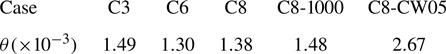
  $\theta$ is shown in table 2 and figure 12. These results suggest that $\theta$ is marginally affected by Mach and Reynolds numbers, showcasing a concentration range between $1.3\times 10^{-3}$ and $1.5\times 10^{-3}$ for Cases C3, C6, C8 and C8-1000. Conversely, wall temperature exerts a more pronounced impact on $\theta$, as evidenced by a significant rise in the cold wall case C8-CW05.
Table 2. Inclination angle  $\theta$ of the leading eigenvector of the inertia tensor $\boldsymbol {I}$.
4.2. Near-wall solenoidal streak density
In incompressible flows, the outer LSMs drive the near-wall streaks to drift in the spanwise direction; however, there lacks obvious correlation between the outer LSMs and the near-wall streak density (Zhou et al. Reference Zhou, Xu and Jiménez2022). Whether this conclusion remains valid for the solenoidal streaks in compressible flows requires further investigation. Hence, we define two spanwise windows, one located at  $y_{1}^+=13$ to capture the near-wall streak density, and the other one at $y=y_{2}$ to obtain the outer large-scale wall-normal velocity, as suggested by Zhou et al. (Reference Zhou, Xu and Jiménez2022). Both windows have the same size $\Delta z$, centred at the same streamwise and spanwise locations. The near-wall streak density $\rho _s$ is computed by counting the local minima of $u_{s}^{(2D)}$, as defined in (4.1a,b). Additionally, $\rho _s=n_s/\Delta z$, where $n_s$ is the number of local minima within the spanwise range $\Delta z$ of the window. The outer large-scale wall-normal velocity, $\widetilde {v_{s}}$, is given by (4.5). Positive $\widetilde {v_{s}}$ represents the up-washing side of the large-scale circulations, with negative $\widetilde {v_{s}}$ for the down-washing side. Here, the window width in the following discussions is chosen to be $\Delta z^+= 214$, the same as that of Zhou et al. (Reference Zhou, Xu and Jiménez2022). The total number of samples used for statistics ranges from $1.99\times 10^{7}$ to $3.32\times 10^{7}$.
The p.d.f. of the near-wall solenoidal streak density is shown in figure 13. Results in Cases C3, C6, C8 and C8-1000 show agreement with the incompressible results, regardless of the Mach numbers and Reynolds numbers, where the p.d.f.s reach their maximum at  $1/\rho _{s}^+\approx 70\sim 85$. This further indicates that the solenoidal streak spacing over adiabatic walls has not undergone significant changes compared with the incompressible flows. However, the cold-wall condition in Case C8-CW05 leads to an increase in the streak spacing, while the peak of the p.d.f.s shifts to $1/\rho _{s}^+\approx 110$.

Figure 13. Probability density function of the streak density at different (a) Mach numbers, (b) Reynolds numbers and wall temperatures. black dashed, the incompressible case at  $Re_{\tau }=550$ of Zhou et al. (Reference Zhou, Xu and Jiménez2022). (a) red, Case C3; blue, Case C6; black, Case C8. (b) black, Case C8; red, Case C8-1000; blue, Case C8-CW05.
The correlation coefficient  $R(\rho _{s},\widetilde {v_{s}})$ is used to quantify the relationship between near-wall solenoidal streak density and outer LSMs, which is defined as
 \begin{equation} R(\rho_{s},\widetilde{v_{s}})=\frac{\displaystyle\sum(\rho_{s}- \bar{\rho_{s}})\tilde{v_{s}}}{\displaystyle\left[\sum(\rho_{s}- \bar{\rho_{s}})^{2}\sum\tilde{v_{s}}^{2}\right]^{{1}/{2}}},\end{equation}
where the mean streak density  $\bar {\rho _{s}^+}\approx 0.01$, and the mean value of $\tilde {v_{s}}$ is $0$. The distributions of the correlation $R(\rho _{s},\tilde {v_{s}})$ at different heights $y_2$ are shown in figure 14. In all cases, the correlation continuously decreases with increasing heights, approaching zero. At different heights, the correlation is consistently smaller than $0.2$, regardless of Mach numbers, Reynolds numbers and wall temperatures. This suggests that, in the compressible flow, there is no obvious accumulation of solenoidal streaks under large-scale circulations, consistent with the conclusion in incompressible turbulent flow.

Figure 14. Correlation  $R(\rho _{s},\tilde {v_{s}})$ between the near-wall streak density $\rho _{s}$ ( $y_1^+=13$) and wall-normal velocity $\tilde {v_{s}}(y_2^+)$ at different (a) Mach numbers, (b) Reynolds numbers and wall temperatures. (a) Case C3, red; Case C6, blue; Case C8, black. (b) Case C8, black; Case C8-1000, red; Case C8-CW05, blue. The dashed black lines denote the correlation $R$ from the incompressible case at $Re_{\tau }=535$ of Zhou et al. (Reference Zhou, Xu and Jiménez2022).
5. Influence of large-scale motions on near-wall dilatational structures
5.1. Streamwise advection velocity of the dilatational structures
Having established the influence of outer LSMs on the near-wall solenoidal streaks, their effects on the dilatational structures remain to be checked. A similar window tracking method as § 4.1 is adopted in this section, to track the spanwise drifting of near-wall dilatational structures. The tracking windows need to follow the dilatational structures in the streamwise direction. Therefore, their mean streamwise advection velocity  $u_{ad}$ shall be discussed first. The method proposed by Kim & Hussain (Reference Kim and Hussain1993) is adopted, where the definition of the correlation $R_{u_{d}}^{x}(\delta x, y, \Delta t)$ is consistent with (4.3). The total number of samples used for statistics ranges from $3.32\times 10^{7}$ to $1.33\times 10^{8}$ in different cases. If the streamwise displacement of $u_{d}$ after $\Delta t$ is $\delta x_{max}$, then $R_{u_{d}}^{x}$ will reach the maximum at $\delta x=\delta x_{max}$. Thus, the mean streamwise advection velocity could be defined as $u_{ad}=\delta x_{max}/\Delta t$.
The streamwise advection velocity of  ${u}_{d}$ at different $\Delta t$ is shown in figure 15. The influence of $\Delta t$ is trivial in the near-wall region $y^+<20$ and outer region $y^+>300$, while $\Delta t$ has a significant effect in the logarithmic region. As suggested in figure 5, $u_{d}$ fluctuations are primarily concentrated in the near-wall and outer regions, rather than the logarithmic region. This indicates the absence of stable dilatational structures in the logarithmic region, where ${u}_{d}$ may experience a stronger dispersion and dissipation, leading to a failure of Taylor's frozen turbulence hypothesis (Taylor Reference Taylor1938). The dilatational structures in the near-wall and outer regions are more stable, and their advection velocity remains robust within the range $\Delta t^+=2.5\sim 10$. In Case C3, ${u}_{ad}^+\approx 16\sim 18$ in the near-wall region, and ${u}_{ad}^+\approx 10\sim 11$ near the channel centre, as shown in figure 15. Both parts are notably different from the advection velocity of solenoidal streaks at the same height.

Figure 15. Wall-normal distributions of the streamwise advection velocity  $u_{ad}$ of ${u}_{d}$ at different $\Delta t$ in Case C3. $\Delta t^+=2.5$, black; $\Delta t^+=5$, red; $\Delta t^+=10$, blue. Two black dashed lines denote $y^+=20$ and $y^+=300$.
It should be noted that  $u_{d}$ is not the sole variable representing the dilatational structures. Therefore, it is essential to consider whether the advection velocities collapse when the dilatational structures are represented by other variables. The dilatational structures are organized in the form of positive and negative fluctuations distributed alternately along the streamwise direction. Motivated by this, Yu et al. (Reference Yu, Liu, Fu, Tang and Yuan2022) applied the streamwise Hilbert transform to $u_{d}$, thereby extracting the envelopes to represent the positions of dilatational structures. Here, we define
 \begin{equation}
u_{H}={abs}({H_{x}}(u_{d})), \quad u_{H+}=\begin{cases}
u_{H} & (u_{H}^+\,{\geq}\,0.12)\\ 0 & (u_{H}^+<0.12)
\end{cases},\end{equation}
\begin{equation}
u_{H}={abs}({H_{x}}(u_{d})), \quad u_{H+}=\begin{cases}
u_{H} & (u_{H}^+\,{\geq}\,0.12)\\ 0 & (u_{H}^+<0.12)
\end{cases},\end{equation}
where the operator  ${H_{x}}$ is the Hilbert transform in the streamwise direction, and $u_{H+}$ is $u_{H}$ filtered with a threshold value of $0.12u_{\tau }$. The instantaneous distributions of ${u}_{d}$ and ${u}_{H}$ are shown in figure 16. The interior regions of the black isolines cover most parts with strong $u_{d}$ fluctuations, indicating that both $u_{H}$ and $u_{H+}$ could represent the dilatational structures.

Figure 16. Instantaneous distributions of  ${u}_{d}$ and ${u}_{H}$ on $(x,z)$ plane at $y^+=10$ (Case C3). Shaded, ${u}_{d}^+$; black contour lines, ${u}_{H}^+=0.12$.
We choose the method proposed by Kim & Hussain (Reference Kim and Hussain1993), similar to (4.3), to calculate the streamwise advection velocity  $u_{ad}$ when selecting different variables to represent the dilatational structures. Results are illustrated in figure 17. The advection velocities of ${u}_{d}$, ${u}_{H}$ and ${u}_{H+}$ are shown in figure 17(a), which are denoted by the slopes of the three lines. Three lines nearly collapse with each other, indicating that the advection velocities using these three variables are approximately the same. Moreover, the advection velocities of the divergence $\theta$ and ${u}_{d}$ are shown in figure 17(b). Although there exist differences between the results of $\theta$ and ${u}_{d}$, the disparities in the near-wall region and the outer region are within the range of $\pm 2u_{\tau }$. In summary, the streamwise advection velocities of stable dilatational structures are similar when represented by different variables. Therefore, $u_{d}$ will be used to represent the dilatational structures in the following discussions.

Figure 17. (a) Positions of maximum correlations  $\delta x_{max}$ in Case C3, as a function of $\Delta t$, when selecting different variables to represent the dilatational structures. ${u}_{d}$, black; ${u}_{H}$, red; ${u}_{H+}$, blue. (b) Wall-normal distributions of the streamwise advection velocity $u_{ad}$ of divergence $\theta$ and dilatational velocity ${u}_{d}$ in Case C3. $\Delta t^+=10$. $\theta$, red; ${u}_{d}$, blue. Two black dashed lines denote $y^+=20$ and $y^+=300$.
Wall-normal distributions of the streamwise advection velocity of  ${u}_{d}$ are shown in figure 18, from different cases. The $u_{ad}$ maintains at $16\sim 18u_{\tau }$ in the near-wall region $y^+<50$, with its value nearly unaffected by the Mach numbers $M_{0}$, Reynolds numbers $Re_{\tau }$ and wall temperature conditions $T_{w}/T_{r}$. This result also collapses with the near-wall advection velocity of pressure fluctuations in incompressible turbulent flows, at approximately $17u_{\tau }$ suggested by Kim & Hussain (Reference Kim and Hussain1993). Thus, $u_{ad}^+=17.0$ will be adopted in § 5.2 when tracking the near-wall dilatational structures. Additionally, the streamwise advection velocity $u_{ad}$ near the channel centre increases with higher Mach numbers, higher Reynolds numbers and colder wall temperatures.

Figure 18. Wall-normal distributions of the streamwise advection velocity  $u_{ad}$ of ${u}_{d}$ at different (a) Mach numbers $M_{0}$, (b) Reynolds numbers $Re_{\tau }$ and wall temperatures $T_{w}/T_{r}$. $\Delta t^+=2.5$. Two black dashed lines denote $y^+=20$ and $y^+=300$. (a) Case C3, red; Case C6, blue; Case C8, black. (b) Case C8, black; Case C8-1000, red; Case C8-CW05, blue.
5.2. Spanwise drift of the near-wall dilatational structures
A window tracking method is adopted to acquire the spanwise drifting velocity of dilatational structures. The near-wall dilatational structures are organized in the form of alternating positive and negative  ${u}_{d}$ along the streamwise direction, with distinct characteristic scales compared with the solenoidal streaks. Consequently, the streamwise-averaged variable $u^{(2D)}$ could not reflect the position of dilatational structures. To quantify the spanwise drifting velocity at a specific point $(t,x_s,y_1,z_s)$, we choose a two-dimensional window to track the dilatational structures, following the PIV method. The correlation $R_{u_{d}}^{z}$ is defined as
 \begin{align} R_{u_{d}}^{z}(\delta
z,\Delta t)&=\frac{1}{(I_{0}I_{1})^{{1}/{2}}}
\int_{x_{s}-\Delta\chi/2}^{x_{s}+\Delta\chi/2}
\int_{z_{s}-\Delta\zeta/2}^{z_{s}+\Delta\zeta/2}u_{d}(t,x,y_{1},z)u_{d}(t+\Delta
t,x\nonumber\\ &\quad +u_{ad}\Delta t,y_{1},z+\delta
z)\,\mathrm{d}z\,\mathrm{d}{\kern0.8pt}x,\end{align}
\begin{align} R_{u_{d}}^{z}(\delta
z,\Delta t)&=\frac{1}{(I_{0}I_{1})^{{1}/{2}}}
\int_{x_{s}-\Delta\chi/2}^{x_{s}+\Delta\chi/2}
\int_{z_{s}-\Delta\zeta/2}^{z_{s}+\Delta\zeta/2}u_{d}(t,x,y_{1},z)u_{d}(t+\Delta
t,x\nonumber\\ &\quad +u_{ad}\Delta t,y_{1},z+\delta
z)\,\mathrm{d}z\,\mathrm{d}{\kern0.8pt}x,\end{align}
where  $I_{0}$ and $I_{1}$ respectively represent the mean squares of $u_{d}(t,x,y_{1},z)$ and $u_{d}(t+\Delta t,x+u_{ad}\Delta t,y_{1},z+\delta z)$, used to normalize the correlation. If the spanwise displacement of the dilatational structures after $\Delta t$ is $\delta z_{max}$, then $R_{u_{d}}^{z}$ will reach its maximum at $\delta z=\delta z_{max}$. Thus, the spanwise drifting velocity at point $(t,x_s,y_1,z_s)$ could be defined as $w_{ad}=\delta z_{max}/\Delta t$. Here, $\Delta \chi$ and $\Delta \zeta$ in (5.2) represent the streamwise and spanwise length of the tracking window, respectively. The window should be short enough to differentiate the dilatational structures from the LSMs, and also long enough to retain the structural information. Here, we choose $\Delta \chi ^+\times \Delta \zeta ^+\approx 200\times 200$. The spanwise length of the window is similar to the scale of the dilatational structures, while the window encompasses one to two pairs of alternating positive and negative fluctuations in the streamwise direction, suggesting this window size is reasonable. Posterior tests show that the results below are robust when $\Delta \chi ^+$ and $\Delta \zeta ^+$ are in the range $150\sim 250$.
The p.d.f. of the spanwise drifting velocity  $w_{ad}$ of near-wall dilatational structures is shown in figure 19. Here, $y_{1}^+=13$ in all cases, and the streamwise advection velocity of the tracking windows is $u_{ad}^+=17.0$. The total number of samples used for statistics ranges from $4.15\times 10^{6}$ to $3.32\times 10^{7}$ in different cases, and points with $R_{u_{d}}^{z}(\delta z_{max})<0.8$ are rejected during the statistics. The drifting velocity is concentrated within the range of $w_{ad}^+=[-4,4]$, exhibiting a broader distribution compared with the $w_{ad}$ of the solenoidal streaks. The influence of different Mach numbers on the distributions of the drifting velocity is minor, as shown in figure 19(a). However, the spanwise drifting of dilatational structures is enhanced with increasing Reynolds numbers and decreasing wall temperatures in figure 19(b). This result suggests that the spanwise drifting of the near-wall dilatational structures may not follow the same mechanism as the streak meandering process.

Figure 19. Probability density function of the drifting velocity  $w_{ad}$ of near-wall dilatational structures at different (a) Mach numbers, (b) Reynolds numbers and wall temperatures. $\Delta t^+=2.5$, $y_{1}^+=13$. (a) Case C3, red; Case C6, blue; Case C8, black. (b) Case C8, black; Case C8-1000, red; Case C8-CW05, blue.
Velocity fluctuations in the outer region are composed of solenoidal and dilatational components, while the dilatational components are significantly smaller than the solenoidal parts in all the cases we discussed, also illustrated in figures 1 and 2. Thus, we focus solely on the large-scale solenoidal components when considering the outer LSMs. The window-filtered wall-normal solenoidal velocity  $\tilde {v_{s}}(x_0,y_2,z_0)$ is used to characterize the LSMs in the outer region, defined by (4.5). The joint p.d.f. of the $w_{ad}$ of near-wall dilatational structures and the outer $\partial \tilde {v_{s}}^+/\partial z^+$ at $y_2^+=150$ in Case C3 is shown in figure 20. The white dashed lines are the statistics from the sample points satisfying $u_{H}^+\geq 0.12$, denoting the more active regions of the dilatational structures. They collapse with the contour levels of the shaded part. It suggests that the continuous $w_{ad}$ field obtained by the PIV method truly represents the drift of the dilatational structures. Although the joint p.d.f. with elliptical contours is preferentially aligned to the first and third quadrants, the elliptical shapes of the contours are closer to being circular, compared with the results from solenoidal streaks in figure 12. This suggests that the influence of outer LSMs on the dilatational structures is notably weaker than their impact on solenoidal streaks.

Figure 20. Joint p.d.f. of the spanwise drift velocity of dilatational structures at  $y_1^+=13$ and $\partial \tilde {v_{s}}^+/\partial z^+$ at $y_2^+=150$ in Case C3. Shaded, $w_{ad}$ by PIV; white dashed lines, $w_{ad}$ from the sample points satisfying $u_{H}^+\geq 0.12$. Contour levels are $0.1$, $0.3$, $0.5$, $0.7$, $0.9$ of the maximum probability density, respectively. $\Delta t^+=2.5$ and $\Delta z^+= 214$.
To quantify the influence of LSMs on the spanwise drifting of near-wall dilatational structures, the correlation coefficient  $R(w_{ad},\partial \tilde {v_{s}}/\partial z)$ is adopted, which is defined as
 \begin{equation} R\left(w_{ad},\frac{\partial\tilde{v_{s}}}{\partial z}\right)=\frac{\displaystyle \sum w_{ad}\left(\dfrac{\partial\tilde{v_{s}}}{\partial z}\right)}{\left[\displaystyle \sum w_{ad}^{2}\sum \left(\dfrac{\partial\tilde{v_{s}}}{\partial z}\right)^{2}\right]^{{1}/{2}}},\end{equation}
where the mean value of  $w_{ad}$ and $\partial \tilde {v_{s}}/\partial z$ is $0$. The distributions of the correlation $R(w_{ad},\partial \tilde {v_{s}}/\partial z)$ at different heights $y_2$ are shown in figure 21. As the height $y_2$ increases, the correlation coefficient $R$ gradually increases, reaching a maximum at approximately $y_{2}^+=100\sim 150$ and then decreases. Results at ${Re}_{\tau }\approx 500$ are similar, with minor influences from Mach numbers and wall temperatures. The maximum value of $R$ is approximately $0.13$, corresponding to the nearly circular ellipses observed in figure 20. It indicates that the influence of LSMs on near-wall dilatational structures is relatively weak at ${Re}_{\tau }\approx 500$. This influence further decreases as ${Re}_{\tau }$ grows to $1000$, as shown by the red dashed line in figure 21. The maximum correlation coefficient is only approximately $0.05$, indicating a trivial influence of outer LSMs. In contrast, the spanwise drifting of dilatational structures is enhanced at ${Re}_{\tau }=1000$ in figure 19(b). This suggests that the influence of outer LSMs is not the primary trigger for the spanwise drifting of dilatational structures.

Figure 21. Correlation  $R(w_{ad},\partial \tilde {v_{s}}/\partial z)$ between the spanwise drift velocity $w_{ad}$ ( $y_1^+=13$) and $\partial \tilde {v_{s}}/\partial z$ at different heights $y_2^+$. Case C3, red; Case C6, blue; Case C8, black; Case C8-1000, red dashed; Case C8-CW05, blue dashed.
Furthermore, a deeper examination is warranted to ascertain the influence of outer dilatational structures on the spanwise drift of near-wall dilatational structures. To this end, we used the correlation coefficient  $R(w_{ad},\partial \tilde {v_{d}}/\partial z)$ as a quantitative measure of this effect, as defined in (5.3). Figure 22 displays the correlation $R(w_{ad},\partial \tilde {v_{d}}/\partial z)$ across various heights $y_2$. The maximal absolute value of $R$ is observed near the wall, roughly $0.1$. With an increase in the height $y_2$, $R$ progressively approaches zero. This indicates that large-scale dilatational structures centred approximately at $y=h$ have trivial effects on the spanwise drift of near-wall dilatational structures across all cases.

Figure 22. Correlation  $R(w_{ad},\partial \tilde {v_{d}}/\partial z)$ between the spanwise drift velocity $w_{ad}$ ( $y_1^+=13$) and $\partial \tilde {v_{d}}/\partial z$ at different heights $y_2^+$. Case C3, red; Case C6, blue; Case C8, black; Case C8-1000, red dashed; Case C8-CW05, blue dashed.
6. Summary and conclusions
The influence of outer large-scale motions (LSMs) on near-wall structures has been investigated in compressible turbulent channel flows. To separate the compressibility effects, this study decomposes the velocity fluctuations into the rotational, solenoidal component and the potential, dilatational component, by employing the Helmholtz decomposition method. The impacts of outer LSMs on the near-wall solenoidal streaks and dilatational structures are considered separately.
The majority of velocity fluctuations in the flow field are contributed by the solenoidal velocity fluctuations, characterized by flow structures including near-wall streaks elongated in the streamwise direction and large-scale structures in the outer region. Their scales, streamwise advection velocities and spanwise meandering characteristics closely resemble those in the incompressible turbulent flows. In compressible flows, the footprint of LSMs penetrating deep into the near-wall region is also observed, with this effect intensifying as the Reynolds number increases. We track the near-wall solenoidal streaks using the particle image velocimetry (PIV) method. Results indicate that the solenoidal streaks drift in the spanwise direction, with velocities of approximately  $\pm u_\tau$, regardless of Mach numbers, Reynolds numbers and wall temperatures. The distribution range of streak drifting velocity is not affected by compressibility, and its magnitude can still be measured using wall units. The drifting velocities in the near-wall region show correlations with the outer wall-normal velocity at large scales. This suggests that in compressible turbulent flows, the outer LSMs still drive the spanwise drifting of the near-wall solenoidal streaks, consistent with the mechanism found in incompressible flows (Zhou et al. Reference Zhou, Xu and Jiménez2022). We also examine the spanwise density of near-wall solenoidal streaks, while the correlations between streak density and outer LSMs are nearly zero. The gathering of solenoidal streaks induced by outer LSMs remains trivial in compressible flows.
Furthermore, the dilatational velocity fluctuations characterize the compressibility effects, corresponding to two main types of flow structures. One consists of small-scale fluctuations alternating along the streamwise direction in the near-wall region, with a scale of approximately  $\lambda _{x}^+\times \lambda _{z}^+=O(100)\times O(400)$. The other comprises isolated large-scale parts located from the outer region to the channel centre, characterized by a scale of approximately $\lambda _{x}\times \lambda _{z}=O(h)\times O(2h)$. The streamwise advection velocity of the dilatational structures exhibits significant differences from the solenoidal streaks. The near-wall advection velocity remains at $16\sim 18u_{\tau }$ in different cases, with trivial influence from Mach number, Reynolds number and wall temperature conditions. We obtain the spanwise drifting velocity of near-wall dilatational structures by employing the PIV method with two-dimensional tracking windows. The spanwise drifting of the near-wall dilatational structures follows a mechanism distinct from the streak meandering process. The drifting velocity is concentrated within the range of $[-4u_{\tau },4u_{\tau }]$, notably larger than the drifting velocity of solenoidal streaks. Furthermore, neither outer LSMs nor large-scale dilatational structures serve as the primary triggers for the spanwise drifting of dilatational structures.
Funding
This work is supported by the National Natural Science Foundation of China (under grant nos. 12272205 and 12388101).
Declaration of interests
The authors report no conflict of interest.


