


1. Introduction
The problem of jet noise reduction continues to motivate both applied and academic research. Since the introduction of jet engines, many studies have been dedicated to this issue (Wirt Reference Wirt1966; Seiner & Krejsa Reference Seiner and Krejsa1989; Saiyed, Bridges & Mikkelsen Reference Saiyed, Bridges and Mikkelsen2000; Ginevsky, Vlasov & Karavosov Reference Ginevsky, Vlasov and Karavosov2004; Morris & McLaughlin Reference Morris and McLaughlin2019; Zigunov, Sellappan & Alvi Reference Zigunov, Sellappan and Alvi2022). But jet noise nonetheless remains one of the main sources of noise at takeoff (Leylekian, Lebrun & Lempereur Reference Leylekian, Lebrun and Lempereur2014; Huff et al. Reference Huff, Henderson, Berton and Seidel2016), and the Advisory Council for Aeronautics Research in Europe (ACARE) has established a goal of reducing perceived noise emissions of aircraft by 65 % by 2050 with respect to noise levels recorded in the year 2000 (European Commission 2011).
Jet noise is the result of mixing the propulsive jet exhaust with the ambient air, and it leads to a broad range of turbulent structures. Among these are what have come to be known as coherent structures (Mollo-Christensen Reference Mollo-Christensen1967; Crow & Champagne Reference Crow and Champagne1971; Lau, Fisher & Fuchs Reference Lau, Fisher and Fuchs1972; Moore Reference Moore1977), which are more acoustically efficient than less-organized components of the turbulence, and dominate downstream sound radiation (Michalke Reference Michalke1983; Tam, Golebiowski & Seiner Reference Tam, Golebiowski and Seiner1996; Tam et al. Reference Tam, Viswanathan, Ahuja and Panda2008). These coherent structures, also known as wavepackets, are underpinned by instability mechanisms; they are characterized by a large spatial envelope of growth and decay, and by a high degree of organization (Gudmundsson & Colonius Reference Gudmundsson and Colonius2011; Jordan & Colonius Reference Jordan and Colonius2013; Cavalieri, Jordan & Lesshafft Reference Cavalieri, Jordan and Lesshafft2019).
When it comes to reducing jet noise, lowering the jet velocity is an obvious possibility, given that the total acoustic power of the jet is roughly proportional to  $U^8$, as predicted by Lighthill (Reference Lighthill1952). Larger engines, developed in the past decades to increase efficiency, result in lower velocity for a given thrust, and this has resulted in substantial reductions of jet noise. But this strategy is reaching its limits due to structural and ground-clearance constraints. Further reduction of jet noise requires new strategies (Leylekian et al. Reference Leylekian, Lebrun and Lempereur2014). One such strategy involves the use of passive devices, such as chevron nozzles (Huff Reference Huff2007; Tide & Srinivasan Reference Tide and Srinivasan2009). Low-frequency noise reduction is produced here thanks to the increase in streamwise vorticity in the shear layer. This enhances mixing, reduces the potential core length, and has a stabilizing effect on Kelvin–Helmholtz wavepackets (Alkislar, Krothapalli & Butler Reference Alkislar, Krothapalli and Butler2007; Sinha et al. Reference Sinha, Gudmundsson, Xia and Colonius2016; Lajús et al. Reference Lajús, Sinha, Cavalieri, Deschamps and Colonius2019). One advantage of such passive control devices is that they do not require an energy input. However, it typically leads to lower thrust efficiency. Another strategy involves the input of external power, by means of an active control scheme, which can be open or closed loop. Open-loop control involves a fixed (steady or harmonic) actuation signal, and the controller does not take into account changes in the flow state. One such approach involves the use of fluidic injection, which has been shown to effectively reduce sound via both steady and unsteady actuation strategies (Castelain et al. Reference Castelain, Sunyach, Juvé and Béra2008; Laurendeau et al. Reference Laurendeau, Jordan, Bonnet, Delville, Parnaudeau and Lamballais2008; Zaman Reference Zaman2010; Maury et al. Reference Maury, Koenig, Cattafesta, Jordan and Delville2012; Kœnig et al. Reference Kœnig, Sasaki, Cavalieri, Jordan and Gervais2016). In closed-loop control, also known as reactive control, strategies, real-time sensor readings are used to drive unsteady actuation; in this case, actuation is determined, via an appropriate control law, by the real-time dynamics of the flow. A reactive control scheme is naturally more challenging to derive and implement, but presents many potential benefits, including the possibility of deriving an optimal control law.
Real-time reactive control has been explored in numerous fluid mechanics problems for both transitional and turbulent flows. Notable examples include control of Tollmien–Schlichting waves (Semeraro et al. Reference Semeraro, Bagheri, Brandt and Henningson2013; Ghiglieri & Ulbrich Reference Ghiglieri and Ulbrich2014; Kotsonis, Shukla & Pröbsting Reference Kotsonis, Shukla and Pröbsting2015), control of channel flow instabilities (Joshi, Speyer & Kim Reference Joshi, Speyer and Kim1997; Högberg, Bewley & Henningson Reference Högberg, Bewley and Henningson2003; Juillet, McKeon & Schmid Reference Juillet, McKeon and Schmid2014), control of flow-induced cavity acoustics (Shaw & Northcraft Reference Shaw and Northcraft1999; Cabell et al. Reference Cabell, Kegerise, Cox and Gibbs2006), control of buffet-flow instability Gao et al. (Reference Gao, Zhang, Kou, Liu and Ye2017), and separation bubble control (Pouryoussefi et al. Reference Pouryoussefi, Mirzaei, Alinejad and Pouryoussefi2016). When it comes to the control of turbulent jets, two different purposes can be observed in the literature: mixing enhancement and attenuation of amplification mechanisms. Mixing enhancement can be obtained by changes in jet dynamics induced by control, which might be of interest, for example, in the improvement of thrust augmentation (Hunter, Presz & Reynolds Reference Hunter, Presz and Reynolds2002) or fuel–air mixing in combustion systems (Smith et al. Reference Smith, Majamaki, Lam, Delabroy, Karagozian, Marble and Smith1997), or to reduce infrared radiation visibility (Knowles & Saddington Reference Knowles and Saddington2006). Examples of application of flow control to enhance jet mixing include Juvet (Reference Juvet1987), Samimy et al. (Reference Samimy, Kim, Kastner, Adamovich and Utkin2007) and Zhou et al. (Reference Zhou, Du, Mi and Wang2012, Reference Zhou, Fan, Zhang, Li and Noack2020). Regarding the attenuation of amplification mechanisms in jets, studies are mostly focused in attenuating flow structures that are responsible for jet noise generation. Within this context, for supersonic jets we can find, for example, the work developed by Zigunov et al. (Reference Zigunov, Sellappan and Alvi2022). For the subsonic case, which is the focus of the present work, a more detailed discussion is presented in what follows.
Given the importance of wavepackets for jet noise, and the fact that their dynamics can be described using linear models, especially near the nozzle exit (Cavalieri et al. Reference Cavalieri, Rodríguez, Jordan, Colonius and Gervais2013), linear control theory appears as an interesting framework for the development of control strategies for jet noise. Samimy et al. (Reference Samimy, Adamovich, Webb, Kastner, Hileman, Keshav and Palm2004) developed one of the first works focused on reactive control of jet. Such work aimed at the development of actuators termed ‘localized arc filament plasma actuators’, where control authority was demonstrated for high-speed jets. Regarding control strategies, Kopiev & Faranosov (Reference Kopiev and Faranosov2008), by means of a two-dimensional model, demonstrated the possibility of suppressing a time-harmonic instability wave of a free shear flow by using an external acoustic excitation with properly chosen amplitude and phase. The approach was later tested experimentally, where harmonically forced disturbances in a turbulent jet were attenuated on one hand by an external acoustic source (Kopiev et al. Reference Kopiev, Belyaev, Zaytsev, Kopiev and Faranosov2013) and later by means of plasma actuation (Kopiev et al. Reference Kopiev2014). This work led to the development of a strategy for controlling natural instability waves in subsonic turbulent jets (Belyaev et al. Reference Belyaev, Bychkov, Zaitsev, Kopiev, Kopiev, Ostrikov, Faranosov and Chernyshev2018), and this was later tested experimentally in a feedback control scheme (Faranosov et al. Reference Faranosov, Bychkov, Kopiev, Kopiev, Moralev and Kazansky2019), where axisymmetric instability waves of a natural jet were attenuated using a plasma actuator placed inside the nozzle, near the exit. In that study, the control was restricted to a single frequency bin, at Strouhal number  $St = 0.46$, and attenuation was achieved for a narrow frequency range around this target frequency. More recently, the inverse feed-forward control (IFFC) method (Sasaki et al. Reference Sasaki, Morra, Fabbiane, Cavalieri, Hanifi and Henningson2018) was used in experimental control studies of band-limited stochastically forced turbulent jets, with the objective of cancelling axisymmetric hydrodynamic wavepackets using synthetic jet actuators (Maia et al. Reference Maia, Jordan, Cavalieri, Martini, Sasaki and Silvestre2021; Maia, Jordan & Cavalieri Reference Maia, Jordan and Cavalieri2022). Several studies were also developed focusing on the control of mixing layers, which can be seen as a simple model for the initial region of the jet shear layer (Wei & Freund Reference Wei and Freund2005; Parezanović et al. Reference Parezanović2014; Shaqarin, Noack & Morzyński Reference Shaqarin, Noack and Morzyński2018).
The IFFC method opened the possibility of controlling disturbances over a broader frequency range, an important step towards the control of a turbulent jet. The IFFC approach involves control laws that are constructed in the frequency domain. When converted back to the time domain, this approach casts the control law as a convolution between sensor readings and a control kernel. However, this convolution may turn out to be non-causal, i.e. it may require future information to construct the present flow actuation. Real-time applications require that only the causal part of the kernel (present and past measurements) be used. In IFFC, this is enforced by truncating the kernel to its causal part. When the anti-causal part of the kernel is negligible, which may be the case where there is sufficient distance between sensors, actuators and targets, the IFFC method can perform similarly to an optimal control approach (Sasaki et al. Reference Sasaki, Morra, Fabbiane, Cavalieri, Hanifi and Henningson2018; Martini et al. Reference Martini, Jung, Cavalieri, Jordan and Towne2022). However, in practice, this is not always possible, as practical constraints may limit sensor and actuator placement; for instance, higher coherence between actuator and sensor signals, on which the success of a linear control strategy depends, are obtained if they are placed close to each other. In this scenario, IFFC kernels have a non-causal part, and truncating the kernel to its causal part results in a substantial degradation of the performance (Brito et al. Reference Brito, Morra, Cavalieri, Araújo, Henningson and Hanifi2021). This issue can be circumvented with the Wiener–Hopf formalism, which provides a framework to compute an optimal control kernel (Martinelli Reference Martinelli2009; Martini et al. Reference Martini, Jung, Cavalieri, Jordan and Towne2022). Recent numerical and experimental studies have shown that Wiener–Hopf-based control can improve the results of IFFC for amplifier flows (Martini et al. Reference Martini, Jung, Cavalieri, Jordan and Towne2022; Audiffred et al. Reference Audiffred, Cavalieri, Brito and Martini2023b). This suggests that turbulent jet control can benefit from the Wiener–Hopf technique as well.
The Wiener–Hopf approach is equivalent to the well-known linear quadratic Gaussian (LQG) method when the same forcing models are used (we refer the reader to Martini et al. (Reference Martini, Jung, Cavalieri, Jordan and Towne2022) for more details). The LQG method is an optimal control approach where the kernel is obtained in the time domain. However, such a method involves the solution of Riccati equations, which typically requires the use of a reduced-order model to lower the degrees of freedom of the system. The Wiener–Hopf method avoids the need for reduced-order models, and allows the direct use of transfer functions educed from experiments.
In the present work, we aim to attenuate axisymmetric hydrodynamic wavepackets in a turbulent jet by means of control laws developed using the Wiener–Hopf approach. We first consider the case of a forced jet. The application of an external forcing increases the amplitudes of the targeted flow structures, making it easier to identify and control them (Crow & Champagne Reference Crow and Champagne1971; Moore Reference Moore1977; Gudmundsson & Colonius Reference Gudmundsson and Colonius2011). This is the same underlying idea as in the work by Maia et al. (Reference Maia, Jordan, Cavalieri, Martini, Sasaki and Silvestre2021). It avoids some of the difficulties of the control of a natural jet, and is a necessary first step to test the control strategy and provide a proof of concept of its suitability. Furthermore, we emphasize that as in Maia et al. (Reference Maia, Jordan, Cavalieri, Martini, Sasaki and Silvestre2021, Reference Maia, Jordan and Cavalieri2022), forcing amplitudes are chosen such that the jet responds linearly. This ensures that the instability mechanisms in the forced jet are essentially the same as in their natural counterparts. In the second part of the study, we extend the control approach to the natural jet case. As highlighted above, this is a more challenging scenario, due to the difficulty in sensing the low-energy axisymmetric wavepackets. A natural jet case is a condition of greater interest since turbulent jets in practice do not involve an explicit forcing.
The characteristics of the control experiment are discussed in the next section. In § 3, the Wiener–Hopf technique is presented briefly, along with the control design considering both the Wiener–Hopf and the IFFC methods. The results obtained by each of these methods are compared and discussed in § 4. Further discussion regarding the control applied and the results obtained is given in § 5, which concludes the paper.
2. Experimental set-up
Real-time flow control experiments of turbulent jets have been performed at the Pprime Institute. We consider jets at Mach number  $0.05$ and Reynolds number $Re = 5 \times 10^4$. Transition to a fully turbulent jet was guaranteed by a strip of carborundum particles placed $2.5D$ upstream of the nozzle exit plane, where $D = 50$ mm is the nozzle diameter. The experimental set-up was based on the experiments reported by Maia et al. (Reference Maia, Jordan, Cavalieri, Martini, Sasaki and Silvestre2021), shown in figure 1. It consisted of six microphones, working as pressure sensors, providing the axisymmetric pressure mode information, which is the input signal $y$ for the control law. The axisymmetric pressure mode obtained for the unforced jet is shown in figure 2. Spectra of the six microphones are very close to each other, indicating azimuthal homogeneity. The axisymmetric mode has only a small fraction of the power, but it is known to be related to the peak acoustic radiation of subsonic jets (Juve, Sunyach & Comte-Bellot Reference Juve, Sunyach and Comte-Bellot1979; Cavalieri et al. Reference Cavalieri, Rodríguez, Jordan, Colonius and Gervais2013).

Figure 1. (a) Sketch of the control scheme of the experimental set-up, showing sensor and actuator positioning (Maia et al. Reference Maia, Jordan, Cavalieri, Martini, Sasaki and Silvestre2021). (b) A side view photo of the control set-up.

Figure 2. Pressure spectra measured by the six microphones and the resulting  $m = 0$ mode. Measurements taken at $x/D = 0.3$ and $r/D = 0.55$.
The actuation  $u$ was provided by synthetic jets generated by a set of six speakers. These actuators work primarily through a blowing and suction process of zero net mass flux that generates a train of vortices moving away from the device's orifice due to self-induced velocity (Wang & Feng Reference Wang and Feng2018). Further downstream, on the jet centreline, a hot wire has been used to take streamwise velocity measurements. The microphones were placed at a distance $x/D = 0.3$ from the nozzle exit, the actuators at a distance $x/D = 1.5$, and the hot wire at $x/D = 2$. The radial distance of the microphones from the jet centreline was $r/D = 0.55$, while the actuators were placed at a radial distance $r/D = 0.7$. These placement choices avoided intrusion of sensors and actuators in the jet plume, such that these remain nonetheless in the near field. The first set of control experiments was performed considering the application of an axisymmetric forcing $d$ provided by synthetic jets generated by a set of eight speakers. The application of a forcing signal helps to improve the coherence between sensors and actuators, and also allows us to compare some of the results obtained here with those obtained by Maia et al. (Reference Maia, Jordan, Cavalieri, Martini, Sasaki and Silvestre2021).
For the forcing, we have considered two configurations of band-limited stochastic signals, one in a Strouhal number range  $0.3 \leq St \leq 0.45$, and the other for $0.3 \leq St \leq 0.85$, with the Strouhal number defined as $St = fD/U$, where $f$ is the oscillating frequency, and $U$ is the jet velocity at the nozzle exit. The actuation was designed in the same Strouhal number range as the forcing, as will be described in the next section. In the case of the unforced (natural) jet, the actuation is within the band $0.3 \leq St \leq 0.85$. This range corresponds, to a great extent, to the most amplified frequencies at the sensor position, due to the Kelvin–Helmholtz mechanism (Maia et al. Reference Maia, Jordan, Cavalieri, Martini, Sasaki and Silvestre2021, Reference Maia, Jordan and Cavalieri2022).
The Simulink tool, which is integrated with MATLAB, has been used to build the control model that was employed in the ControlDesk software from dSPACE, and the MicroLabBox system acquisition from dSPACE has been used for the real-time sensor readings and actuation, following the same procedure as earlier flow control works of our group (Brito et al. Reference Brito, Morra, Cavalieri, Araújo, Henningson and Hanifi2021; Audiffred et al. Reference Audiffred, Cavalieri, Brito and Martini2023b).
3. Control law design
3.1. Overview of the Wiener–Hopf technique
The Wiener–Hopf technique (Noble Reference Noble1958; Martini et al. Reference Martini, Jung, Cavalieri, Jordan and Towne2022) is applied for the jet control problem, and its performance is compared to that of a wave-cancelling approach (Sasaki et al. Reference Sasaki, Morra, Fabbiane, Cavalieri, Hanifi and Henningson2018; Brito et al. Reference Brito, Morra, Cavalieri, Araújo, Henningson and Hanifi2021; Maia et al. Reference Maia, Jordan, Cavalieri, Martini, Sasaki and Silvestre2021). The same control parameters and transfer functions are used for both methods. In this subsection, the Wiener–Hopf technique is presented briefly; further details about this method and its application to control problems can be found in Martini et al. (Reference Martini, Jung, Cavalieri, Jordan and Towne2022). Wiener–Hopf equations are typically associated with problems where a half-domain condition needs to be satisfied, such as a half-convolution problem (Noble Reference Noble1958; Martini et al. Reference Martini, Jung, Cavalieri, Jordan and Towne2022)
 \begin{equation} \int_{0}^{\infty} {{S}}(t-\tau)\,{{W}}_+(\tau) \,{\rm d}\tau= {T}(t), \quad t > 0, \end{equation}
where  ${S}$ and ${T}$ are known functions, and ${{W}}$ is a unknown function (kernel). Since we are dealing with only one reference sensor and one actuator, this is a single-input/single-output control system, thus the variables considered here become scalars. This equation can be extended to $t < 0$ by writing Zich & Daniele (Reference Zich and Daniele2014)
 \begin{equation} \int^{\infty}_ {-\infty} {S}(t-\tau)\,{W_+}(\tau)\,{k}(\tau)\,{\rm d}\tau = {T}(t)\,{k}(t) + {W_-}(t)\,{k}({-}t), \quad {-\infty}< t<\infty, \end{equation}
where  ${k}(t)$ is the Heaviside step function, and ${W_-}(t)$ is an additional unknown function, with the property ${W_-}(t>0)=0$. Taking a Fourier transform leads to
 \begin{equation} {\hat{S}}(\omega)\,{\hat{W}}_+(\omega) = {\hat{W}}_-(\omega)+{\hat{T}(\omega)}, \end{equation}
where  $+$ and $-$ subscripts indicate that the function is analytical in the upper and lower complex half-planes, respectively. This is ensured for ${{W}}_+$ and ${{W}}_-$ as these functions are defined to be zero for negative and positive times, respectively. We may also refer to ${{W}}_+$ and ${{W}}_-$ as causal and anti-causal functions, respectively; these definitions carry over to all $+$ and $-$ functions.
Solution of such a problem can be achieved with multiplicative and additive factorization:
 $$\begin{gather} {\hat{S}}(\omega)= {\hat{S}_-}(\omega)\,{\hat{S}_+}(\omega), \end{gather}$$
 $$\begin{gather}{\hat{S}}_-^{{-}1}(\omega)\,{\hat{T}}(\omega) = ({\hat{S}}_-^{{-}1}(\omega)\, {\hat{T}}(\omega))_+{+} ({\hat{S}}_-^{{-}1}(\omega)\,{\hat{T}}(\omega))_-. \end{gather}$$
 Here, the multiplicative factorization of  ${\hat {S}}(\omega )$ is solved numerically, following Daniele & Lombardi (Reference Daniele and Lombardi2007). With these two factorizations, the solution of (3.1) is given by
 $$\begin{gather} {\hat{W}}_+(\omega) = {\hat{S}}_+^{{-}1}(\omega)\,({\hat{S}}_-^{{-}1}(\omega)\, {\hat{T}}(\omega))_+, \end{gather}$$
 $$\begin{gather}{\hat{W}}_-(\omega) = {\hat{S}}_-(\omega)\,({\hat{S}}_-^{{-}1}(\omega)\,{\hat{T}}(\omega))_-, \end{gather}$$
where  ${\hat {W}}_+$, which is regular in the upper half-complex plane, is the term related to causal control.
3.2. Control law design based on the Wiener–Hopf approach
The Wiener–Hopf based control is considered for a linear dynamical system. An optimal control for such system can be obtained by means of a quadratic cost functional that expresses the control cost and the cost of state deviation from the original condition, with this functional minimized with respect to the control kernel. For simplicity, we first consider a case without feedback contamination i.e. the effect of  $u$ on $y$ is neglected. Causality can be enforced by including Lagrange multipliers $\varLambda _-$ to a quadratic cost functional as
 \begin{equation} J = \int^{\infty}_ {-\infty}(\langle{{{Q}{z^{*}}}{{z}}} + {Ru_+^{*}}{u_+} \rangle )\, {\rm d}t + \int_{-\infty}^{\infty}[{{\varGamma_+}}(t)\,{\varLambda_-}(t)]\,{\rm d}t + \int_{-\infty}^{\infty}[{{\varGamma_+^*}}(t)\,{\varLambda_-^*}(t)]\,{\rm d}t, \end{equation}
where the  $*$ superscript denotes the complex conjugate, ${z}$ is the target for the control problem, $Q$ is a weighting of the state deviation from the original condition, $R$ is a control penalization, ${\varLambda _-}$ is a Lagrange multiplier, $\varGamma$ is the control kernel, and ${u}$ is the actuation signal. As $\varLambda$ is anti-causal, the last two integrals in (3.8) force $\varGamma$ to be causal. A control law $\varGamma$ relates flow measurements $y$ to actuations $u$. In the frequency domain, this relation reads
 \begin{equation} {\hat{u}}(\omega) = {\hat{\varGamma}}(\omega)\,{\hat{y}}(\omega). \end{equation}
We also have that  ${z} = {z_{un}} + {G_{uz}}*{u} = {z_{un}} + {G_{uz}}*{\varGamma *y}$, i.e. the output is a linear combination of the uncontrolled signal and the actuation response, where $z_{un}$ is the uncontrolled signal at the target location, ${G_{uz}}$ is the transfer function from the control signal ${u}$ to the output ${z}$, and $*$ is the convolution operator. For the optimal solutions, (3.8) is minimized with respect to $\varGamma ^*$, yielding the following Wiener–Hopf equation (we refer the reader to Martini et al. Reference Martini, Jung, Cavalieri, Jordan and Towne2022 for details):
 \begin{equation} {\hat{H}_l}{\hat{\varGamma}}_+{\hat{S}_{yy}} + {\hat{\varLambda}}_-{=} {\hat{H}_r}{\hat{S}_{yz}}, \end{equation}
where
 $$\begin{gather} {\hat{H}_l}(\omega) = \hat{G}_{uz}^{*}(\omega)\,{Q}\,{\hat{G}_{uz}}(\omega)+{R}, \end{gather}$$
 $$\begin{gather}{\hat{H}_r}(\omega) ={-}\hat{G}_{uz}^{*}(\omega)\,{Q}. \end{gather}$$
Here,  ${\hat {S}_{yy}}(\omega )$ is the power spectral density (PSD) of the input signal ${y}$, and ${\hat {S}_{yz}}(\omega )$ is the cross-spectral density (CSD) between the observation signal ${y}$ and the target signal ${z}$ without actuation. Applying the factorization presented earlier, the following expression is obtained for ${\hat {\varGamma }}_+$:
 \begin{equation} {\hat{\varGamma}}_+{=} {\hat{S}_{yy\,+}^{{-}1}}({\hat{S}_{yy \,-}^{{-}1}} {\hat{S}_{yz}} {\hat{H}_{r}} {\hat{H}_{l\,-}^{{-}1}})_+ {\hat{H}_{l\,+}^{{-}1}}. \end{equation}
The expression above is thus used for obtaining the optimal causal control law under the Wiener–Hopf formalism (Noble Reference Noble1958; Martinelli Reference Martinelli2009; Martini et al. Reference Martini, Jung, Cavalieri, Jordan and Towne2022).
In the present system, there is a feedback contamination of the sensors  $y$ by the actuators $u$ due to their proximity in the experimental set-up. To account for this, and avoid appearance of a Larson effect (Sanfilippo & Valle Reference Sanfilippo and Valle2013), the Wiener–Hopf kernel is modified as (Martini et al. Reference Martini, Jung, Cavalieri, Jordan and Towne2022)
 \begin{equation} {\hat{\varGamma'}}_+{=} ({{I}}+{\hat{\varGamma}}{\hat{G}_{uy}})^{{-}1}\hat{\varGamma}, \end{equation}
where  ${\hat {G}_{uy}}$ is the transfer function between the actuation signal and the microphone readings.
In the time domain, the actuation shown in (3.9) is given by
 \begin{equation} {u}(t) = \int^{\infty}_{-\infty} {\varGamma}(\tau)\,{y}(t-\tau)\,{\rm d}\tau, \end{equation}
such that with  $\varGamma$ constructed with the Wiener–Hopf approach detailed above, we have $\varGamma (\tau <0)=0$, by construction, i.e. actuations are a function only of previous measurements, thus the control law is causal. This is, however, not the case if causality is not enforced, which requires the integral to be truncated for $\tau >0$ when used for real-time applications. In the following subsections, causal and non-causal kernels will be shown.
3.3. Control law design based on the IFFC method
In the wave-cancelling approach, here also referred to as the IFFC method, the strategy for control involves a direct superposition of the predicted uncontrolled disturbance at the objective position with the actuation. The IFFC control law can be obtained by minimizing a quadratic functional cost, similar to what is shown in (3.8), but without the constraints imposed to obtain a causal kernel, i.e. without the Lagrange multiplier terms, which yields the equation (Sasaki et al. Reference Sasaki, Morra, Fabbiane, Cavalieri, Hanifi and Henningson2018; Brito et al. Reference Brito, Morra, Cavalieri, Araújo, Henningson and Hanifi2021)
 \begin{equation} {\hat{\varGamma}} = \frac{({\hat{G}_{uz}})^{*}{Q}{\hat{G}_{yz}}}{({{\hat{G}_{uz}})^{*}}{Q}({\hat{G}_{uz}})+{R}}, \end{equation}
where  $\hat {G}_{yz}$ is the transfer function between the microphones $y$ and the control target $z$, which is simply ${\hat {S}_{yz}}/{\hat {S}_{yy}}$. Once the inverse Fourier transform of the IFFC kernel is taken, the non-causal part is neglected, i.e. we consider $\varGamma (\tau <0) = 0$ in order to be able to apply the IFFC kernel in experiments.
In order to account for the contamination of the sensor readings caused by the actuators, it is also necessary to take into consideration the transfer function between the actuators and the microphones ( $G_{uy}$). In this case, the IFFC kernel can be obtained as
 \begin{equation} {\hat{\varGamma}} = \frac{({\hat{G}_{uz}} -{\hat{G}_{uy}}{\hat{G}_{yz}})^{*}{Q}{\hat{G}_{yz}}}{({{\hat{G}_{uz}} -{\hat{G}_{uy}}{\hat{G}_{yz}})^{*}}{Q}({\hat{G}_{uz}} -{\hat{G}_{uy}}{\hat{G}_{yz}})+{R}}. \end{equation}
3.4. Further considerations about the control laws
For the present work the CSD and PSD were obtained using the Welch method, using a Hanning window with 218 blocks and 50 % overlap. Since we have used sampling rate  $10$ kHz ( $St = 29.9$) and measurements of $30$ s to identify the transfer functions, we obtained a frequency resolution $11$ Hz ( $St = 0.03$), with a total of $2730$ data points per block.
Some of the energy content captured by the sensors is not related to the axisymmetric mode, including random fluctuations in the flow field, ambient and electrical noise, and also some undesired noise introduced by the actuators and forcing system. In order to prevent this undesired energy content from affecting the kernel, a zero-phase band-pass filter was applied to the raw data before the calculation of the transfer functions. The application of a filter was important because even very-small-amplitude noise in the kernel could result in a significant increase of the actuation amplitudes due to the acoustic feedback contamination. A frequency-based control penalization was used for the control kernels, wherein large penalizations were applied outside the desired frequency band, defined previously. This helps to avoid undesired frequencies that can lead to feedback contamination, and also regularizes the problem, avoiding divisions by zero (or by values close to zero) in (3.13) and (3.16). To further regularize the problem, a noise term of constant value  $1\times 10^{-4}$ was added to the PSD of $u$ and $y$. For the case where a forcing is applied up to Strouhal number $0.85$, better results where obtained using a constant value $1\times 10^{-3}$.
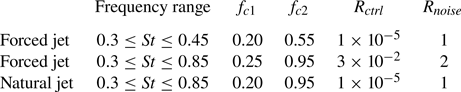
The expressions used to obtain the control penalization are
 $$\begin{gather} R_1 = R_{ctrl} + a(R_{noise}-R_{ctrl})(\tanh(f + f_{c1})-\tanh(f - f_{c1})), \end{gather}$$
 $$\begin{gather}R_2 = R_{ctrl} + a(R_{ctrl} - R_{noise})(\tanh(f + f_{c2})-\tanh(f - f_{c2})), \end{gather}$$
 $$\begin{gather}R=\begin{cases} R_1, & \text{if } f_c \leq (f_{c1} + f_{c2})/2, \\ R_2, & \mathrm{otherwise}, \end{cases} \end{gather}$$
illustrated in figure 3. In the expressions above,  $f$ is the frequency, $f_{c1}$ and $f_{c2}$ are cut-off frequencies, $R_{ctrl}$ defines the penalisation within the region of interest, and $R_{noise}$ is the penalisation out of the region of interest. We have used $a = 30$, a parameter that defines how fast and smooth is the transition from $R_{ctrl}$ to $R_{noise}$. The parameters used in each case are summarized in table 1.

Figure 3. Control penalization as function of the frequency.
Table 1. Parameters considered for the control penalization.
The functions related to the actuation ( ${\hat {G}_{uy}}$ and ${\hat {G}_{uz}}$) were obtained with the forcing off, while $S_{yy}$ and $S_{yz}$ were obtained with the forcing on (for the forced jet cases) and the actuation off. The response of the flow to different amplitudes of actuation and forcing was tested in order to certify that the chosen actuation and forcing amplitudes used to obtain the transfer functions are within the linear range of the flow response. This was verified evaluating the integral of the PSD of the reference sensor $y$ and the target $z$, for various forcing inputs. Figure 4 shows the tests performed for the forced jet case with the control target for $0.3 \leq St \leq 0.45$, where we indicate the amplitudes selected to obtain transfer functions, clearly in a linear range. Figure 4 also indicates that such a linear range is wide for both forcing and actuation. Such linear behaviour is also observed for a broader frequency range, as observed in Maia et al. (Reference Maia, Jordan and Cavalieri2022), with the same experimental set-up considered here.

Figure 4. Response of turbulent jet as functions of actuation and forcing amplitude for the bandwidth  $0.3 \leq St \leq 0.45$, with the indication of the amplitude considered to obtain the transfer functions. The PSD integrals were normalized with respect to the maximal value in the tests.
The magnitude-squared coherence between two signals is a statistical measurement of their degree of linear dependence (Bendat & Piersol Reference Bendat and Piersol2010). The normalized coherence between two signals  $i$ and $j$ is given as
 \begin{equation} \gamma_{ij}^2 = \frac{|\langle S_{ij}\rangle|^2}{|\langle S_{ii}\rangle|\,|\langle S_{jj}\rangle|}, \end{equation}
where  $\langle \cdot \rangle$ is the expectation operator, $S_{ij}$ is the CSD between the pair of signals $i$ and $j$, and $S_{ii}$ and $S_{jj}$ are the PSD functions of signals $i$ and $j$, respectively. The coherences obtained between the sensors and actuators are shown in figure 5. Coherence levels must be sufficiently high for the suitability of the linear control approaches employed here. High coherences indicate a linear relationship between the input and output signals, with low extraneous noise at the input or output signal. Thus higher coherences allow accurate estimates of flow responses.

Figure 5. Coherence between: (a) forcing  $d$ and reference signal $y$; (b) reference signal $y$ and control target $z$; and (c) actuation signal $u$ and control target $z$.
$z$.
As can be observed in the forced jet case, with the increase of the bandwidth, lower coherence levels between the reference sensors and the target were observed for Strouhal numbers below  $0.45$. For $St = 0.37$, for example, $\gamma _{yz}$ dropped by approximately $50\,\%$ with the larger forcing bandwidth. For the forced jet with $0.3 \leq St \leq 0.45$, $\gamma _{yz}$ can also be considered relatively low for $St = 0.34$ and lower, where $\gamma _{yz}$ was below $0.6$. This lower coherence can be explained either by the microphones not being able to properly identify the $m = 0$ structures, e.g. due to azimuthal aliasing, or due to decoherence of the wavepacket along the jet. Unlike transitional flows, characterized by small disturbances, we deal here with a turbulent jet, with coherent structures that nonetheless display an intrinsic coherence decay, imposing additional challenges for flow control. Nevertheless, for the forced jet cases, the coherences between sensors were mostly above $0.8$ for the frequencies of interest. Regarding the natural jet case, low coherence levels were obtained for the entire frequency range considered for control, approximately $0.5$, which makes the control of natural turbulent jets a much more challenging task. The coherence between the actuation signal and the hot wire was higher than $0.85$ for the region of interest, mostly above $0.9$, when considering the forced jet case with $0.3 \leq St \leq 0.45$. However, as the actuation bandwidth increases, lower coherence levels are obtained, which was found to be a limitation of the actuation system. Differences in coherence levels observed between the forced and unforced cases ( $0.3 \leq St \leq 0.85$) can be explained partially by differences in the amplitudes of the actuation signals when identifying the transfer functions, but it was observed that this does not have a significant impact in the obtained kernel. Finally, a very low coherence level can be observed between signals $d$ and $y$ for the unforced jet case. In this case, only electrical noise is captured by the acquisition system, which is not sufficient to activate the forcing system. Thus this low coherence occurs due to imperfect statistical convergence of the coherence, which is expected to go to zero as the number of blocks is increased. Hence the coherences observed between $d$ and $y$ serve as a metric for statistical errors, which are nonetheless low in the present application.
4. Results
4.1. Control kernels
The kernels obtained with the IFFC method and the Wiener–Hopf technique, which were discussed in the previous section, are compared in figures 6 and 7. In practical applications, it is infeasible to apply the non-causal part of the IFFC kernel ( $\tau < 0$) shown in figure 6. For that reason, the non-causal kernel needs to be truncated to its causal part, i.e. we set $\varGamma (\tau < 0) = 0$, which reduces the performance of the controller. The Wiener–Hopf approach provides an optimal truncation strategy, minimizing the performance loss imposed by the causality constraint. The kernels obtained for the natural jet contain oscillations that do not decay to zero, as would be expected (Hervé et al. Reference Hervé, Sipp, Schmid and Samuelides2012; Fabbiane et al. Reference Fabbiane, Simon, Fischer, Grundmann, Bagheri and Henningson2015; Borggaard, Gugercin & Zietsman Reference Borggaard, Gugercin and Zietsman2016; Karban, Martini & Jordan Reference Karban, Martini and Jordan2023); here, they display a harmonic-like signature, due to the peak in $\varGamma ({\omega })$ at approximately $St=0.65$. This is a way for the controller to compensate the low actuator–objective coherence (figure 5c). As the flow has a weak response to actuation for $St\approx 0.65$, in order to attenuate wavepackets at this frequency, a larger control effort becomes necessary. This is thus translated as the transfer function having a strong peak at $St=0.65$, leading to its sine-like behaviour. This behaviour results in the slow decay of $\varGamma (t)$. For the forced jet cases, as the flow is driven by a stochastic signal, the coherent time scales are dominated by the dynamics of forced wavepackets, rather than the intrinsic dynamics of the unforced flow.

Figure 6. Control kernels in the time domain (using dimensionless time, with  $t^* = \tau U/D$) for the forced jets (a) $0.3 \leq St \leq 0.45$ and (b) $0.3 \leq St \leq 0.85$, and (c) for the natural jet (actuation bandwidth $0.3 \leq St \leq 0.85$).

Figure 7. Control kernels in the frequency domain for the forced jets (a)  $0.3 \leq St \leq 0.45$ and (b) $0.3 \leq St \leq 0.85$, and (c) for the natural jet (actuation bandwidth $0.3 \leq St \leq 0.85$).
Wiener–Hopf kernels present higher amplitudes at  $\tau \approx 0$, which is seen as a compensation for the non-causality observed in the IFFC kernels, as the Wiener–Hopf kernel compresses (in an optimal way) the anti-causal part of the IFFC kernel into $\tau = 0$, generating those spikes. As the anti-causal part of the kernel increases by changing actuator or sensor placement, these spikes also increase, as observed in previous works (Martini et al. Reference Martini, Jung, Cavalieri, Jordan and Towne2022; Audiffred et al. Reference Audiffred, Cavalieri, Brito and Martini2023b). Such peaks can also be observed when using the LQG control approach (Morra et al. Reference Morra, Sasaki, Hanifi, Cavalieri and Henningson2020).
When observing the spectra of the kernels in figure 7, one may notice that the energy content of the Wiener–Hopf kernels, for the forced cases, is similar to that of the non-causal ones in the region where the control is designed, while the truncated non-causal solution has considerably lower energy content in this same region, approximately  $70\,\%$ lower for both forced jet conditions. On the other hand, some undesired peaks out of the region of interest appeared for the Wiener–Hopf kernels. That occurs because we are exciting the jet flow with a band-limited stochastic forcing instead of a white noise. Additionally, the raw data are filtered in order to remove some of the energy content present in the region we are not aiming to control, as mentioned earlier. These operations are responsible for the appearance of the peaks. The control penalizations, given by (3.18) and (3.19), prevent these peaks from extending to a larger bandwidth. However, large spectral peaks are still observed. These could be further attenuated by modifying the cut-off frequencies in (3.18) and (3.19), but that would negatively affect the performance of the kernel. In order to demonstrate that the above conditions influence the appearance of the horn-like peaks in the Wiener–Hopf kernels, we consider the following idealized scenario. We set $S_{uy}=0$, consider an artificial white noise actuation signal whose PSD is $S_{uu}$, and assume that the transfer function $G_{uz}$ is given by
 \begin{equation} G_{uz} = {\rm e}^{{\rm i}\omega t_{delay}}, \end{equation}
thus
 \begin{equation} S_{uz} = S_{uu}\,{\rm e}^{{\rm i}\omega t_{delay}}. \end{equation}
In this idealized scenario, the response of the objective sensor  $z$ will be basically the same signal generated by the actuator, but with a delay given by $t_{delay}$, set as $8.6$ ms, which is related to a time delay of the wavepacket excited by actuation in our experiments. All other transfer functions are kept the same as used to obtain the kernels, considering here the case where the control target is limited to $0.3 \leq St \leq 0.45$. From this, we assume four different situations: (i) all the raw data are filtered, as done for the experiments; (ii) no filtering is applied; (iii) filtering is applied for all signals except $u$; (iv) only the actuation signal $u$ is filtered. The kernels obtained, in the frequency domain, are shown in figure 8. One may notice that the horn-like peaks can be suppressed when using a white noise signal for the actuation and avoiding filtering the signals. However, due to limitations in the response of our actuation system, we are constrained to work with band-limited stochastic signals.
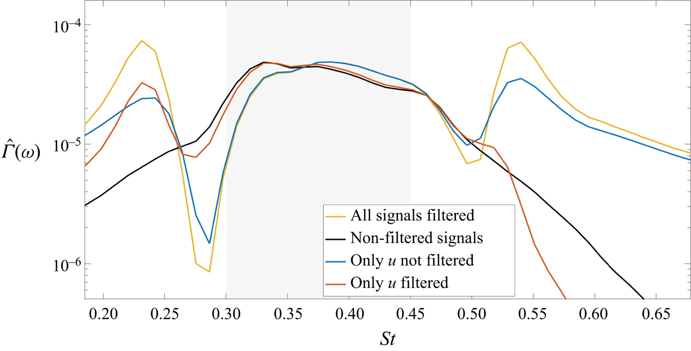
Figure 8. Kernels obtained for an artificial white noise actuation signal considering four different signal processing situations.
4.2. Control results
The control results obtained with the kernels presented above are shown in figure 9, which displays the average PSD of the objective, obtained from three measurements of  $15$ s each, with sampling frequency $10$ kHz. In Audiffred et al. (Reference Audiffred, Cavalieri, Jordan, Martini and Maia2023a), we demonstrated, using this same data set, the control authority, i.e. that the reductions obtained are due to reactive control, not due to changes in the flow dynamics. The same has been demonstrated already by Maia et al. (Reference Maia, Jordan, Cavalieri, Martini, Sasaki and Silvestre2021).

Figure 9. Spectra of the uncontrolled and controlled turbulent jet flows, comparing Wiener–Hopf and IFFC at the control target location, for the kernels obtained for the forced jets (a)  $0.3 \leq St \leq 0.45$ and (b) $0.3 \leq St \leq 0.85$, and (c) the unforced jet, with the control aimed for $0.3 \leq St \leq 0.85$.
For the forced jet cases, a significantly better performance is observed with the Wiener–Hopf kernel in comparison with the IFFC law. Here, the IFFC kernel had a worse performance than reported by Maia et al. (Reference Maia, Jordan, Cavalieri, Martini, Sasaki and Silvestre2021). In the present study, we noticed that the actuator–objective transfer function  $G_{uz}$ was significantly different from that of Maia et al. (Reference Maia, Jordan, Cavalieri, Martini, Sasaki and Silvestre2021). This suggests a difference in actuator placement, or in the intrinsic mechanical characteristics of the actuation system. In any case, the Wiener–Hopf kernel still performed better than what is reported by Maia et al. (Reference Maia, Jordan, Cavalieri, Martini, Sasaki and Silvestre2021). For the case where a forcing is applied for $0.3 \leq St \leq 0.45$, a large peak is observed for the Wiener–Hopf results at Strouhal number approximately $0.52$. Although this is undesired, the peak appears outside the frequency range that we are aiming to control. Recalling that cold jets do not present oscillator behaviour, acting instead as amplifiers (Huerre & Monkewitz Reference Huerre and Monkewitz1990), we understand that this peak is due to the spatial amplification of disturbances introduced at $St \approx 0.52$ by the wave-cancellation kernel, which in the present reactive configuration does not lead to instabilities (Fabbiane et al. Reference Fabbiane, Semeraro, Bagheri and Henningson2014; Schmid & Sipp Reference Schmid and Sipp2016). Accordingly, this undesired peak resulted from one of the peaks observed in the Wiener–Hopf control kernel, as shown in figure 6(a). It is important to note that this is an issue only at narrow actuation bands, due to the filter; the results obtained with larger actuation bandwidths do not show this undesired effect. Furthermore, as the growth rate at this frequency and location is small (Maia et al. Reference Maia, Jordan and Cavalieri2022), the amplification of disturbance is also small and takes place only in the vicinity of the actuator, decaying further downstream, as will be seen in the next subsection. For the case with larger forcing bandwidth, we have observed a considerable increase in the broadband noise outside the frequency range of the excitation signal, which has also been observed in earlier studies (Moore Reference Moore1977; Maia et al. Reference Maia, Jordan, Cavalieri, Martini, Sasaki and Silvestre2021). For the natural jet, similar results were obtained with both control methods considered here, with an attenuation of PSD of approximately $40\,\%$, comparing the uncontrolled and controlled spectra, for the $St$ range of higher amplification of the axisymmetric pressure mode.
4.3. Downstream persistence of control effects
We also verified whether the control effect persisted downstream of the target position for the forced jet case with  $0.3 \leq St \leq 0.45$ and for the natural jet. A significant attenuation of the signals could still be observed until the streamwise position $x/D = 7$, as shown in figures 10 and 11. For the forced case, we can observe that the Wiener–Hopf approach had a more positive impact for frequencies closer to the upper limit of the targeted frequency range compared to the IFFC approach, such that no forcing effect is visible for the Wiener–Hopf results at $x/D = 7$. For the natural jet, reductions of approximately $25\,\%$ can be observed in the velocity spectra at $x/D = 7$, showing that control benefits are not restricted to the target location. It is also important to notice that the peak appearing outside the frequency range aimed at by the control, mentioned earlier, decays quickly as we move downstream.

Figure 10. Spectra of the uncontrolled and controlled forced jet flows ( $0.3\leq St\leq 0.45$) at different positions in the streamwise direction: (a) $x/D = 2.5$, (b) $x/D = 5$, (c) $x/D = 6$, (d) $x/D = 7$.
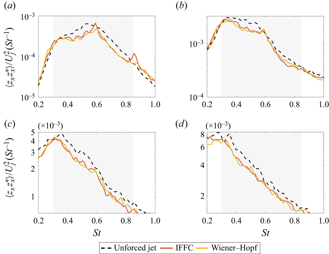
Figure 11. Spectra of the uncontrolled and controlled natural jet flows at different positions in the streamwise direction: (a)  $x/D = 2.5$, (b) $x/D = 5$, (c) $x/D = 6$, (d) $x/D = 7$.
4.4. Control of unforced jet: improvement on sensor placement
As observed in figure 5, the coherence between sensors drops significantly in the absence of a forcing applied to the jet. Since the amplitude of wavepackets increases as they are convected by the jet, it becomes easier to detect them. Thus in order to seek larger attenuations for the unforced jet case, we considered positioning the array of microphones at a slightly downstream position, at  $x/D = 0.58$, remaining nonetheless close to the nozzle. With this, we also changed the radial position of the sensors, moving them to $r/D =0.6$, due to the thicker shear layer at that position. A comparison between the coherence between the target sensor $z$ and the two positions of $y$ sensors is shown in figure 12, confirming that the downstream $y$-sensor placement leads to higher coherence and thus better estimation capabilities.

Figure 12. Coherence between the microphones and the hot wire, comparing the cases with the microphones at  $x/D = 0.3$ and at $x/D = 0.58$.
Since the coherence is still low for  $St<0.45$, we decided to restrict the actuation signal to the range $0.45 \leq St \leq 0.9$. The kernels for these new conditions are shown in figure 13. With this higher coherence, the obtained kernels display a stronger decay over time, as usual in flow control applications (Hervé et al. Reference Hervé, Sipp, Schmid and Samuelides2012; Fabbiane et al. Reference Fabbiane, Simon, Fischer, Grundmann, Bagheri and Henningson2015; Borggaard et al. Reference Borggaard, Gugercin and Zietsman2016; Karban et al. Reference Karban, Martini and Jordan2023).

Figure 13. Control kernels of the unforced jet with the sensors farther downstream, in (a) the time domain and (b) the frequency domain.
The spectra of the uncontrolled and controlled signals obtained with these new kernels are presented in figure 14 for the objective position and in figure 15 for measurements taken farther downstream. With the Wiener–Hopf kernel, at the objective position, reductions of more than  $60\,\%$ of PSD could be obtained for the most amplified frequencies. A similar attenuation could also be obtained with the IFFC kernel; however, a much worse performance is observed at Strouhal number approximately $0.58$. We also considered here an open-loop actuation case, where the actuators provide a band-limited stochastic signal with the same frequency range target as the reactive control, from where it can be noticed that a simple open-loop actuation does not lead to attenuation of wavepackets, amplifying instead coherent turbulent structures. This highlights that the reductions of spectra by Wiener–Hopf and IFFC are due to real-time control effects.

Figure 14. Spectra of the uncontrolled and controlled turbulent jet flows, comparing Wiener–Hopf and IFFC at the control target location.

Figure 15. Spectra of the uncontrolled and controlled turbulent jet flows (for  $y$ at $x/D = 0.58$), at different positions in the streamwise direction: (a) $x/D = 2.5$, (b) $x/D = 5$, (c) $x/D = 6$, (d) $x/D = 7$.
When the reference sensors get closer to the actuators, the non-causal part of IFFC kernels increases, which deteriorates the performance of the truncated kernel, as reported in Martini et al. (Reference Martini, Jung, Cavalieri, Jordan and Towne2022) and Audiffred et al. (Reference Audiffred, Cavalieri, Brito and Martini2023b). The worse performance of the IFFC kernel at Strouhal number approximately  $St = 0.58$ seems also to be related to the low coherence presented by the actuator for this same region (figure 5), whereas the Wiener–Hopf kernel was able to compensate for that, by taking into account the non-causality characteristic of the IFFC kernel, and generating an overall stronger actuation benefit.
We also evaluated the overall performance of the kernels, at different streamwise positions, in terms of the root mean square (RMS) of velocity fluctuations of the controlled and uncontrolled signals. The result of this, for the unforced case with the sensors further downstream, is shown in figure 16. The Wiener–Hopf kernel could provide a reduction of  $28\,\%$ of the RMS of the velocity fluctuations at the target location, which represents an overall reduction of $50\,\%$ of the PSD. On the other hand, the IFFC approach provided an RMS reduction of $12\,\%$. The performance of the IFFC kernel reaches a peak at $x/D = 4$, with an RMS reduction of $16\,\%$. Farther downstream, we observe a linear decay of the control effect.

Figure 16. Relative performance of the control kernels for the unforced jet case, in terms of the RMS of velocity fluctuations of the controlled signals at different positions.
5. Conclusion
This work demonstrates, experimentally, the reactive control of turbulent jets, where a Wiener–Hopf approach is used to obtain the control kernels, and the performance of the controller is compared with that of an inverse feed-forward control (IFFC) method. The control law aims to attenuated axisymmetric coherent structures associated with linear growth mechanisms, which are known to be important for jet noise (Jordan & Colonius Reference Jordan and Colonius2013). The Wiener–Hopf-based control improves on previous results reported by Maia et al. (Reference Maia, Jordan, Cavalieri, Martini, Sasaki and Silvestre2021) for turbulent jets forced stochastically. And we extend the control experiments to unforced jets; this is the first time, to the best of our knowledge, that reactive control is performed on unforced turbulent jets. Attenuations of up to  $60\,\%$ in fluctuation energy were obtained in the unforced case. The control effect was found to persist well downstream of the control target location, for both the forced and unforced cases.
The study was motivated by results obtained in previous work, where the Wiener–Hopf technique was used for flow control, both numerically (Martini et al. Reference Martini, Jung, Cavalieri, Jordan and Towne2022) and experimentally (Audiffred et al. Reference Audiffred, Cavalieri, Brito and Martini2023b), and in other work where stochastically forced jets were controlled using the IFFC method (Brito et al. Reference Brito, Morra, Cavalieri, Araújo, Henningson and Hanifi2021; Maia et al. Reference Maia, Jordan, Cavalieri, Martini, Sasaki and Silvestre2021). A key contribution of the present work, with respect to those mentioned, is the application to an unforced turbulent shear flow where coherence levels between sensor/actuator and objective, essential for the construction of an effective control law, are considerably lower than in forced or pre-transitional flows.
Sensor position was shown to constitute an important parameter. Displacement of the sensors from  $x/D = 0.3$ to $x/D = 0.58$ led to better coherence levels with the downstream target sensor, and with this, the attenuation of turbulence levels was improved accordingly. In this context, the Wiener–Hopf technique played a major role insofar as it permitted the non-causal part of the kernel – which becomes important in the IFFC approach as sensor and actuator are moved closer together – to be suppressed appropriately; in this scenario, the optimal, causal, Wiener–Hopf controller significantly outperforms the IFFC controller. In this case, a reduction of $28\,\%$ of the velocity fluctuations was achieved in terms of RMS, and an associated target frequency range integrated energy reduction of $50\,\%$.
Although this control experiment was performed for low Mach number, the control of a natural turbulent jet presented here is an important step towards the control of turbulent jets in real flight conditions. Furthermore, the same sound generation mechanisms are observed for higher Reynolds numbers and Mach numbers, with sound radiation for low polar angles dominated by the axisymmetric mode (Cavalieri et al. Reference Cavalieri, Jordan, Colonius and Gervais2012). It is important to note that the jet is initially turbulent. Furthermore, the underpinning linear instability mechanisms are essentially inviscid. Thus higher Reynolds numbers are not expected to significantly affect the flow regime or fundamentally change the result. The main change would be a change in the convection velocity caused by increased velocity of the jet, which means that the controller would need to adapt the wavepacket phase accordingly. This statement is also supported by the work developed by Samimy et al. (Reference Samimy, Webb, Esfahani and Leahy2023), who showed that a high-Reynolds-number compressible jet displays similar dynamics to its lower-Reynolds-number counterpart. It would be interesting, nonetheless, to adapt the current approach with considerations of robustness, to enable the controller to adapt to changes in flow conditions. This will be the objective of future studies. With such improvements, and improvements in actuation technology, the control strategy adopted here may be extended to higher Mach numbers, and open perspectives for technological applications. For future work, we also suggest the extension to helical azimuthal modes not explored in this work. This could be undertaken via a multiple input, multiple output approach such as has been successful in boundary layer control (Fabbiane, Bagheri & Henningson Reference Fabbiane, Bagheri and Henningson2017; Sasaki et al. Reference Sasaki, Morra, Cavalieri, Hanifi and Henningson2019; Morra et al. Reference Morra, Sasaki, Hanifi, Cavalieri and Henningson2020).
Acknowledgements
We acknowledge the technical support provided by A. Lebedev, who greatly assisted in the experiments conducted for this work.
Funding
This work has received funding from the European Union's Horizon 2020 research and innovation programme under grant agreement no. 861438. We also wish to acknowledge the financial support from Coordination for the Improvement of Higher Education Personnel (CAPES) and from the São Paulo Research Foundation (FAPESP), grants 2022/03279-5 and 2019/26546-6.
Declaration of interests
The authors report no conflict of interest.


