2.1. Linear solutions

To obtain the dispersion relation, we consider perturbations with wavenumber $k=2{\rm \pi} /\lambda$ of the form

(2.11a,b)$$\begin{gather} \eta^{-} = \epsilon K\,{\mathrm e}^{{{\mathrm i}}kx}+\text{c.c.}, \quad \eta^{+} = \epsilon L\,{\mathrm e}^{{{\mathrm i}}kx}+\text{c.c.}, \end{gather}$$

(2.12)$$\begin{gather}\phi_{1} ={-}x+\epsilon P\cosh(k(\kern0.7pt y+h_1+1/2))\,{\mathrm e}^{{{\mathrm i}}kx}+\text{c.c.}, \end{gather}$$

(2.13)$$\begin{gather}\phi_{2} ={-}x+\epsilon (Q\cosh(k(\kern0.7pt y+1/2))+S\cosh(k(\kern0.7pt y-1/2)))\,{\mathrm e}^{{{\mathrm i}}kx}+\text{c.c.}, \end{gather}$$

(2.14)$$\begin{gather}\phi_{3} ={-}x+\epsilon T\cosh(k(\kern0.7pt y-h_3-1/2))\,{\mathrm e}^{{{\mathrm i}}kx}+\text{c.c.}, \end{gather}$$

(2.15a,b)$$\begin{gather}B^-= (1-R_1)(1-1/F^2),\quad B^+= (R_3-1)(1+1/F^2), \end{gather}$$

where $K, L, P, Q, S$ and $T$ are constant coefficients, c.c. denotes a complex conjugate and $\epsilon$ is a small parameter to measure the nonlinearity. The $-x$ term in the velocity potentials $\phi _i$ corresponds to the uniform stream of speed unity, arising due to the moving frame of reference. Substituting the above quantities into (2.4)–(2.7) and collecting terms of $O (\epsilon )$, we can get six homogeneous linear equations for $K$, $L$, $P$, $Q$, $S$ and $T$. Using the solvability condition, we can obtain a fourth-order algebraic equation of $F$:

(2.16)\begin{equation} \mathcal{A} F^4+\mathcal{B} F^2+\mathcal{C} = 0, \end{equation}

where the coefficients are

(2.17)$$\begin{gather} \mathcal{A} = k^2[ 1+\coth(k) (R_1 \coth(kh_1)+R_3 \coth(k h_3)) +\coth(kh_1)\coth(kh_3)R_1R_3 ], \end{gather}$$

(2.18)$$\begin{gather}\mathcal{B} = k[ \coth(k)(R_3-R_1)+R_3\coth(kh_3)(1-R_1)-R_1\coth(kh_1)(1-R_3)], \end{gather}$$

(2.19)$$\begin{gather}\mathcal{C} = R_3+R_1-R_3R_1-1. \end{gather}$$

Solving this equation for the positive roots, we obtain the following two branches of the dispersion relation:

(2.20a,b)\begin{equation} F_1 = c_{p1}(k,R_1,R_3,h_1,h_3), \quad F_2 = c_{p2}(k,R_1,R_3,h_1,h_3), \end{equation}

where $c_{p1}\ge c_{p2}$ for the same parameters (a rigorous proof that $F^2>0$ can be found in Yih (Reference Yih2012), which applies to Euler multilayer fluids). Here $c_{p1}$ and $c_{p2}$ are the phase velocities of the mode-1 and the mode-2 waves. Mode-1 waves are defined by interface displacements of the same polarity ($KL>0$) and mode-2 waves have interface displacements of opposite polarity ($KL<0$). These linear solutions will be used as initial guesses to generate fully nonlinear profiles, and to motivate certain resonances between modes.

3.1. Boundary integral equations

For periodic waves having a wavenumber $k$, we introduce the following transformation:

(3.1)\begin{equation} \zeta = {\mathrm e}^{-{{\mathrm i}} kz}, \end{equation}

where $z = x+{\mathrm i} y$. This maps the physical region in one spatial period to an annular region in the $\zeta$-plane and enables us to apply Cauchy's integral formula to solve the Laplace equation. Introducing the complex velocity $w = u-{{\mathrm i}} v$, where $u$ and $v$ are the horizontal and vertical components of the velocity, we have the following Cauchy's integral formula on the $\zeta$-plane:

(3.2)\begin{equation} w(\zeta') = \frac{1}{{{\mathrm i}}{\rm \pi}}\oint_C\frac{w(\zeta)}{\zeta-\zeta'}\,{\mathrm d}\zeta,\end{equation}

where $\zeta$ and $\zeta '$ are points on the boundary $C$ of each fluid layer on which the integral is evaluated. Note that the integral has a singularity when $\zeta =\zeta '$, therefore, the integral is in the sense of Cauchy principal value. We can express the complex velocity $w$ in terms of the velocity modulus $q$ and the inclination angle $\theta$ as

(3.3)\begin{equation} w = q\,{\mathrm e}^{-{{\mathrm i}}\theta}. \end{equation}

On the interface, $\theta$ has the following relation to $z$:

(3.4)\begin{equation} \frac{\mathrm{d}z}{\mathrm{d}s} = {\mathrm e}^{{{\mathrm i}}\theta},\end{equation}

where $s$ is the physical arclength parameter and we require that $s$ is monotonically increasing along the interfaces in the direction such that the relatively heavier fluid is always to the right of the interfaces. In this way, (3.2) can be rewritten as

(3.5)\begin{equation} w(s') ={-}\frac{k}{\rm \pi}\oint_C\frac{q(s)}{1-\zeta(s')/\zeta(s)}\,{\mathrm d}s, \end{equation}

where we have used (3.4). For the lower and the upper layer, (3.5) requires the information on the solid walls. However, using the Schwarz reflection principle, we can avoid this by reflecting the lower (upper) interface with respect to the bottom (top) wall to get a mirror image. In this fashion, the solid boundaries become a flat streamline inside the new region of the lower and upper layer, and (3.5) can be calculated by evaluating the integral on the physical interface and its mirror image. In the lower fluid layer,

(3.6)\begin{equation} \zeta(s')/\zeta(s) = \left\{ \begin{array}{@{}ll} {\mathrm e}^{-{{\mathrm i}}k(x'-x)}\, {\mathrm e}^{k(\eta^{-'}-\eta^{-})}, & \text{on the lower interface}, \\ {\mathrm e}^{-{{\mathrm i}}k(x'-x)}\, {\mathrm e}^{k(\eta^{-'}+\eta^{-}+2h_1)}, & \text{on the image of lower interface;} \end{array} \right. \end{equation}

in the upper layer,

(3.7)\begin{equation} \zeta(s')/\zeta(s) = \left\{ \begin{array}{@{}ll} {\mathrm e}^{-{{\mathrm i}}k(x'-x)}\, {\mathrm e}^{k(\eta^{+'}-\eta^{+})}, & \text{on the upper interface}, \\ {\mathrm e}^{-{{\mathrm i}}k(x'-x)}\, {\mathrm e}^{k(\eta^{+'}+\eta^{+}-2h_3)}, & \text{on the image of upper interface;} \end{array} \right. \end{equation}

on the lower interface of the middle layer,

(3.8)\begin{equation} \zeta(s')/\zeta(s) = \left\{ \begin{array}{@{}ll} {\mathrm e}^{-{{\mathrm i}}k(x'-x)}\, {\mathrm e}^{k(\eta^{-'}-\eta^{-})}, & \text{on the lower interface} ,\\ {\mathrm e}^{-{{\mathrm i}}k(x'-x)}\, {\mathrm e}^{k(\eta^{-'}-\eta^{+}-1)}, & \text{on the upper interface;} \end{array} \right. \end{equation}

on the upper interface of the middle layer,

(3.9)\begin{equation} \zeta(s')/\zeta(s) = \left\{ \begin{array}{@{}ll} {\mathrm e}^{-{{\mathrm i}}k(x'-x)}\, {\mathrm e}^{k(\eta^{+'}-\eta^{-}+1)}, & \text{on the lower interface}, \\ {\mathrm e}^{-{{\mathrm i}}k(x'-x)}\, {\mathrm e}^{k(\eta^{+'}-\eta^{+})}, & \text{on the upper interface.} \end{array} \right. \end{equation}

Finally, we can obtain four boundary integral equations by taking the imaginary part of (3.5),

(3.10)$$\begin{gather} q_1(s')\sin(\theta^-(s')) = \frac{k}{\rm \pi}\underbrace{\int_{-\alpha^-}^{\alpha^-}{\rm Im}\left( \frac{q_1(s)}{1-\dfrac{\zeta(s')}{\zeta(s)}} \right)\,{\mathrm d}s}_{\text{mirror image of lower interface}} - \frac{k}{\rm \pi}\underbrace{\int_{-\alpha^-}^{\alpha^-}{\rm Im}\left( \frac{q_1(s)}{1-\dfrac{\zeta(s')}{\zeta(s)}} \right)\,{\mathrm d}s}_{\text{lower interface}}, \end{gather}$$

(3.11)$$\begin{gather}q_2^-(s')\sin(\theta^-(s')) = \frac{k}{\rm \pi}\underbrace{\int_{-\alpha^-}^{\alpha^-}{\rm Im}\left( \frac{q_2^-(s)}{1-\dfrac{\zeta(s')}{\zeta(s)}} \right)\,{\mathrm d}s}_{\text{lower interface}} - \frac{k}{\rm \pi}\underbrace{\int_{-\alpha^+}^{\alpha^+}{\rm Im}\left( \frac{q_2^+(s)}{1-\dfrac{\zeta(s')}{\zeta(s)}} \right)\,{\mathrm d}s}_{\text{upper interface}}, \end{gather}$$

(3.12)$$\begin{gather}q_2^+(s')\sin(\theta^+(s')) = \frac{k}{\rm \pi}\underbrace{\int_{-\alpha^-}^{\alpha^-}{\rm Im}\left( \frac{q_2^-(s)}{1-\dfrac{\zeta(s')}{\zeta(s)}} \right)\,{\mathrm d}s}_{\text{lower interface}} - \frac{k}{\rm \pi}\underbrace{\int_{-\alpha^+}^{\alpha^+}{\rm Im}\left( \frac{q_2^+(s)}{1-\dfrac{\zeta(s')}{\zeta(s)}} \right)\,{\mathrm d}s}_{\text{upper interface}}, \end{gather}$$

(3.13)$$\begin{gather}q_3(s')\sin(\theta^+(s')) = \frac{k}{\rm \pi}\underbrace{\int_{-\alpha^+}^{\alpha^+}{\rm Im}\left( \frac{q_3(s)}{1-\dfrac{\zeta(s')}{\zeta(s)}} \right)\,{\mathrm d}s}_{\text{upper interface}} - \frac{k}{\rm \pi}\underbrace{\int_{-\alpha^+}^{\alpha^+}{\rm Im}\left( \frac{q_3(s)}{1-\dfrac{\zeta(s')}{\zeta(s)}} \right)\,{\mathrm d}s}_{\text{mirror image of upper interface}}, \end{gather}$$

where $2\alpha ^-$ and $2\alpha ^+$ are the total arclength in a spatial period for the lower and upper interfaces, $q_1$ and $q_3$ are the tangential velocities of the lower and upper fluid layers on their corresponding interfaces, $q_2^-$ and $q_2^+$ are the tangential velocities of the middle fluid layer on the lower and the upper interfaces, and $\theta ^-$ and $\theta ^+$ are the inclination angles of the lower and upper interfaces. Note that we have put the point where $s=0$ on the symmetry axis, i.e. the $y$-axis.

3.2. Fourier series solutions

For the convenience of numerical calculation, we introduce two pseudoarclength parameters $\tau ^{\pm }= s/\alpha ^{\pm }\in [-1,1]$ and write the following Fourier series of the six unknown functions:

(3.14a–c)$$\begin{gather} q_1 = \sum_{n=0}^{\infty} a_n \cos(n{\rm \pi} \tau^-),\quad q_2^{-} = \sum_{n=0}^{\infty} b_n \cos(n{\rm \pi} \tau^-),\quad q_2^{+} = \sum_{n=0}^{\infty} c_n \cos(n{\rm \pi} \tau^+), \end{gather}$$

(3.15a–c)$$\begin{gather}q_3 = \sum_{n=0}^{\infty} d_n \cos(n{\rm \pi} \tau^+),\quad \theta^{-} = \sum_{n=1}^{\infty} e_n \sin(n{\rm \pi} \tau^-),\quad \theta^{+} = \sum_{n=1}^{\infty} f_n \sin(n{\rm \pi} \tau^+). \end{gather}$$

Using (3.4), we can construct the lower and upper interfaces from $\theta ^-$ and $\theta ^+$ by the following equations:

(3.16a,b)$$\begin{gather} x^{-}(\tau^-) = \alpha^-\int_{0}^{\tau^-}\cos(\theta^{-}(\tau))\,{\mathrm d}\tau,\quad \eta^{-}(\tau^-) = \eta^{-}_{0} + \alpha^-\int_{0}^{\tau^-}\sin(\theta^{-}(\tau))\,{\mathrm d}\tau, \end{gather}$$

(3.17a,b)$$\begin{gather}x^{+}(\tau^+) = \alpha^+\int_{0}^{\tau^+}\cos(\theta^{+}(\tau))\,{\mathrm d}\tau,\quad \eta^{+}(\tau^-) = \eta^{+}_{0} + \alpha^+\int_{0}^{\tau^+}\sin(\theta^{+}(\tau))\,{\mathrm d}\tau, \end{gather}$$

in which $\eta ^{\pm }_{0}$ are unknowns. To guarantee spatial periodicity that $x^{\pm }(\tau ^{\pm })|_{0}^1=2{\rm \pi} /k$, we must impose the following conditions:

(3.18)\begin{equation} \alpha^-\int_{{-}1}^{1}\cos(\theta^{-}(\tau^-))\,{\mathrm d}\tau^-= \alpha^+\int_{{-}1}^{1}\cos(\theta^{+}(\tau^+))\,{\mathrm d}\tau^+= \frac{2{\rm \pi}}{k}.\end{equation}

To determine $\eta _0^{\pm }$, we need to impose the following constraints which represent volume conservation:

(3.19)\begin{equation} \int_{0}^{1}\eta^{-}\frac{{{\rm d}\kern0.7pt x}^{-}}{{\mathrm d}\tau^-}\,{\mathrm d}\tau^-= \int_{0}^{1}\eta^{+}\frac{{{\rm d}\kern0.7pt x}^{+}}{{\mathrm d}\tau^+}\,{\mathrm d}\tau^+= 0.\end{equation}

Also, we need to prescribe the current speed $-c$ (which has been scaled to $-1$) defined as the average velocity in the lower fluid

(3.20)\begin{equation} \frac{k}{2{\rm \pi}}\int_{-{\rm \pi}/k}^{{\rm \pi}/k} u_1(x,y=\text{const.})\,{{\rm d}\kern0.7pt x} ={-}1,\end{equation}

where $y = \text {const.}$ is an arbitrary horizontal line within the lower layer. Equation (3.20) can be rewritten in terms of $q_1$ using the irrotationality condition

(3.21)\begin{equation} \frac{k}{2{\rm \pi}}\int_{-\alpha^-}^{\alpha^-} q_1(s)\,{\mathrm d}s ={-}1.\end{equation}

In addition, similar conditions for the middle and upper layers are also necessary. Here we focus on the case that all three layers have the same averaged background current (implying zero average shear between each layer). Therefore, the same condition as in (3.21) is adopted for $q_2^-$, $q_2^+$ and $q_3$. Using the pseudoarclength parameters, we have the following four conditions:

(3.22)\begin{equation} \frac{\alpha^- k}{2{\rm \pi}}\int_{{-}1}^{1} q_{1}\,{\mathrm d}\tau^-= \frac{\alpha^- k}{2{\rm \pi}}\int_{{-}1}^{1} q_{2}^{-}\,{\mathrm d}\tau^-=\frac{\alpha^+ k}{2{\rm \pi}}\int_{{-}1}^{1} q_{2}^{+}\,{\mathrm d}\tau^+= \frac{\alpha^+ k}{2{\rm \pi}}\int_{{-}1}^{1} q_{3}\,{\mathrm d}\tau^+= -1. \end{equation}

These conditions imply the following equations:

(3.23a,b)\begin{equation} a_0 = b_0 ={-}\frac{\rm \pi}{\alpha^- k},\quad c_0 = d_0 ={-}\frac{\rm \pi}{\alpha^+ k}. \end{equation}

3.3. Newton's method for the nonlinear system

Since we focus on waves which have symmetry about the $y$-axis, only half of the spatial period is needed in the computation. Therefore, we introduce $N$ uniformly distributed mesh points $\tau ^{\pm }_n$ in the right half-interval $[0,1]$:

(3.24)\begin{equation} \tau^{{\pm}}_{n} = \frac{n-1}{N-1}, \quad n = 1,2,\ldots,N. \end{equation}

To avoid the singularity in the integral equations, we introduce a second set of mesh points $\tau ^{m\pm }_{n}$:

(3.25)\begin{equation} \tau^{m\pm}_{n} = \frac{\tau^{{\pm}}_{n}+\tau^{{\pm}}_{n+1}}{2}, \quad n = 1,2,\ldots,N-1. \end{equation}

We let the boundary integral equations (3.10)–(3.13) to be satisfied on $\tau _n^{m\pm }, n = 1,2,\ldots,N-1$. The integrals are calculated by the trapezoid rule using the function values on $\tau _n, n=1,2,\ldots, N$, which gives a spectral accuracy for periodic functions. The Bernoulli equations (2.4) and (2.5) are rewritten as

(3.26)$$\begin{gather} (q_2^{-})^2 - R_1 q_1^2 + \frac{2(1-R_1)}{F^2}\left(-\frac12 +\eta^-\right) = B^-, \end{gather}$$

(3.27)$$\begin{gather}R_3 q_3^2 -(q_2^+)^2 + \frac{2(R_3-1)}{F^2}\left(\frac12 +\eta^+\right) = B^+, \end{gather}$$

and satisfied on $\tau _n, n = 1,2,\ldots,N$. Together with the four conditions (3.18), (3.19), we have $6N$ equations to solve. To close the system, we truncate the Fourier series after $N$ terms to get $6(N-1)$ unknown coefficients $a_n,b_n,c_n,d_n,e_n,f_n (n=1,2,\ldots,N-1)$ and six unknown constants $B^{+}, B^{-},\alpha ^-,\alpha ^+,\eta ^{-}_0$ and $\eta ^+_0$, which makes the number of unknowns $6N$.

This nonlinear system can be solved by Newton's iteration. Initially, we choose a small-amplitude linear solution as the initial guess of iteration. The value of $F$ is calculated from the dispersion relation. Once the iterations have converged to a small amplitude solution, we use continuation methods (usually with $F$ as a continuation parameter) to compute the branch of solutions. To display the bifurcation curve clearly, we choose the wave speed $F$ and a second parameter which measures the nonlinearity of the solutions. The wave amplitude is a candidate as usual, however, considering there are two interfaces and complex profiles, it is more appropriate to choose the wave energy $E$ as the second parameter. It is given by

(3.28) \begin{align} E &={-}\frac{F^2 R_1}{2}\int_{{-}1}^{1} \phi_{1}^{\text{s}}\frac{{\mathrm d} \eta^-}{{\mathrm d}\tau^-}\,{\mathrm d}\tau^-+ \frac{F^2}{2}\left(\int_{{-}1}^{1} \phi_{2}^{-\text{s}}\frac{{\mathrm d} \eta^-}{{\mathrm d}\tau^-}\,{\mathrm d}\tau^- - \int_{{-}1}^{1} \phi_{2}^{+\text{s}}\frac{{\mathrm d} \eta^+}{{\mathrm d}\tau^+}\,{\mathrm d}\tau^+\right)\nonumber\\ &\quad + \frac{F^2 R_3}{2}\int_{{-}1}^{1} \phi_{3}^{\text{s}}\frac{{\mathrm d} \eta^+}{{\mathrm d}\tau^+}\,{\mathrm d}\tau^+ \,{+}\,\frac{R_1\,{-}\,1}{2}\int_{{-}1}^{1}(\eta^{-})^2\frac{{{\rm d}\kern0.7pt x}^-}{{\mathrm d}\tau^-}\,{\mathrm d}\tau^- \,{+}\, \frac{1\,{-}\,R_3}{2} \int_{{-}1}^{1}(\eta^{+})^2\frac{{{\rm d}\kern0.7pt x}^+}{{\mathrm d}\tau^+}\,{\mathrm d}\tau^+, \end{align}

where $\phi _1^s$ and $\phi _2^{-s}$ are the potential functions of the lower and the middle fluid layers on the lower interface, $\phi _2^{+s}$ and $\phi _3^{s}$ are the potential functions of the middle and upper layer on the upper interface. Hereafter, the bifurcation curves will always be plotted on the $(F,E)$ space.

The Boussinesq approximation is obtained by setting $R_1=R_3=1$ in the kinetic energy terms of the Bernoulli equations (3.26), (3.27) and the energy, resulting in

(3.29)$$\begin{gather} (q_2^-)^2 - q_1^2 + \frac{2(1-R_1)}{F^2}\left(-\frac12 +\eta^-\right) = B^-, \end{gather}$$

(3.30)$$\begin{gather}q_3^2-(q_2^+)^2 + \frac{2(R_3-1)}{F^2}\left(\frac12 +\eta^+\right) = B^+, \end{gather}$$

(3.31) \begin{gather} E_b ={-}\frac{F^2}{2}\int_{{-}1}^{1} \phi_{1}^{\text{s}}\frac{{\mathrm d} \eta^-}{{\mathrm d}\tau^-}\,{\mathrm d}\tau^-+ \frac{F^2}{2}\left(\int_{{-}1}^{1} \phi_{2}^{-\text{s}}\frac{{\mathrm d} \eta^-}{{\mathrm d}\tau^-}\,{\mathrm d}\tau^- - \int_{{-}1}^{1} \phi_{2}^{+\text{s}}\frac{{\mathrm d} \eta^+}{{\mathrm d}\tau^+}\,{\mathrm d}\tau^+\right)\nonumber\\ + \frac{F^2}{2}\int_{{-}1}^{1} \phi_{3}^{\text{s}}\frac{{\mathrm d} \eta^+}{{\mathrm d}\tau^+}\,{\mathrm d}\tau^+ \,{+}\, \frac{R_1\,{-}\,1}{2}\int_{{-}1}^{1}(\eta^{-})^2\frac{{{\rm d}\kern0.7pt x}^-}{{\mathrm d}\tau^-}\,{\mathrm d}\tau^-\,{+}\, \frac{1\,{-}\,R_3}{2} \int_{{-}1}^{1}(\eta^{+})^2\frac{{{\rm d}\kern0.7pt x}^+}{{\mathrm d}\tau^+}\,{\mathrm d}\tau^+. \end{gather}

4.1. Numerical accuracy

In table 1, we present the results of two-layer interfacial gravity waves previously obtained by Saffman & Yuen (Reference Saffman and Yuen1982) (second column), Maklakov & Sharipov (Reference Maklakov and Sharipov2018) (third column), Guan et al. (Reference Guan, Vanden-Broeck and Wang2021a) (forth column) and the results of current three-layer model (fifth column). By choosing $R_1 = 10$, $R_3 = 1$, $h_1 = 100$, $h_3 = 99$ and $k = 1$, we actually approach a two-layer interfacial deep-water wave setting whose effective density ratio is $0.1$. The lower interface is still a real interface separating two different fluids, while the upper interface now becomes a streamline within the upper fluid. In table 1, we display the computed values of $C_s$ for different given values of $kH$, where $C_s$ is the dimensionless wave speed defined by Saffman & Yuen, $k$ is the wavenumber and $H$ is the wave amplitude defined as the difference between the displacement at the peak and the displacement at the trough. For this special deep-water case, $C_s$ can be related to our $F$ by the following relation:

(4.1)\begin{equation} C_s = F\sqrt{\frac{1-R}{1+R}}, \end{equation}

where $R$ is the equivalent density ratio for the two-layer model and equals to $0.1$ in this example. In our computations, we let $N=500$ to generate the results of three-layer model. Also, we recalculated the results of the corresponding two-layer model using the method in Guan et al. (Reference Guan, Vanden-Broeck and Wang2021a) with $500$ Fourier modes. It is clear from the table that our three-layer result agrees with other authors’ results in the first eight decimals for all wave amplitude using $500$ Fourier modes, which shows that our algorithm has an excellent numerical accuracy. Two typical solutions with different given wave heights are shown in figure 2(a). We also plot solutions of the corresponding two-layer deep water system with density ratio $0.1$ (black dots) for comparison. Furthermore, we compare the current three-layer model with the two-layer model in a different way. Following Rusås & Grue (Reference Rusås and Grue2002), we choose $R_1 = 1.01$ and $R_3 = 0.99$ so that they satisfy $R_1+R_3=2$, i.e. the middle layer has the mean density of the other two layers. We let $h_1 = h_3 = 99.5$ to approximate the deep water condition. Due to the thinness of middle layer, one can assume that this whole layer can be represented by a typical streamline, for example, the middle one. Two typical wave profiles are plotted in figure 2(b), as well as the middle streamline (black dashed lines). To compare with these solutions, we choose the density ratio of the two-layer model to be $0.9802\approx 0.99/1.01$. Two wave profiles are plotted with black dots. It should be pointed out that there is no unique way to determine which solution of the two-layer model corresponds to the chosen three-layer solution. Matching the crest-to-trough height is not always possible, for example, the streamline plotted in the lower subpanel of 2(b) has larger crest-to-trough height than all the two-layer solutions with density ratio $0.9802$. Therefore, we choose the solution of the two-layer model in an ad hoc way so that it measures the mean shape of the top and bottom interface well. It should be noted that the agreement between the dashed line and the dotted line is not good when the three-layer solution develops an overhanging profile, which means the basic assumption that the middle streamline resembles the two-layer solution breaks down. In fact, it is found that even for an overhanging solution, most streamlines are still non-overhanging except those very adjacent to the interface.

Table 1. Here $C_s$ versus $kH$ for two-layer interfacial gravity deep-water waves with density ratio $0.1$. The second and third columns are results from Saffman & Yuen (Reference Saffman and Yuen1982) and Maklakov & Sharipov (Reference Maklakov and Sharipov2018). The results in fourth and fifth columns are calculated using the two-layer model in Guan et al. (Reference Guan, Vanden-Broeck and Wang2021a) and the current three-layer model with $500$ Fourier modes.

Figure 2. (a) Typical wave profiles of $R_1 = 10$, $R_3 = 1$, $h_1 = 100$, $h_3 = 99$ and $k = 1$. The upper and lower interfaces are the solid curves. Due to the chosen parameters, the upper curve is the real interface of a two-layer system and the lower curve is a streamline. The black dots are solutions of the corresponding two-layer deep water system with density ratio $0.1$. (b) Typical wave profiles of $R_1 = 1.01$, $R_3 = .99$, $h_1 = 99.5$, $h_3 = 99.5$ and $k = 1$. The black dashed lines denote the mid streamlines of three-layer solutions. The black dots are solutions of the corresponding two-layer deep water system with density ratio $0.9802$. In (a) and (b), $H$ denotes the crest-to-trough wave amplitude of the blue curve.

4.2. Bifurcations and wave profiles

To clarify the bifurcation structures, we find that it is useful to compare the numerical solutions with the solutions obtained under the Boussinesq approximation. Hereafter we shall use the terms ‘Euler’ and ‘Boussinesq’ to distinguish the numerical solutions for the two systems when they appear in the same figure. Given the large parameter space ($R_1$, $R_3$, $h_1$, $h_3$ and $k$ are physical parameters) we will mainly restrict our attention to the symmetric configurations and density stratification cases, assuming that $R_1-1 =1-R_3$ and $h_1 = h_3$. We shall also focus more on cases where the density contrasts are not large. With a symmetric choice of parameters and under the Boussinesq approximation, the equations have the symmetry about the midline of the channel referred to above, i.e. the upside-down symmetry we defined in the preceding section.

Starting with mode-1 waves, we find in the Euler case, two closely connected bifurcation branches which collapse onto one branch in the Boussinesq case. A typical example for $R_1=1.1$, $R_3=0.9$, $h_1=1$, $h_3=1$ and $k=1$ is shown in figure 3 where the branches of the Euler case and the Boussinesq case are shown. Given a solution in the Boussinesq case, we can construct another solution via operations (2.10). These either lead to the same solution with upside-down symmetry and a phase shift (symmetric branch) or a new solution without such symmetry (symmetry-breaking branch). In the latter case, the new solution and the given solution are mirror images having the same energy $E$. The bifurcation diagram for the Boussinesq case has one symmetric branch and one symmetry-breaking branch which bifurcates near $F=0.3845$ from the symmetric branch. The Boussinesq case is in excellent agreement with the Euler case when the energy is small. The difference between the Boussinesq and the Euler cases becomes significant when the wave energy is increased. The solutions in the Euler case do not have the upside-down symmetry, hence splitting the symmetry-breaking branch of the Boussinesq curve into two distinct curves which terminate at different points, where one of the interfaces touches itself. The branches of the Euler's equations are shown by the blue and red curves in the figure.

Figure 3. Numerical solutions of mode-1 waves with $R_1=1.1$, $R_3=0.9$, $h_1=1$, $h_3=1$, $k=1$. (a) Speed–energy bifurcation curves: solid curves (Euler), dashed curves (Boussinesq). (b,c) Typical solutions of the Euler (solid lines) and Boussinesq (dotted lines) cases labelled in (a) plotted at the same value of the Froude number. In (bi,ii) and (ciii) the Boussinesq solutions are invariant under the transformation (2.10) (plus a phase shift of half a wavelength). In (civ) and (cv) the symmetry-breaking bifurcation means that solutions obtained by the transformation (2.10) are distinct.

In figure 3 we also display five typical profiles of solutions to the Euler equation along the two branches. Solution (i) is almost upside-down symmetric (with a phase shift), while solution (ii) has developed some asymmetry. Solutions of the Boussinesq case with the same values of $F$ are also plotted in figure 3(b) by the black dots. Solutions (i) of the Euler case and Boussinesq case are almost indistinguishable, while solutions (ii) exhibit some slight differences as expected because solutions in the Boussinesq case are always upside-down symmetric. The three almost limiting waves (iii), (iv) and (v) also do not exhibit upside-down symmetry although (iv) and (v) are approximately mirror images, as they are close to the symmetry-breaking Boussinesq bifurcated branch. As in the two-layer interfacial gravity wave case (Guan et al. Reference Guan, Vanden-Broeck and Wang2021a), the mode-1 waves also feature overhanging profiles and self-intersecting singularities when the wave energy is sufficiently large. From the almost limiting waves (iii), (iv) and (v), it is reasonable to expect that their limiting waves would develop closed fluid bubbles on one of the interfaces and form a sharp angle at the intersection points. Using a local asymptotic analysis, one can show that it is possible for the interface to develop a $120^{\circ }$ angle in contact with a closed fluid bubble (Guan et al. Reference Guan, Vanden-Broeck, Wang and Dias2021b). In figure 4, a local blow-up of the almost limiting profiles (iii) of figure 3 is shown, as well as two dashed lines placed at $120^{\circ }$ to each other.

Figure 4. Almost limiting wave profile in figure 3(ciii) in one spatial period. The black dashed line represents the limiting $120^{\circ }$ angle.

For mode-2 waves, more than two bifurcation branches are usually found, which increases the complexity of the bifurcation structure. An example is shown in figure 5. The corresponding parameters are $R_1=1.01$, $R_3=0.99$, $h_1=1$, $h_3=1$ and $k=1.5$. In figures 5(a) and 5(b), we plot the energy–speed bifurcation curves of the Euler case and the Boussinesq case, respectively. Due to the weak density stratification, the Boussinesq case displays an excellent agreement with the Euler case, with almost indistinguishable bifurcation curves. 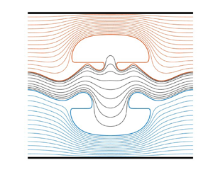There are now two symmetry-breaking bifurcation points ($F$ approximately 0.054 and 0.068) on the symmetric Boussinesq branch (blue) and two folded symmetry-breaking branches (red and yellow) grow from these points. Solutions (i) to (iv) in figure 5(c) are the almost symmetric solutions which can be seen both from their profiles and the fact that they lie near the symmetric branch of the Boussinesq approximation. On the other hand, solutions (v) to (viii) are almost limiting profiles of the symmetry-broken waves. It is interesting to note that these solutions show some characteristics of mode-1 waves, which is probably due to the mode-resonance mechanism described below. Like the mode-1 waves, we also expect the corresponding limiting waves to have closed bubbles attached to $120^{\circ }$ angles. Solutions (iv), (vii) and (viii) are the almost limiting waves of this type. However, there are other possible limiting waves as solutions (v) and (vi) suggest. Taking solution (v) for example, one can infer that the upper interface (red) becomes self-intersecting if the local peak ($x\approx \pm 0.8$) touches the mushroom's base. In this fashion, there will be two closed fluid bubbles (of the upper fluid) which are symmetric with respect to the vertical lines $x=0$. A further discussion on this new limiting configuration is beyond the scope of the current paper and shall not be addressed here.

Figure 5. Numerical solutions of mode-2 waves with $R_1=1.01$, $R_3=0.99$, $h_1=1$, $h_3=1$, $k=1.5$. (a) Speed–energy bifurcation branches of the Euler case. (b) Speed–energy bifurcation branches of the Boussinesq case. (c,d) Typical wave profiles of Euler case which are labelled in (a) and plotted in two spatial periods.

For longer periodic mode-2 waves ($k$ decreasing) the complexity of the bifurcation curves increases as there is the possibility of important resonances between the mode-2 waves and the mode-1 waves. Analogous to the well-known case of Wilton ripples in capillary–gravity surface waves (Wilton Reference Wilton1915), it is possible to find two wavenumbers $k_1$ and $k_2$ such that

(4.2)\begin{equation} c_{p1}(k_1)=c_{p2}(k_2), \quad mk_1=nk_2, \quad \text{$n>m$ are two positive integers,}\end{equation}

where $c_{p1}(k_1)$ is the phase speed of the mode-1 waves for $k=k_1$ and $c_{p2}(k_2)$ is the phase speed of the mode-2 waves for $k=k_2$. A similar mechanism has been pointed out by Chen & Forbes (Reference Chen and Forbes2008) who focused on the case $m=1$. These resonances can be seen from figure 6, where we plot the dispersion relation curves for $R_1 = 1.1$, $R_3 = 0.9$, $h_1 = 1$ and $h_3 = 1$. For simplicity, we shall use the term $(m,n)$ resonance to denote such conditions. Three examples corresponding to $(1,2)$, $(1,3)$ and $(1,10)$ are shown in figure 6 by the three dashed horizontal lines. There exist a countable number of resonant pairs since $n/m\rightarrow \infty$ when $k_2\rightarrow 0$. These resonant pairs imply that if one chooses the wavenumber to satisfy (4.2), then, linearly, a mode-1 component and a mode-2 component coexist. This has consequences in the nonlinear solution branches.

Figure 6. Dispersion relation curves with $R_1 = 1.1$, $R_3 = 0.9$, $h_1 = 1$ and $h_3 = 1$. The upper and lower curves correspond to the mode-1 and mode-2 waves. The horizontal dashed lines represent three possible resonant pairs $(k_1, k_2)$ for which $k_1/k_2=2,3,10$, respectively.

In figure 7, we display the special example corresponding to the $(1,2)$ resonance of figure 6. In figure 7(a), the blue curve is the speed–energy bifurcation branch of solutions with $k = 0.97651$ (which corresponds to one branch of Wilton ripple-like solution), and the black dashed curve is the speed–energy bifurcation mode-1 waves with $k=1.953$ for which the energy is calculated in two spatial periods. Solution (i), which is labelled by a black dot, is a small-amplitude linear wave, so we plot the corresponding upper interface (red) and lower interface (blue) in figure 7(b), respectively. In the bottom subpanel of figure 7(b), we plot $|\hat \theta ^-|$ versus $n$ in a $\log$-scale, where $\hat \theta ^-$ denotes the Fourier coefficient of the lower interfacial inclination $\theta ^-$, and $n$ is the order of the Fourier modes. It is clear that only the first two Fourier modes are significant while the rest are tiny enough to be neglected. Because of the existence of the resonant pair, the wave profile of (i) exhibits a mixture of the mode-1 and mode-2 waves. When the value of $F$ increases, the energy monotonically grows until the mode-2 wave bifurcation curve intersects the mode-1 wave bifurcation curve near $F=0.1787$. The final solution (ii) is a mode-1 wave and is shown in the inset in figure 7(a). In general, this mode resonance still exists when $k_1/k_2$ is a rational number rather than just an integer. In this case, we expect to see $n$ mode-1 wave components coexist with $m$ mode-2 waves, at least in the linear region. Figure 8 displays an example with parameters: $R_1 = 1.01$, $R_3 = 0.99$, $h_1 = 1$, $h_3 = 1$ and $k=0.2525$. According to the dispersion relation, the $(2,7)$ resonance is predicted when $k_1 \approx 1.7679$ and $k_2 \approx 0.5051$. Therefore, we choose the length of the computing domain to support two mode-2 waves with $k=0.5051$ or seven mode-1 wave with $k=1.7679$. Three typical solutions are labelled on the local energy–speed bifurcation curve in figure 8(a), their wave profiles are plotted in figure 8(b). As the figure clearly shows, solution (i) is almost a standard mode-2 wave having two spatial periods. Solution (ii) has already generated some mode-1 components and clearly lost the double periodicity. Solution (iii) almost becomes a mode-1 wave and develops seven quasiperiodic mode-1 waves.

Figure 7. (a) Speed–energy bifurcation curves with $R_1 = 1.1$, $R_3 = 0.9$, $h_1 = 1$, $h_3 = 1$, $k=0.97651$ (blue, mode-2), and $k=1.953$ (black, mode-1). The energy of the mode-1 waves are calculated in two spatial periods. The figure in the inset box shows the wave profile of solution (ii). (b) The top and middle subpanels are the upper and lower interfaces of solution (i) in (a). The bottom subpanel displays the absolute value of $\hat \theta ^-$ of solution (i) in a log-scale, where $\hat \theta ^-$ is the Fourier coefficient of the lower interfacial inclination angle $\theta ^-$, and $n$ is the order of the Fourier modes.

Figure 8. (a) Speed–energy bifurcation curves with $R_1 = 1.01$, $R_3 = 0.99$, $h_1 = 1$, $h_3 = 1$ and $k=0.2525$. (b) Three typical wave profiles corresponding to the labelled solutions in (a). The red and blue curves are the upper and lower interfaces.

In fact, due to the nonlinearity, the resonant condition (4.2) only needs to be satisfied approximately to support the resonance. In figure 9, we plot six speed–energy bifurcation branches of the mode-2 waves with $R_1 = 1.1$, $R_3 = 0.9$, $h_1 = 1$, $h_3 = 1$ and $k=1$. The black dashed lines are the speed–energy bifurcation curve of the mode-1 waves with $k=2$. The blue curve and part of the red curve are of the $(1,2)$ resonant type. The wave profiles of solutions (i) and (ii) are shown in the two insets. This clearly indicates that they become the mode-1 waves with wavenumber $k=2$. Nine almost limiting wave profiles are shown in figure 10. Note that the blue curve is not the only one which intersects the mode-1 bifurcation curve, the cyan branch also has an intersection at solution (x). The corresponding profile is a rather nonlinear mode-1 wave with an overhanging upper interface. This means that the mode-resonance exists not only in the weakly nonlinear region but also when solutions become highly nonlinear. Solutions (v) to (ix) are similar to those shown in figure 5. However, solutions (iii), (iv) and (xi) suggest the existence of a new limiting wave, but we shall not discuss it in the current paper.

Figure 9. Energy–speed bifurcation curves and two related wave profiles of the mode-2 solutions with $R_1 = 1.1$, $R_3 = 0.9$, $h_1 = 1$, $h_3 = 1$ and $k=1$. Associated (almost) limiting waves are labelled by black dots on curves. The black dashed line is the energy–speed bifurcation of the mode-1 solutions for the same values of $R_1, R_3, h_1, h_3$ and $k=2$ whose energy is calculated in two spatial periods. The two insets show the wave profiles corresponding to (i) and (ii).

Figure 10. Almost limiting wave profiles corresponding to the nine labelled solutions (iii) to (xi) in figure 9.

An important question is how the bifurcation structure and wave profiles change when the five related parameters $R_1$, $R_3$, $h_1$, $h_3$ and $k$ are gradually varied. In general, if we change the depth $h_1$ and $h_3$ but keep the other parameters fixed, the bifurcation structures and solutions are quantitatively similar. Wave profiles become spatially longer (shorter) if the depth is increased (decreased). On the other hand, if we gradually change the values of $R_1$ and $R_3$ away from the weak density stratification, but keep $(R_1-1)/(1-R_3)$ constant, i.e. the lower and the upper layer have the same density variation to the density of the middle layer, then one generally observe that the adjacent solution branches gradually get farther away from each other in the speed–energy bifurcation space. In figure 11, we display two numerical results with $h_1=h_3=1$, $k=1$, $R_1=1.3$, $R_3=0.7$ (figure 11a) and $R_1=1.5$, $R_3=0.5$ (figure 11b). For these two cases, the bifurcation structure is complex and the Boussinesq approximation is no longer valid since the density stratification is no longer weak. Comparing the bifurcations and the almost limiting wave profiles displayed in figure 12 with the numerical results shown in figures 9 and 10, it is noted that the number of bifurcation branches is decreased to four and some typical solutions in figure 10 vanish. In fact, this was also found in the two-layer interfacial waves that some bifurcation branches gradually shrink and ultimately disappear in the bifurcation space when the related parameters are varied (Guan et al. Reference Guan, Vanden-Broeck and Wang2021a). Note that the $(1,2)$ resonance exists when $k\approx 1.1$ for $R_1=1.3$, $R_3=0.7$ and when $k\approx 1.43$ for $R_1=1.5$, $R_3 = 0.5$. Therefore, we do not directly observe the mode-resonant phenomenon for these two cases since the wavenumbers that we choose is not very close to these critical wavenumbers. However, solutions (i), (ii) and (iii) still display some characteristics of resonance and can be thought of as the nonlinear evolution of mode resonance. The waves in figure 12 show that the possible limiting configurations are either a closed bubble attached to a $120^{\circ }$ angle, or two closed bubbles located symmetrically to the vertical line $x = 0$, or special mode-1 waves having larger wavenumber. It is interesting to note that the almost closed bubble on the upper interface could have both upward and downward orientations.

Figure 11. (a) Speed–energy bifurcation curves of the mode-2 waves with $R_1 = 1.3$, $R_3 = 0.7$, $h_1 = 1$, $h_3 = 1$ and $k=1$. (b) Speed–energy bifurcation curves of the mode-2 waves with $R_1 = 1.5$, $R_3 = 0.5$, $h_1 = 1$, $h_3 = 1$ and $k=1$. The black dashed curve is the bifurcation of the mode-1 waves with the same parameters except $k=2$. The corresponding energy is calculated in two spatial periods.

Figure 12. Almost limiting wave profiles corresponding to the labelled solutions (i) to (vii) in figure 11.

If we fix the values of $R_1$, $R_3$, $h_1$ and $h_3$, but gradually decrease $k$, then we obtain a family of long waves which converges to generalised solitary waves. In this process, the bifurcation structure becomes even more complex since there emerge a number of new resonant pairs. In figures 13–15, we exhibit the numerical solutions for $R_1=1.01$, $R_3 = 0.99$, $h_1 = 1$, $h_3=1$ and $k=0.096$. According to the linear theory, we can predict the critical values of $F$ at which the mode-resonance occurs:

(4.3)\begin{equation} F = c_{p1}(nk), \quad \text{$n$ is a positive integer}, \end{equation}

where $c_{p1}(k)$ is the phase velocity of the mode-1 waves with wavenumber $k$. In figure 13(a), five critical values of $F$ corresponding to $n = 9$ to $13$ are shown by the five vertical dashed lines. To show the existence of the resonant mode-1 component, we select four typical solutions in the region close to the predicted critical values of $F$, display their profiles, as well as the corresponding $|\hat \theta ^{\pm }|$ in a $\log$-scale, where $\hat \theta ^{\pm }$ are the Fourier coefficients of the inclination angles of the upper and lower interfaces. It is interesting to note that this prediction gives fairly good agreement with the numerical results. More importantly, it indicates that close to these critical values there are new bifurcation branches. Therefore, the bifurcation structure is like a comb. Every branch has a part that belongs to the almost symmetric branch, and the symmetry-breaking part becomes a tooth of the comb at some turning points close to the predicted critical values of $F$. The second part of the whole bifurcation is shown in figure 14 as well as the four predicted critical values of $F$ corresponding to $n = 5$ to $8$. As can been clearly seen, the positions of these turning points gradually differ from the predictions when waves become nonlinear, and the solutions gradually develop profiles of typical mode-2 generalised solitary wave type. The $|\hat \theta ^-|$ plot does not clearly show the resonant mode-1 component since more Fourier modes come into play.

Figure 13. (a) Speed–energy bifurcation curves for $R_1=1.01$, $R_3 = 0.99$, $h_1 = 50$, $h_3=50$ and $k=0.096$. The vertical dashed lines denote the predicted value of $F$ where the mode-2 waves are resonant with the mode-1 waves having waves number $nk$. The corresponding values of $n$ are shown close to the vertical lines. (b) Typical wave profiles and related absolute value of one of $\hat \theta ^{\pm }$ of the labelled solutions (i) to (iv) in (a), where $\hat \theta ^-$ and $\hat \theta ^+$ are the Fourier coefficients of the inclination angle of the lower and upper interface.

Figure 14. (a) Continuation of figure 13(a). (b) Typical wave profiles and related absolute value of $\hat \theta ^{-}$ of the labelled solutions (v) to (viii) in (a).

Figure 15. Six different (almost) limiting wave profiles with $R_1=1.01$, $R_3 = 0.99$, $h_1 = 50$, $h_3=50$ and $k=0.096$.

If we follow different comb-teeth bifurcation curves and let the energy increase, then the wave profiles could develop rather different limiting configurations. In figure 15, we show six typical highly nonlinear solutions following those branches shown in figures 13 and 14. From top to bottom, these solutions come from the $(1,12)$, $(1,10)$, $(1,9)$, $(1,8)$, $(1,7)$ resonance teeth, and the rightmost almost symmetric branch in figure 14(a), i.e. the lower magenta branch. It turns out solutions could become pure mode-1 waves as shown in figure 15(a), or the long mode-1 waves with a distorted midsection and periodic mode-1 tails shown in figure 15(b–d), or the long mode-2 waves with periodic mode-1 tails shown in figure 15(e,f).

Figure 16 shows bifurcation curves for $R_1 = 1.01, R_3 = 0.99, h_1 = h_3 = 0.1$ and $k=0.1$. Here, the middle-layer is deep relative to the upper and lower layer, and the wave is relatively long. The main central pules of the resonant mode-2 waves in this case are found to be concave (that is, the upper interface is of depression, and the lower is of elevation). Note that in this case, the branches are found to cross the linear long-wave speed of mode-1, which for these parameters is given by $F\approx 0.0316$. This feature was also observed for mode-2 solitary waves (Barros et al. Reference Barros, Choi and Milewski2020; Doak et al. Reference Doak, Barros and Milewski2022), and indeed when the magenta branch exits the linear spectrum, the resulting solutions are true mode-2 solitary waves with no resonances (solution B in the figure). Although linear waves do not exist for speeds $F>0.0316$, nonlinear mode-1 solitary and periodic waves do, and the other branches which exit the spectrum still have resonances with nonlinear mode-1 waves.

Figure 16. (a) Speed–energy bifurcations of mode-2 waves with $R_1 = 1.01, R_3 = 0.99, h_1 = h_3 = 0.1$ and $k=0.1$. The black dashed line represents the max phase speed of mode-1 waves. (b) Solutions A and B labelled in (a).

When $R_1-1\neq 1-R_3$, there exists a kind of ‘trapped waves’ solution as shown by the typical solutions in figure 17. The related parameters are $R_1=1.01$, $R_3 = 0.95$, $h_1 = 1$, $h_3=1$ and $k=1$. According to the dispersion relation, a $(1,7)$ resonance exists when $k \approx 0.98472$. This explains the profile in figure 17(a) where seven oscillations are generated on the top interface in one spatial period. Surprisingly, there appears only one single wave on the lower interface. These waves are very similar to those previously obtained by Lewis, Lake & Ko (Reference Lewis, Lake and Ko1974) and Chen & Forbes (Reference Chen and Forbes2008). When the amplitude of the lower interface gradually increases, it develops a bell-shaped profile and the oscillations on the upper interface gathered in the region above the trough of the lower interface. It is worth mentioning that similar solutions have been previously discovered in Liapidevskii & Gavrilov (Reference Liapidevskii and Gavrilov2018) experimentally and in Doak et al. (Reference Doak, Barros and Milewski2022) numerically. Figures 17(c) and 17(d) show that the waves could become even more nonlinear so that the upper interface develops an overhanging profile and tends to become self-intersecting. One or several closed bubbles are almost formed for solutions on different bifurcation branches. These overhanging structures are locally similar to those profiles shown before, except that the bubble size is greatly decreased. The lower interface also becomes steep and even overhanging. If the value of $R_3$ is further decreased to zero, then the three-layer model approaches an ‘air–water–water’ setting. In this case, there are even more tiny oscillations on the upper interface and a large amplitude internal wave on the lower interface, which is a rough approximation of the real ‘surface-internal waves’ oceanic scenario.

Figure 17. Four typical wave profiles with $R_1=1.01$, $R_3 = 0.95$, $h_1 = 1$, $h_3=1$ and $k=1$.