


1. Introduction
Formal risk analysis may be considered the best method for evaluating the danger people face from avalanches, and for introducing proper land-use regulation in endangered areas. Estimating avalanche risk gives the information in a manner that is easy to understand and interpret, and enables a comparison to be made with other types of naturally or artificially induced risk. Nevertheless, only recently have such approaches emerged for analyzing the effect of snow avalanches (Reference WilhelmWilhelm, 1998; Reference Jónasson, Sigurðsson and ArnaldsJónasson and others, 1999; Key-lock and others, 1999; Keylock and Reference Barbolini and SaviBarbolini, 2001), and, except for Iceland (Reference Jóhannesson and ArnaldsJóhannesson and Arnalds, 2001), none of the existing zoning techniques adopts the risk approach explicitly.
According to the Committee on Risk Assessment of the Working Group on Landslides of the International Union of Geological Sciences (IUGS, 1997), quantitative risk analysis involves expressing the risk as a function of the hazard, the elements at risk and the vulnerability, where these terms are defined inTable 1 according to the IUGS (1997) guidelines.
Table 1. Definitions of risk terminology following appendix 1 of IUGS (1997). The word “avalanche” has been substituted for “landslide”

Before the risk can be measured, one must decide what unit to use. There are several possible definitions of this unit. One might measure the risk as the yearly expected value of property loss due to avalanches (economic risk, measured for instance in €/year; see Reference WilhelmWilhelm, 1998), or as the number of people expected to be killed annually by avalanches in the area concerned (measured in deaths/year; see Wilhelm, 1998). In the present study, in accordance with the proposal of Reference Jónasson, Sigurðsson and ArnaldsJónasson and others (1999), we measure the risk as the annual probability of being killed by an avalanche if one lives or works in a building under a hazardous hillside (individual risk). Therefore human life is considered to be the element at risk (according to Table 1). To make this definition workable, one must also specify the proportion of time spent inside the building. As a reference value, we calculate the individual risk based on the assumption that the person is present in the building 100% of the time, and refer to this as local risk. This is the same unit as the one chosen by Reference Jónasson, Sigurðsson and ArnaldsJónasson and others (1999) for avalanche risk mapping and by Reference Evans, Foot, Mason, Parker and SlaterEvans and others (1997) for aeroplane crash risk. The actual risk for a person is only a fraction of the local risk, depending on the fraction of time he/she spends in the building (usually referred to as the exposure), which in turn depends on the age of the person and on the type of building (e.g. for children or old people at home, the exposure might be as high as 75%, compared with about 30% for people at their place of work). If a typical degree of exposure is defined for different types of buildings (dwellings, commercial buildings, cottages, etc.), as well as an acceptable risk level, local risk can be used as a feasible base for regulating land use in avalanche-prone areas, as suggested by the current Icelandic legislation (Reference Jóhannesson and ArnaldsJóhannesson and Arnalds, 2001).
Within such an approach the vulnerability (according to Table 1) becomes the probability of death for a person inside a house hit by an avalanche. This probability, in the following indicated as d, depends on the type of building and on the avalanche dynamic characteristics. In the present study, vulnerability is defined assuming a given structure type and as a function of avalanche velocity. Accordingly, the fatality ratio should broadly correlate with the impact pressure with which the avalanche strikes the building, and, therefore, ultimately with the avalanche velocity. Many authors (Reference MellorMellor, 1978; Reference McClung and SchaererMcClung and Schaerer, 1993; Keylock and Reference Barbolini and SaviBarbolini, 2001), at least for flowing avalanches hitting large obstacles (such as buildings), have proposed a relation between avalanche velocity (υ) and impact pressure (pimp:) of the type:
where ρ is the avalanche density. Equation (1) is also suggested for engineering design by the Swiss and Russian Guidelines (Reference Salm, Burkard and GublerSalm and others, 1990; Bozhinskiy and Losev, 1998), and has been adopted in the present study with ρ set to 300 kgm–3. Undoubtedly, lack of knowledge of how avalanche impact damages structures and causes fatalities is a major limitation on any current avalanche risk assessment. Therefore, the effect of using different vulnerability relations on the resulting risk mapping will be explored.
The hazard component of risk (Table 1) is the main focus of this study. So far, this component has been derived by statistical methods, fitting a statistical distribution to historical avalanche events of known runout distances in a given avalanche path. Because of the usual lack of a sufficient number of recorded events, some authors tried to circumvent the problem by standardizing records from several different avalanche paths to produce a combined artificial history for an average avalanche path within a mountain region. Avalanche events have been transferred between paths either by topographical criteria (Reference Keylock, McClung and MagnússonKeylock and others, 1999) or by using physical models (Reference Jónasson, Sigurðsson and ArnaldsJónasson and others, 1999). However, the main problem with statistical approaches remains to be solved, which is to extrapolate the empirical probability distribution fitted to field data in order to estimate the avalanche frequency in areas not covered by historical information.
In this paper, we introduce a new methodology to estimate the hazard component of avalanche risk. The probability Px, y(v) that a given velocity (υ) will be reached or exceeded at any given point (x, y) of the avalanche path is determined by:

where f (V) is the probability density function (PDF) of the avalanche release volume V, and ![]() is the probability that the avalanche velocity will exceed υ at the location (x, y) if the avalanche release volume is V. This latter probability is calculated by avalanche dynamics simulations. Risk at a given location (x, y) is then calculated as:
is the probability that the avalanche velocity will exceed υ at the location (x, y) if the avalanche release volume is V. This latter probability is calculated by avalanche dynamics simulations. Risk at a given location (x, y) is then calculated as:

where d(υ) is the vulnerability relation and px, y(υ) is the PDF of avalanche velocity at the location (x, y), obtained by derivation from ![]() with Px, y(υ) defined in Equation (2). The specific methods introduced to determine the function Px, y(υ) and d(υ) are described in sections 2 and 3, respectively. In section 4 an application of the procedure to a real-world mapping problem is presented. The potential of the proposed approach for evaluating the residual risk after the implementation of defensive structural work is also shown.
with Px, y(υ) defined in Equation (2). The specific methods introduced to determine the function Px, y(υ) and d(υ) are described in sections 2 and 3, respectively. In section 4 an application of the procedure to a real-world mapping problem is presented. The potential of the proposed approach for evaluating the residual risk after the implementation of defensive structural work is also shown.
2. The Hazard Component of Risk, Px , y(υ)
The probability that a given point along a slope will be reached by an avalanche with a velocity equal to or higher than a fixed value υ can be evaluated in principle by considering the release probability of a snow volume V and the probability that the given point along the avalanche path will be reached by an avalanche with a velocity not lower than υ, given the avalanche release volume is V. If the avalanche dynamics is simulated by means of a one-dimensional mathematical model, the computational domain can be represented in a Cartesian plot (x, z), where x is the progressive distance from the fracture line and z is the elevation. In this way, each point on the slope can be identified by means of the x coordinate (so that in Equations (2) and (3) the pair x, y reduces to the coordinate x alone). Within this simplified one-dimensional scheme, the avalanche-release conditions reduce to slab length and fracture depth. Assuming for the slab length a deterministic pattern dependent on the release zone topography and not related to the avalanche frequency at all, the release volume V in Equation (2) will only depend on the release depth h.
Introducing a random variable H such that:

the probability P that the point x in the runout zone will be reached by an avalanche with a velocity ≥υ (H = 1) can be expressed as:

where f(h) is the PDF of the release depth h and ![]() is the probability that at point x the avalanche velocity will exceed υ given a release depth equal to h. Equation (4) is based upon composed and total probability axioms, under the assumption that
is the probability that at point x the avalanche velocity will exceed υ given a release depth equal to h. Equation (4) is based upon composed and total probability axioms, under the assumption that ![]() and f(h) are unrelated. A similar definition has been proposed by the U.S. Federal Emergency Management Agency (FEMA, 1990) for mapping areas affected by debris flows.
and f(h) are unrelated. A similar definition has been proposed by the U.S. Federal Emergency Management Agency (FEMA, 1990) for mapping areas affected by debris flows.
The function f(h) is estimated by statistical inference from snowfall data records (see section 2.1), whereas the probability ![]() is determined by avalanche dynamics modelling (see section 2.2). Because the avalanche dynamic behaviour must be explored over a wide range of release depths (Equation (4)), the dependence of the model parameters on the avalanche size is crucial (see section 2.3).
is determined by avalanche dynamics modelling (see section 2.2). Because the avalanche dynamic behaviour must be explored over a wide range of release depths (Equation (4)), the dependence of the model parameters on the avalanche size is crucial (see section 2.3).
2.1. Estimation of the release-depth PDF, f (h)
According to Reference Salm, Burkard and GublerSalm and others (1990) and Reference Burkard and SalmBurkard and Salm (1992), the release or fracture depth h can be expressed as a function of the 3 day increase in snow depth ΔH(3d), the additional snowdrift depth ΔHsd and the average inclination of the release zone θ as follows:
where s(θ) is a slope factor which takes into account that the release depth decreases with increasing slope angle (Reference Salm, Burkard and GublerSalm and others, 1990). Assuming that ΔHsd can be characterized by an estimated average value (Reference Salm, Burkard and GublerSalm and others, 1990), ΔH(3d) is the only random variable in Equation (5). Given the linear relationship between h and ΔH(3d), the following relation holds between their PDFs:

The PDF of ΔH(3d); fΔH(3d), can simply be inferred by statistical analysis, i.e. by fitting a representative sample of maximum annual values of ΔH(3d) with a theoretical distribution function that shows a good adaptation to the data. Due to the usual lack of snowfall data and to the spatial randomness of ΔH(3d) – meteorological gauging stations are mostly located at lower altitude than the release zones − “regional analysis” techniques (Reference KiteKite, 1988; Cunnane, 1989) provide an effective way of more accurately estimating the PDF of ΔH(3d) (Reference Barbolini, Natale and SaviBarbolini and others, 2002), and have been used in the present study.
2.2. Estimation of the probability 
To simulate the avalanche propagation and to evaluate the probability ![]() VARA1D, the one-dimensional version of the VARA avalanche dynamics models (Reference Natale, Nettuno and SaviNatale and others, 1994; Reference BarboliniBarbolini, 1998; Reference Barbolini, Gruber, Keyloch, Naaim and SaviBarbolini and others, 2000; Reference Barbolini and SaviBarbolini and Savi, 2001), has been used. Given that the avalanche release depth is h, the avalanche dynamics is simulated with the VARA1D model:
VARA1D, the one-dimensional version of the VARA avalanche dynamics models (Reference Natale, Nettuno and SaviNatale and others, 1994; Reference BarboliniBarbolini, 1998; Reference Barbolini, Gruber, Keyloch, Naaim and SaviBarbolini and others, 2000; Reference Barbolini and SaviBarbolini and Savi, 2001), has been used. Given that the avalanche release depth is h, the avalanche dynamics is simulated with the VARA1D model: ![]() is set to 1 if the avalanche reaches point x with a velocity>υ; otherwise it is set to zero.
is set to 1 if the avalanche reaches point x with a velocity>υ; otherwise it is set to zero.
2.3. Dynamic model calibration
The VARA1D model has been calibrated reproducing historical events from three different Italian alpine ranges: Val di Rabbi (Province of Trento), Val Brembana (Province of Bergamo) and Valtellina (Province of Sondrio). Validation data included the longitudinal profile of the path, the upper and lower limits of the release area, the fracture depth, the runout distance and sometimes some rough information about the deposition height. We calibrated the model by identifying the values of the friction parameters μ and ξ that minimize the differences between computed and observed runout distance. Further information is required to avoid over-parameterization of the model, since the same runout distance can be obtained using different combinations of the values of μ and ξ. If some information on the spatial distribution of the avalanche deposits was known, the values of the parameters were estimated by minimizing the mean square error between observed and computed runout distance and maximum deposition height. If no information other than the runout distance was available, we reduced the range of admissible values of μ and ξ by imposing limits on the maximum avalanche velocity, according to measurements from Roger’s Pass, British Columbia, Canada by Reference McClung and SchaererMcClung and Schaerer (1993, fig. 5.32).
We found a significant decrease in μ as the avalanche frequency decreases (and as the release depth h increases); this trend is also suggested in the Swiss Guidelines (Reference Salm, Burkard and GublerSalm and others, 1990). However, it seems reasonable to introduce a relationship between μ and h of the type μ= F(h) only for a specific avalanche site, since the same release depth can be either extreme or very frequent for two different sites. For this reason, the values of μ and hmust be scaled by considering average site-specific values, and a relationship of the type μ/μ0 = F(h/h0) must be searched. On the basis of the model calibration, we identified a set of pairs μi;j and hi;j (j=1, . . ., M and i=1, . . ., Nj with M the number of sites and Nj the number of the calibration events available for the jth site). These values are scaled for each site with the respective average value of μ(μ0j) and mean annual release depth (h0j), to obtain the set of pairs (μi;j/μ0j; hi;j/h0j), which are plotted in Figure 1. The dimensionless value of the friction coefficient μ was found to be significantly related to the dimensionless release depth (the t test for the coefficient of correlation, R= 0.79, is verified with P =0.01). A least-squares regression gives:

Fig. 1. Normalized friction coefficient μ/μ0 υs normalized release depth h/h0 for 39 calibration events in 17 avalanche paths. The regression line (Equation (7)) has R = 0.79 and σ = 0.095, with R coefficient of correlation and σ standard error of estimate.

For a given avalanche site, once the values of μ0 and h0 have been estimated, Equation (7) gives the site-specific relation between μ and h, which, in turn, once a typical release area is defined, allows the site-specific relationship between μ and the release volume V to be defined.
3. The Vulnerability Component of Risk, d(v)
Reference Jónasson, Sigurðsson and ArnaldsJónasson and others (1999) linked avalanche speed to survival probability inside a building by a maximum likelihood technique. Their analysis was based on data from the 1995 Icelandic avalanches at Súdavik and Flateyri, which damaged a total of 32 houses where 93 people were staying, causing 34 fatalities. They obtained the following vulnerability relation d(υ), indicating the probability of death inside a house as a function of the avalanche velocity:

where k = 0.00130, c = 0.05, a = 1.151, b =18.61 and υ1 = 23ms–1 (Fig. 2). The vulnerability decreases progressively to zero with decreasing avalanche velocity; there is an upper limit of 0.95 if the avalanche velocity becomes indefinitely high. It is therefore implicitly assumed that a loss of life is always possible with a non-zero velocity and that, regardless of how fast the avalanche travels, some people will always survive.
Fig. 2. Vulnerability vs avalanche velocity. The dashed bold line shows the relation proposed by Reference Jónasson, Sigurðsson and ArnaldsJónasson and others (1999) (Equation (8)); the solid bold line shows the relation including velocity thresholds derived in this study based on Icelandic data (Equation (9)). The other two curves represent the vulnerability relations for (Icelandic) reinforced structure for the case with (solid) and without (dashed) thresholds.
However, it seems reasonable to assume that people are safe inside a building for low-intensity events. Therefore it is proposed to introduce a lower threshold for the velocity, υlt, below which vulnerability can be set to zero. This is in accordance with the proposal of Reference Keylock, McClung and MagnússonKeylock and others (1999) who indicate zero vulnerability for the smallest avalanche size (1 and 2 according to the Canadian Avalanche Size Classification, with typical impact pressure in the range 1–10 kPa; see Reference Keylock, McClung and MagnússonKeylock and others, 1999, tables 1 and 9). Keylock and Reference Barbolini and SaviBarbolini (2001) presented a vulnerability relation which also contains an upper threshold for the velocity, υut, which was estimated to be about 15 ms–1 for Icelandic types of building. For velocity values higher than υut the vulnerability was set to 1. The existence of such a threshold is more questionable, given that even the complete destruction of a building does not necessarily entail the death of a person staying inside. Reference WilhelmWilhelm (1998) presented plots of the susceptibility to damage (S) as a function of impact pressure for different types of construction (S varies between 0 (no damage) and 1 (house destruction)). All these curves showed a destruction limit (varying between 10 and 50 kPa depending on the construction type). However, a probability of death 51 for people inside a destroyed house was suggested. A similar result can be derived from the vulnerability data presented in Reference Keylock, McClung and MagnússonKeylock and others (1999).
In order to explore the effect on the risk mapping of introducing thresholds in the vulnerability relation, we have reworked the Icelandic data (Reference Jónasson, Sigurðsson and ArnaldsJónasson and others, 1999, table 7), to obtain a vulnerability relation with thresholds. This curve, derived by fitting a second-order polynomial to the data of Table 2, is presented in Figure 2 and has the following form:
Table 2. Dependence of death rate d on avalanche velocities v with respect to the 1995 avalanche events in Súdavik and Flateyri, Iceland
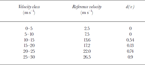

The lower velocity threshold is 3.5 ms–1, corresponding to an impact pressure of about 3 kPa according to Equation (1). This seems to be a reasonable value, given that Reference WilhelmWilhelm (1998) suggests a value of about 2.5 kPa as the building damage threshold for the lowest quality of construction (“light construction”). The upper velocity threshold gives an impact pressure of about 250 kPa (see Equation (1)), a value about an order of magnitude higher than the impact pressure that Reference McClung and SchaererMcClung and Schaerer (1993) indicate can destroy a wood frame house (30 kPa). This partly justifies our first estimate of the threshold for 100% fatalities within an unreinforced structure with poorly supported walls, as is the case for Icelandic houses.
Both vulnerability relations (Equations (8) and (9)) are derived from Icelandic data. It should be pointed out that most of the houses in the avalanche hazard zones of Iceland are fairly weak, made of timber or unreinforced concrete, with relatively large windows facing the mountain slope. Typical buildings in Alpine villages are suggested to be less vulnerable, and using Equation (8) or (9) might overestimate the actual risk levels. Using earthquake data, Reference Keylock, McClung and MagnússonKeylock and others (1999) suggested that for reinforced concrete structures vulnerability values can be assumed to be about 60% of those for low-quality buildings. Applying this ratio to our case, the residual vulnerability in Equation (8) decreases from 0.95 to 0.57, whereas the upper and lower velocity thresholds remain unchanged in Equation (9). In fact, reinforcing a structure should lead to an increase of both υut and υlt. Nevertheless, the residual vulnerability associated with a random chance of survival independent of avalanche intensity should not be influenced by structural reinforcement. Re-analyzing the data presented by Reference Keylock, McClung and MagnússonKeylock and others (1999), we have obtained an average rate of velocity increase of about 1.37 which leads, after reinforcement, to the same vulnerability value as before. Using this value to correct Equations (8) and (9), we have obtained the vulnerability relations for (Icelandic) reinforced structures, presented in Figure 2 for the case without and with thresholds, respectively. We may tentatively assume the vulnerability of Alpine buildings lies between the reinforced and non-reinforced Icelandic cases.
4. Case Study
4.1. Description of the site
The methodology previously described is applied to the Val Nigolaia avalanche site, a path located in the Italian Alps, within the Autonomous Province of Trento. Val Nigolaia is a tributary valley of Val di Rabbi that originates from the Castel Pagano top crest, at about 2600ma.s.l. The site is mainly channelled and covers a vertical drop of about 1500m (Fig. 3); its length is about 3 km. The release area, with a south-southwest aspect, is situated at approximately 2550–2200ma.s.l. and covers an area of about 0.095 km2, with an inclination of 35–45°. The track is constituted by a very narrow channel (about 10–15m wide); its slope gradually decreases from about 30° in the upper part to about 20° in the lower part. The track terminates at about 1250ma.s.l., where the deposition zone begins, represented by a fairly large alluvial fan. In the deposition zone, the slope gradually decreases from 15° in the upper part of the fan to a nearly flat zone close to the Rabbies river. The biggest known event on this path occurred in 1931: a huge wet-snow avalanche affected the western part of S. Bernardo village, damaging some buildings and depositing snow masses down to the Rabbies river (Fig. 3).
Fig. 3. Map of the avalanche site Val Nigolaia. The runout area, indicated by the rectangle, is shown in Figure 7.
4.2. Application of the methodology
In the simulations, the release length L is held constant and set to L = 500 m.The upper limit of the release area is fixed at 2550ma.s.l., according to chronicle information. The friction coefficient ξ is set to 5900 ms–2 (the mean of the calibrated values over the Val Nigolaia site) and kept constant in all the simulations, in accordance with the Swiss Guidelines (Reference Salm, Burkard and GublerSalm and others, 1990) which suggest that this parameter is mainly influenced by the degree of canalization and roughness of the track and not by the avalanche size. The average calibration value of the friction coefficient ξ may seem to be surprisingly high if compared to the reference values proposed in the Swiss Guidelines (Reference Salm, Burkard and GublerSalm and others, 1990), but this relates to a general tendency of “hydraulic-type” dynamic models to require larger values of ξ than “centre-of-mass-type”dynamic models (Reference Barbolini, Gruber, Keyloch, Naaim and SaviBarbolini and others, 2000). The friction coefficient μ is varied with the fracture depth according to Equation (7).
Px(υ) for any given position x of the runout areawas estimated for 60 different velocities, from 0.5 to 30 ms–1 with an increment step of 0.5 ms–1. Velocities higher than 30 ms- 1 are never obtained below 1250ma.s.l., where risk calculations are of interest. A position x and a velocity threshold υ having been fixed, Px(υ) is estimated by numerical integration of Equation (4), which reads:

and requires the following steps: a value of the fracture depth hi is assigned; the value of f(hi) is evaluated from the PDF of h, shown in Figure 4 for the site under analysis; the value of μi is computed by means of Equation (7), adopting h0 = 0.5 m and μ0 = 0.26 (estimated average values of the release depth h and of the friction coefficient μ for the site under analysis); the propagation of the ith avalanche is simulated by means of the VARA1D code; if the considered point (x) of the computational grid is reached by the avalanche with a velocity greater than υms–1, then ![]() otherwise
otherwise ![]() The above steps are repeated 40 times for each considered velocity threshold (we varied h from 0.1m to 2 m, with an increment of 0.05m), the values of the summation terms in Equation (10) are evaluated, and the probability Px(υ) can be calculated for the selected values of velocity. A typical result of this computation is shown in
The above steps are repeated 40 times for each considered velocity threshold (we varied h from 0.1m to 2 m, with an increment of 0.05m), the values of the summation terms in Equation (10) are evaluated, and the probability Px(υ) can be calculated for the selected values of velocity. A typical result of this computation is shown in ![]() . px(υ) is obtained by numerical derivation of (see Fig. 5). Of course, both Px(υ) and px(υ) change as the position x along the path changes.
. px(υ) is obtained by numerical derivation of (see Fig. 5). Of course, both Px(υ) and px(υ) change as the position x along the path changes.
Fig. 4. PDFof the release depth h for the Val Nigolaia path, obtained by “regional analysis” of annual maximum of the snow-depth increase over 3 days, ΔH(3d) (eight gauging stations for a total of 158 annual maxima). The regional data have been fitted to a generalized extreme values (GEV) distribution, with parameters estimated using the average-weighted-moments technique.
Fig. 5. Probability that the avalanche velocity exceeds υ at the location x, Px(υ) (solid line), and PDF of the avalanche velocity υ at the location x, px(υ) (dotted line), relative to the position along the slope given by x = 2200 m, corresponding to an altitude of 1220 m a.s.l. (the fan apex, approximately).
To obtain risk, Equation (3) is solved numerically:

To solve Equation (11) for any given location x, it is necessary to fix a velocity value υi; to estimate px(υi) from the PDF px(υ) relative to the selected location (see Fig. 5 for the location x = 2200m); and to estimate d(υi) from the chosen vulnerability relation. The previous steps are repeated 60 times, varying υ from 0.5 to 30ms–1, with an increment step of 0.5ms–1. The risk was estimated using the different vulnerability relations presented in Figure 2. Risk was also estimated assuming that part of the release zone is protected by snow bridges (about 40% of the potential release area, from 2550 to 2350ma.s.l.; see Fig.3). In this latter case, the release scenarios and the friction parameters were adjusted accordingly.
4.3. Results
Results of the simulations are summarized in Table 3. Using the vulnerability relation given by Reference Jónasson, Sigurðsson and ArnaldsJónasson and others (1999) (Equation (8)), we obtain risk values ranging from about 10–1 to 1.4×10⁻⁴ going from the upper part (fan apex, z = 1200ma.s.l.) to the lower part (river location, z = 1090ma.s.l.) of the runout area. Use of a vulnerability relation that includes thresholds (Equation (9)) leads to smaller risk values in the lower part of the runout zone (in particular in the area below the provincial road, i.e. for z < 1110ma.s.l.), with maximum differences up to 60% (Fig. 6). In fact, introducing a lower velocity threshold in the vulnerability relation reduces the risk level at smaller velocities, i.e. in the terminal part of the deposition zone. For the considered case, 3×10⁻⁴ and 1×10⁻⁴ risk lines are moved up-slope by about 10 and 25 m, respectively.
Fig. 6. Difference between risk estimates based on vulnerability Equation (8), taken from Reference Jónasson, Sigurðsson and ArnaldsJónasson and others (1999), and Equation (9), derived in this study based on Icelandic data and including upper and lower velocity thresholds, as a function of location along the path (expressed in m a.s.l.).
Table 3. Risk calculation in the runout area for different modelling assumptions

Use of the vulnerability relation for reinforced structures, of course, leads to lower risk values throughout the runout area (see Table 3). Differences with respect to the non-reinforced building case are of the order of about 45% for all the locations in the deposition zone. Assuming a relevant part of the release area is protected with retaining structures (see Fig. 3) leads to considerably reduced risk values in the runout area (Table 3). In particular, the risk approaches zero below 1100ma.s.l.
In Figure 7, the positions of the calculated risk levels 3610–4 and 0.3610–4 are indicated for three different modelling assumptions. These two risk levels are relevant for hazard mapping according to the Icelandic regulation (Reference Jóhannesson and ArnaldsJóhannesson and Arnalds, 2001). In particular, a calculated risk below 0.3610–4 is considered acceptable for any kind of land use, whereas major restrictions on land use are applied if the risk is 43610–4. For the site under analysis, the risk levels appear to be unacceptably high in the inhabited areas located at the valley bottom (Fig. 7), even if the average value lies between the reinforced and non-reinforced Icelandic cases, which seems a reasonable assumption for Alpine buildings. The protection of part of the release area with retaining structures considerably improves the safety of the population living in the endangered areas, and acceptable risk levels are attained over most of S. Bernardo village.
Fig. 7. Risk mapping according to different modelling assumptions.
5. Concluding Remarks
A new method for estimating risk in avalanche-prone areas has been proposed. Risk is defined as the yearly probability of being killed by an avalanche if one lives or works permanently in a building under a hazardous slope. Vulnerability, expressing the probability of death, is given as a function of the velocity of the avalanche hitting the building, according to previous formulations. The main innovation with respect to the current approaches is the use of an avalanche-dynamics model to estimate the hazard component of risk, i.e. the probability of having a given velocity for any fixed location along the avalanche path. So far the methodology has been implemented in a one-dimensional framework. However, extension to two dimensions is in principle quite straightforward, and simply requires the use of a two-dimensional dynamic model. The use of dynamic models has the twofold advantage of: (i) avoiding the problem of statistical inference from runout data, which in principle is inappropriate for extrapolations to undocumented areas; and (ii) estimating systematically the residual risk after the implementation of defence works. Accordingly, the method could provide a sound base for cost–benefit evaluations.
A relevant limit of our procedure is the lack of knowledge of vulnerability, i.e. how avalanche impact damages structures and causes fatalities. A fatality ratio which is a function of the avalanche velocity alone, such as the one we have used, is of course an oversimplification. More complex formulations that consider other dynamical parameters than velocity (e.g. the flow depth) will improve the method significantly. Furthermore, so far we have used relations based on Icelandic data. Specific studies are needed to define vulnerability relations more suitable for typical Alpine buildings. The possible existence of velocity thresholds in the vulnerability relation, as well as their effect on risk mapping, is another point that requires further investigation.
The uncertainties affecting the application of the dynamic model (related to either release conditions or friction-parameters estimate), as well as those underlying the definition of the vulnerability relation, can easily be incorporated into the methodology by using Monte Carlo simulation techniques, according to recent proposals (Reference Barbolini and SaviBarbolini and Savi, 2001; Reference Barbolini, Natale and SaviBarbolini and others, 2002). This point will be addressed as the most immediate follow-up to this work.
Acknowledgement
This research has been financially supported by the National Group for the Prevention of Hydrogeological Disasters (GNDCI) of the National Research Council of Italy (CNR). The authors wish to gratefully acknowledge L. Natale for his guidance in the development of this work, and G. Tecilla, M. Gaddo and G. Fruet from the Avalanche Office of the Autonomous Province of Trento for supporting the data collection.


