


1. Introduction
Transition from stability to instability in fluid flows is a subject widely explored in the literature. Bénard (Reference Bénard1901) was among the first to study it experimentally when he observed the appearance of convection cells in a thin layer of fluid after heating it from below beyond a certain critical temperature difference. The first explanation for this phenomenon was proposed by Rayleigh (Reference Rayleigh1916), who used a linear stability analysis to introduce buoyancy as the driving mechanism, which is the reason why this became known as the Rayleigh–Bénard problem. Many decades later, however, Pearson (Reference Pearson1958) also used linear stability analysis to propose a second explanation. He pointed out that the small film thickness employed by Lord Rayleigh essentially renders buoyancy effects negligible and, in turn, promotes surface tension gradients as the driving mechanism. The natural convection described by the Rayleigh–Bénard problem also occurs in a fluid saturated porous medium, in which case it is known as the Darcy–Bénard problem. Horton & Rogers (Reference Horton and Rogers1945) as well as Lapwood (Reference Lapwood1948) were the first to investigate its linear instability. Prats (Reference Prats1966) was the first to extend it to include a horizontal throughflow and, hence, to consider mixed convection.
The above-mentioned studies focus on the asymptotic behaviour of individual normal modes in either time or space. This eigenvalue, or modal, based description is the traditional way linear stability analyses have been performed (Chandrasekhar Reference Chandrasekhar1961; Drazin & Reid Reference Drazin and Reid1981). Some key developments, however, have appeared since then. When the disturbance is local, i.e. it does not vary in the direction of the longitudinal flow, at least in an approximate sense, convective and absolute instability concepts took over the previous temporal/spatial understanding (Huerre & Monkewitz Reference Huerre and Monkewitz1990). When the disturbance is no longer local, parabolised stability (Herbert Reference Herbert1997) and global stability (Theofilis Reference Theofilis2011) concepts can be employed. Adjoint equations (Luchini & Bottaro Reference Luchini and Bottaro2014) also deserve special mention, since they have been connected to absolute instability in both discrete (Lesshafft & Marquet Reference Lesshafft and Marquet2010) and continuous (Alves et al. Reference Alves, Hirata, Schuabb and Barletta2019) senses. Many of these techniques have been applied to both natural and mixed convection in porous media. Most cases focus on convective instabilities (Nield & Bejan Reference Nield and Bejan2006), but there have been some recent attempts to investigate absolute instabilities as well (Barletta Reference Barletta2019; Barletta, Celli & Alves Reference Barletta, Celli and Alves2020; Schuabb, Alves & Hirata Reference Schuabb, Alves and Hirata2020).
On the other hand, the short time/space behaviour of superposed normal modes can also be relevant. This non-modal description is key in explaining transition in modally stable flows under subcritical conditions (Schmid Reference Schmid2007). In general, Rayleigh–Bénard-type problems are self-adjoint and non-modal growth is not possible. This can change, however, in the presence of throughflow. Biau & Bottaro (Reference Biau and Bottaro2004) studied the effect of stable thermal stratification in shear flows whereas Sameen & Govindarajan (Reference Sameen and Govindarajan2007) studied the effect of wall heating in channel flows from the perspective of both modal and non-modal linear growth. Finally, Jerome, Chomaz & Huerre (Reference Jerome, Chomaz and Huerre2012) studied non-modal growth in both Rayleigh–Bénard–Poiseuille and Rayleigh–Bénard–Couette problems. In the context of porous media flows, only a few studies have dealt with the non-modal linear growth of disturbances, but they focused on density-driven instability (Rapaka et al. Reference Rapaka, Chen, Pawar, Stauffer and Zhang2008, Reference Rapaka, Pawar, Stauffer, Zhang and Chen2009).
One of the main goals of the present paper is to fill this gap, investigating modal as well as non-modal mechanisms for linear disturbance temporal growth that might exist for flows in porous media. Another goal is to do so while also considering the influence of viscous dissipation effects, often neglected due to their small magnitude. Gebhart (Reference Gebhart1962) has identified, however, the parametric conditions under which viscous dissipation can be relevant for natural convection in pure fluids. Furthermore, mixed convection renders viscous dissipation effects even more important due to the added forced component. In the context of porous media, the former was shown to be true by Nakayama & Pop (Reference Nakayama and Pop1989), where Murthy (Reference Murthy1998) extended this study to show that this is also true for the latter. According to Gebhart (Reference Gebhart1962), viscous dissipation effects can be dominant in many scenarios. He mentioned processes under a strong gravitational field (e.g. on larger planets), devices operating at high rotative speeds (e.g. internal cooling of turbine blades) as well as processes with large characteristic lengths (e.g. geophysical flows). Nield (Reference Nield2000) included particle bed nuclear reactors among possible interesting applications. Furthermore, Magyari, Rees & Keller (Reference Magyari, Rees and Keller2005) pointed out that many natural convection processes could be qualitatively altered by viscous dissipation effects even when they appear negligible. The characteristic dimensionless parameter quantifying the strength of the viscous dissipation effect for buoyant flows is today known as Gebhart number,  $Ge$, which can be interpreted as the ratio between the kinetic energy of the flow and the heat transferred to the fluid (Gebhart Reference Gebhart1962). Gebhart (Reference Gebhart1962) and, after him, Turcotte et al. (Reference Turcotte, Hsui, Torrance and Schubert1974) were the first to propose it, although they did so using a different name, i.e. the dissipation number. Nevertheless, they showed that such a parameter is usually small, but can achieve order unity under the aforementioned scenarios.
The effect of viscous dissipation on the onset of instability for several mixed convection problems in porous media was investigated in a series of studies. Barletta, Celli & Rees (Reference Barletta, Celli and Rees2009a) and Storesletten & Barletta (Reference Storesletten and Barletta2009) were the first to study the particular case where the internal heating generated by viscous dissipation is the sole cause of destabilisation. In their studies, no additional thermal forcing was imposed either internally or externally, namely through the walls or otherwise. The combined effect of internal heating through viscous dissipation and external heating through different thermal boundary conditions was studied by Barletta & Storesletten (Reference Barletta and Storesletten2010) as well as Barletta, Celli & Nield (Reference Barletta, Celli and Nield2010) and Nield, Barletta & Celli (Reference Nield, Barletta and Celli2011). Nield & Barletta (Reference Nield and Barletta2010) also explored two different models for the viscous dissipation effect. Viscous dissipation effects on non-Darcy models for flows in porous media were explored by Barletta, Celli & Rees (Reference Barletta, Celli and Rees2009b) and Barletta, di Schio & Celli (Reference Barletta, di Schio and Celli2011b) whereas thermal non-equilibrium, heterogeneity and viscoelastic fluid models were explored by Barletta & Celli (Reference Barletta and Celli2011), Barletta, Celli & Kuznetsov (Reference Barletta, Celli and Kuznetsov2011a) and Alves et al. (Reference Alves, Barletta, Hirata and Ouarzazi2014), respectively. Roy & Murthy (Reference Roy and Murthy2015) investigated the Soret effect on the double diffusive convection, where the convection is occurring just by means of viscous dissipation effects. Later on, Roy & Murthy (Reference Roy and Murthy2017) studied the influence of viscous heating on the instability induced by an inclined temperature gradient. More recently, Barletta & Mulone (Reference Barletta and Mulone2021) showed that the classical problem studied by Horton & Rogers (Reference Horton and Rogers1945) and Lapwood (Reference Lapwood1948) is conditionally stable from a nonlinear point of view in the presence of viscous dissipation.
These studies show that the presence of viscous dissipation has a significant impact on the onset of instability for flows in porous media when compared with the classical scenario where this effect is absent (Prats Reference Prats1966). For instance, throughflow destabilises the onset of instability in the presence of viscous dissipation but it has no effect on this onset in the absence of viscous dissipation. This destabilising role of the viscous dissipation effects on the transition from stable conditions to convective instability also appears in the case of buoyant flows in clear fluids, as was demonstrated by Requilé, Hirata & Ouarzazi (Reference Requilé, Hirata and Ouarzazi2020). The transition from convective to absolute instability, on the other hand, is stabilised by throughflow in the absence of viscous dissipation (Hirata & Ouarzazi Reference Hirata and Ouarzazi2010). This is due to the fact that disturbances require more thermal energy from the base flow to be able to propagate upstream as the throughflow becomes stronger. The same is not true in the presence of viscous dissipation, although this is not yet entirely clear in this case (Brandão, Alves & Barletta Reference Brandão, Alves and Barletta2014).
This literature review shows that linear disturbance temporal growth for convective porous media flows is not yet fully understood from an asymptotic (modal) perspective in the presence of viscous dissipation. Furthermore, this is not understood at all from a transient (non-modal) perspective, with or without viscous dissipation. Hence, the present paper explores both issues in detail in an attempt to fill these gaps. This is done here by investigating the possibility of transient disturbance growth, first by looking at eigenvector orthogonality, and then by performing a non-modal stability analysis based on optimal initial conditions. Then, an absolute instability analysis is performed in order to understand the time asymptotic disturbance behaviour. Section 2 shows the mathematical formulation of the physical problem, as well as the derivation of the linear disturbance equations. Section 3 shows the methodologies considered here to solve the eigenvalue problem, and also the particular issues of the non-modal and modal analyses. Section 4 discusses the results, while § 5 addresses the most relevant conclusions. Finally, the reader can find a convergence analysis in Appendix A and more details about the eigenvector matrix analysis in Appendix B.
2. Mathematical formulation
Fluid flow through a horizontal porous channel with a vertical temperature gradient induced by external heating from below and an internal heating induced by viscous dissipation is considered. The channel walls, located at  $z=0,1$, are assumed impermeable with prescribed temperatures, where the lower boundary is hotter than the upper boundary. Momentum transfer is modelled by Darcy's law, where thermal equilibrium is assumed between solid and fluid phases for the local energy balance equation. Furthermore, viscous dissipation is taken into account and the Oberbeck–Boussinesq approximation is assumed valid. Therefore, the governing equations of the present problem can be written as
 \begin{gather} \boldsymbol{\nabla} \boldsymbol{\cdot} \boldsymbol{u} = 0 , \end{gather}
 \begin{gather} \boldsymbol{u} = Ra T \hat{\boldsymbol{k}} - \boldsymbol{\nabla} P \end{gather}
and
 \begin{equation} \frac{\partial T}{\partial t} + \boldsymbol{u} \boldsymbol{\cdot} \boldsymbol{\nabla} T = \nabla^2 T + \frac{Ge}{Ra} \boldsymbol{u} \boldsymbol{\cdot} \boldsymbol{u} , \end{equation}
which is subject to the boundary conditions
 \begin{equation} w = 0 \quad \text{and}\quad T = 1 \quad \text{at} \ z = 0 \end{equation}
and
 \begin{equation} w = 0 \quad \text{and}\quad T = 0 \quad \text{at} \ z = 1 , \end{equation}
where the following dimensionless quantities are employed
 \begin{gather} \boldsymbol{u} = \frac{\boldsymbol{u}^{*}}{\chi^{*}/h^{*}} ,\quad \boldsymbol{x}=\frac{\boldsymbol{x}}{h^{*}} ,\quad t=\frac{t^{*}}{\sigma {h^{*}}^2/\chi^{*}} , \end{gather}
 \begin{gather} P=\frac{P^{*}}{\mu^{*}\chi^{*}/\kappa^{*}} \quad \mathrm{and} \quad T=\frac{T^{*}-T_0^{*}}{T_h^{*}-T_0^{*}} , \end{gather}
leading to the following definitions for the Rayleigh, Gebhart and Péclet numbers,
 \begin{equation} Ra=\frac{\rho^{*} g^{*}\beta^{*}(T_0^{*}-T_h^{*})\kappa^{*}h^{*}}{\mu^{*}\chi^{*}} ,\quad Ge=\frac{g^{*}\beta^{*}h^{*}}{c^*} \quad \mathrm{and} \quad Pe=\frac{u_0^{*}h^{*}}{\chi^{*}} , \end{equation}
where the superscript asterisk denotes a dimensional quantity. In particular,  $h^*$ is the distance between channel walls, $\boldsymbol {u}^{*}=\{u^{*},v^{*},w^{*}\}$ is the velocity vector, $\boldsymbol {x}^{*}=\{x^{*},y^{*},z^{*}\}$ is the coordinate vector, $\mu ^{*}$ is the dynamic viscosity, $\kappa ^{*}$ is the permeability, $t^{*}$ is the time coordinate, $T^{*}$ is the temperature, $\rho ^{*}$ is the fluid density at the reference temperature $T_0^{*}$, $c^{*}$ is the specific heat of the fluid, $\chi ^{*}$ is the effective thermal diffusivity, $P^{*}$ is the gauge pressure with respect to the hydrostatic pressure, $g^{*}$ is the gravity acceleration and $\beta ^{*}$ is the fluid thermal expansion coefficient. Furthermore, $\sigma$ is the dimensionless ratio between the volumetric heat capacity of the saturated porous medium and $\rho _h^{*}c^{*}$. Finally, the lower wall temperature is $T_h^{*}$, the upper wall temperature is $T_0^{*}$ and the uniform streamwise velocity is $u_0^{*}$. See Alves et al. (Reference Alves, Barletta, Hirata and Ouarzazi2014) for more details about the model.
2.1. Asymptotic expansion
The first step employed here to study the aforementioned problem is to assume an asymptotic expansion can be used to decompose its dependent variables as
 $$\begin{gather} \boldsymbol{u}(x,y,z,t) = \boldsymbol{u}_b(z) + \epsilon \boldsymbol{u}_d(x,y,z,t) + O(\epsilon^2) , \end{gather}$$
 $$\begin{gather}T(x,y,z,t) = T_b(z) + \epsilon T_d(x,y,z,t) + O(\epsilon^2) \quad \text{and} \end{gather}$$
 $$\begin{gather}P(x,y,z,t) = P_b(z) + \epsilon\,P_d(x,y,z,t) + O(\epsilon^2) , \end{gather}$$
where the subscripts  $b$ and $d$ denote base flow and disturbances, respectively, while $\epsilon$ represents a dimensionless disturbance amplitude parameter. Two key assumptions are implicit to this expansion. First, $z$ is the only inhomogeneous coordinate. This implies that the base flow can be written as a steady state that depends on $z$ alone. Second, disturbance amplitudes are small, i.e. $\epsilon \ll 1$. This implies that all nonlinear terms, represented by the $O(\epsilon ^2)$ terms, are negligible.
2.2. Base flow
Equations (2.1)–(2.4a,b) have such a steady state and it is given by
 $$\begin{gather} \boldsymbol{u}_b(Z) = \{ Pe, 0, 0 \} , \end{gather}$$
 $$\begin{gather}T_b(z) = 1 - z + \frac{Ge Pe^2}{2 Ra}(1 - z)z \quad \text{and} \end{gather}$$
 $$\begin{gather}P_b(x,z) = P_0 - Pe\,x + \frac{Ra}{2}(2-z)z + \frac{Ge Pe^2}{12}(3-2z)z^2 , \end{gather}$$
where  $P_0$ is a reference pressure. Two things are worth noting about the effect of viscous dissipation on this steady state. First, it can only act in the presence of throughflow ( $Pe \ne 0$), because the steady state is a rest state otherwise. Second, it can create a stable temperature stratification near the hot wall, but only when the throughflow is strong enough ( $Pe \gg 1$). Finally, the steady pressure field is non-local, i.e. it has a linear dependence on the $x$ coordinate. However, only the pressure gradient appears in the governing equations. Hence, this steady pressure gradient depends on $z$ alone, where its component in the $x$ direction is constant and responsible for the generation of a steady streamwise throughflow.
2.3. Linear disturbances
Substituting (2.9)–(2.11) into (2.1)–(2.4a,b), cancelling out the  ${O}(\epsilon ^0)$ steady terms and neglecting the ${O}(\epsilon ^2)$ nonlinear terms, leaves the ${O}(\epsilon )$ linear terms that form the linear and homogeneous disturbance equations
 \begin{gather} \boldsymbol{\nabla} \boldsymbol{\cdot} \boldsymbol{u}_d = 0 , \end{gather}
 \begin{gather} \boldsymbol{u}_d = Ra T_d \hat{\boldsymbol{k}} - \boldsymbol{\nabla} P_d \end{gather}
and
 \begin{equation} \frac{\partial T_d}{\partial t} + \boldsymbol{u}_b \boldsymbol{\cdot} \boldsymbol{\nabla} T_d + \boldsymbol{u}_d \boldsymbol{\cdot} \boldsymbol{\nabla} T_b= \nabla^2 T_d + 2 \frac{Ge}{Ra} \boldsymbol{u}_b \boldsymbol{\cdot} \boldsymbol{u}_d , \end{equation}
which is subject to the linear and homogeneous boundary conditions
 \begin{equation} w_d = T_d = 0 \quad \text{at}\ z = 0 \end{equation}
and
 \begin{equation} w_d = T_d = 0 \quad \text{at}\ z = 1 , \end{equation}
where viscous dissipation has a direct effect on the linear disturbances through the last term in (2.17) when  $Ge>0$, in addition to the indirect one through the base flow.
Disturbances are further assumed to behave as normal modes in the homogeneous directions, namely  $x$,
$x$,  $y$ and with respect to time $t$. In other words,
 \begin{equation} \{\boldsymbol{u}_d,T_d,P_d\} = \{\hat{\boldsymbol{u}}(z),\hat{T}(z),\hat{P}(z)\}\exp\left[{\rm i}(\alpha x + \beta y - \omega t) \right]+ \mathrm{c.c.}, \end{equation}
where c.c. denotes complex conjugate. Furthermore,  $\alpha$ and $\beta$ are the streamwise and spanwise complex wavenumbers, respectively. Their real parts can be used to calculate the real wavelengths whereas their imaginary parts are the spatial damping rates. Finally, $\omega$ is the complex angular frequency. Its real part is the real angular frequency whereas its imaginary part is the temporal growth rate.
Substituting (2.20) for the normal modes into (2.15)–(2.19) for the linear disturbances leads to the differential eigenvalue problem
 \begin{gather} {\rm i}\,\alpha\hat{u}(z) + {\rm i}\,\beta\hat{v}(z) + \hat{w}'(z) = 0 , \end{gather}
 \begin{gather} {\rm i}\,\alpha\hat{P}(z) + \hat{u}(z) = 0 , \quad {\rm i}\,\beta\hat{P}(z) + \hat{v}(z) = 0 , \quad \hat{P}'(z) + \hat{w}(z) = Ra\,\hat{T}(z) , \end{gather}
 \begin{gather} {\rm i}(Pe\,\alpha-\omega)\hat{T}(z)+T_b'(z)\,\hat{w}(z)=\hat{T}''(z)-(\alpha^2 + \beta^2)\hat{T}(z)+2 \frac{Ge Pe}{Ra}\hat{u}(z) , \end{gather}
which is subject to the following normal mode boundary conditions:
 \begin{gather} \hat{w} = \hat{T} = 0 \quad \text{at}\ z = 0 , \end{gather}
 \begin{gather} \hat{w} = \hat{T} = 0 \quad \text{at}\ z = 1 . \end{gather}
It is convenient to rearrange this system into a single ordinary differential equation, which can be written in terms of the normal disturbance velocity as
 $$\begin{align}& \hat{w}''''(z) - {\rm i}(Pe\,\alpha-2\,{\rm i}(\alpha^2+\beta^2)-\omega)\hat{w}''(z)- 2\,{\rm i}\,\alpha\,Ge\,Pe\,\hat{w}'(z) \nonumber\\ &\quad + (\alpha^2+\beta^2)({\rm i}\,Pe\,\alpha+(\alpha^2+\beta^2) - {\rm i}\,\omega+Ra\,T_b'(z))\,\hat{w}(z)=0 , \end{align}$$
which is a fourth-order ordinary differential equation. Hence, it requires two additional boundary conditions. They can be obtained from the relation between temperature and normal velocity disturbances, derived from (2.21) and (2.22a,b) and given by
 \begin{equation} \hat{T}(z)=\frac{(\alpha^2+\beta^2)\hat{w}(z)-\hat{w}''(z)}{Ra(\alpha^2+\beta^2)} , \end{equation}
and, hence, (2.26) is subject to the following boundary conditions:
 \begin{gather} \hat{w} = 0 \quad \text{and}\quad \hat{w}'' = 0 \quad \text{at}\ z = 0 , \end{gather}
 \begin{gather} \hat{w} = 0 \quad \text{and}\quad \hat{w}'' = 0 \quad \text{at}\ z = 1 . \end{gather}
3. Analysis methodology
Equation (2.26) and its boundary conditions (2.28a,b) and (2.28a,b) are solved here using a matrix-forming approach. It transforms the ordinary differential equation into a system of algebraic equations that is recast as a generalised eigenvalue problem. The main difference between modal and non-modal analyses lies on which information they extract from this eigensystem to model linear disturbance growth. On one hand, a modal analysis evaluates the eigenvalues of the generalised eigenvalue problem. On the other hand, a non-modal analysis evaluates their respective eigenvectors. When doing so, the former models the behaviour of a single disturbance in the case of convective instability, and of a disturbance wavepacket in the case of absolute instability. On the same token, the latter models the behaviour of superposed disturbances.
One consequence of this process is that a modal analysis provides the time asymptotic behaviour of linear disturbances. In the case of a convectively unstable flow, an excitation source is capable of promoting the spatial growth of the targeted disturbance downstream of its location. In the case of an absolutely unstable flow, a disturbance present in the initial condition grows spatially both downstream and upstream of its original location. In other words, the former displays the extrinsic dynamics typical of a noise amplifier whereas the latter displays the intrinsic dynamics typical of an oscillator. Another consequence of this process is that a non-modal analysis provides initial transient behaviour induced by weighted disturbance superposition. Commonly known as transient growth, it can predict a temporary disturbance superposition energy growth even when each individual disturbance being superposed is time asymptotically stable. All the steps employed by each approach to the eigenvalue problem are described next.
3.1. Integral transform pair
A truncated series solution for the vertical velocity disturbance is first proposed in the form of the inverse function
 \begin{equation} \hat{w}(z)=\sum_{m=1}^{N_t}\tilde{w}_m \tilde{\psi}_m(z) , \end{equation}
where the number of terms  $N_t$ in this summation series must be chosen high enough to guarantee a user-prescribed tolerance.
The orthogonal basis function is obtained from
 \begin{equation} \psi_m''''(z)=\lambda_m^4 \psi_m(z) , \end{equation}
which is a Sturm–Liouville-type problem subject to boundary conditions
 \begin{equation} \psi_m = \psi_m'' = 0 \quad \text{at} \ z = 0 \end{equation}
and
 \begin{equation} \psi_m = \psi_m'' = 0 \quad \text{at} \ z = 1 . \end{equation}
One can then define the orthonormal basis function
 \begin{equation} \tilde{\psi}_m(z)=\frac{\psi_m(z)}{\sqrt{N_m}}={-}\frac{\sinh(\lambda_m)\sin(\lambda_m z)}{\sqrt{N_m}} , \end{equation}
which satisfies the normalised versions of (3.2) and (3.3), as well as eigenvalues
 \begin{equation} \lambda_m=m{\rm \pi} , \end{equation}
which allows (3.5) to also satisfy the normalised version of (3.4), where the normalisation function is defined as
 \begin{equation} N_m=\frac{\cos(2\lambda_m)+\cosh(2\lambda_m)}{4} - \frac{1}{2} , \end{equation}
in order to guarantee (3.5) is orthonormal, i.e.
 \begin{equation} \int_0^1\tilde{\psi}_m(z)\tilde{\psi}_n(z)\,{\rm d}z=\delta_{m,n} , \end{equation}
where  $\delta _{m,n}$ is the Kronecker delta.
Finally, multiplying (3.1) by the orthonormal eigenfunction in (3.5), integrating the result over the domain length and using (3.8) leads to
 \begin{equation} \tilde{w}_m=\int_0^1 \tilde{\psi}_m(z) \hat{w}(z) \,\mathrm{d}z , \end{equation}
which defines the integral transformed vertical velocity disturbance.
3.2. Matrix-forming approach
The procedure that transformed (3.1) into (3.9) can be applied to (2.26) as well. In other words, multiplying it by the orthonormal eigenfunction, integrating the result over the domain length and using the orthonormality condition leads to
 $$\begin{gather} \int_0^1
\tilde{\psi}_m(z)\hat{w}''''(z) \,{\rm d}z - {\rm
i}\,\left(Pe \, \alpha - 2{\rm
i}(\alpha^2+\beta^2)-\omega\right)\int_0^1
\tilde{\psi}_m(z)\hat{w}''(z) \,{\rm d}z \nonumber\\ -\,2{\rm
i}\,\alpha \,Ge \,Pe \int_0^1
\tilde{\psi}_m(z)\hat{w}'(z)\,{\rm d}z -
(\alpha^2+\beta^2)Ge\, Pe^2 \int_0^1
z\tilde{\psi}_m(z)\hat{w}(z)\,{\rm d}z \nonumber\\
+\,\tfrac{1}{2}(\alpha^2+\beta^2)\left(Ge \,Pe^2+2{\rm
i}\left(Pe \, \alpha - \omega - {\rm
i}(\alpha^2+\beta^2-Ra)\right)\right)\int_0^1
\tilde{\psi}_m(z)\hat{w}(z)\,{\rm d}z=0 ,
\end{gather}$$
$$\begin{gather} \int_0^1
\tilde{\psi}_m(z)\hat{w}''''(z) \,{\rm d}z - {\rm
i}\,\left(Pe \, \alpha - 2{\rm
i}(\alpha^2+\beta^2)-\omega\right)\int_0^1
\tilde{\psi}_m(z)\hat{w}''(z) \,{\rm d}z \nonumber\\ -\,2{\rm
i}\,\alpha \,Ge \,Pe \int_0^1
\tilde{\psi}_m(z)\hat{w}'(z)\,{\rm d}z -
(\alpha^2+\beta^2)Ge\, Pe^2 \int_0^1
z\tilde{\psi}_m(z)\hat{w}(z)\,{\rm d}z \nonumber\\
+\,\tfrac{1}{2}(\alpha^2+\beta^2)\left(Ge \,Pe^2+2{\rm
i}\left(Pe \, \alpha - \omega - {\rm
i}(\alpha^2+\beta^2-Ra)\right)\right)\int_0^1
\tilde{\psi}_m(z)\hat{w}(z)\,{\rm d}z=0 ,
\end{gather}$$
after replacing the base flow terms, defined in (2.12)–(2.14), where the first term can be further simplified to yield
 \begin{equation} \int_0^1 \tilde{\psi}_m(z)\hat{w}''''(z)\,{\rm d}z=\int_0^1 \tilde{\psi}_m''''(z)\hat{w}(z)\,{\rm d}z=\lambda_m^4 \int_0^1 \tilde{\psi}_m(z)\hat{w}(z)\,{\rm d}z=\lambda_m^4 \tilde{w}_m , \end{equation}
after using the boundary conditions in (2.28a,b), (2.28a,b), (3.3) and (3.4) when integrating by parts, (3.2) to eliminate the eigenfunction derivative and (3.9). Equation (3.10) can now be simplified using (3.11), as well as the inverse/transform pair given by (3.1) and (3.9), respectively, to yield
 \begin{equation} \sum_{n=1}^{N_t} A_{m,n}\hat{w}_n = 0 \quad \mbox{or} \quad \boldsymbol{\mathsf{A}} \boldsymbol{\cdot} \hat{\boldsymbol{w}} = 0 , \end{equation}
where the coefficients  $A_{m,n}$ of the matrix $\boldsymbol{\mathsf{A}}$ formed are defined as
 $$\begin{align} A_{m,n} &=
\left(\lambda_m^4 + \tfrac{1}{2}(\alpha^2 + \beta^2)\left(Ge
Pe^2 + 2{\rm i}\left(Pe \, \alpha - \omega - {\rm
i}(\alpha^2 + \beta^2 - Ra)\right)\right) \right)
\delta_{m,n} \nonumber\\ &\quad - (\alpha^2+\beta^2)\,Ge
\,Pe^2 \, A_{m,n}^{(1)} - 2\,{\rm i}\,\alpha \,Ge \,Pe\,
A_{m,n}^{(2)} - {\rm i}\,(Pe \, \alpha - 2\, {\rm i} \,
(\alpha^2+\beta^2)-\omega)\,A_{m,n}^{(3)} ,
\end{align}$$
$$\begin{align} A_{m,n} &=
\left(\lambda_m^4 + \tfrac{1}{2}(\alpha^2 + \beta^2)\left(Ge
Pe^2 + 2{\rm i}\left(Pe \, \alpha - \omega - {\rm
i}(\alpha^2 + \beta^2 - Ra)\right)\right) \right)
\delta_{m,n} \nonumber\\ &\quad - (\alpha^2+\beta^2)\,Ge
\,Pe^2 \, A_{m,n}^{(1)} - 2\,{\rm i}\,\alpha \,Ge \,Pe\,
A_{m,n}^{(2)} - {\rm i}\,(Pe \, \alpha - 2\, {\rm i} \,
(\alpha^2+\beta^2)-\omega)\,A_{m,n}^{(3)} ,
\end{align}$$
which depends on the integral transformed coefficient matrices
 $$\begin{gather} A_{m,n}^{(1)}=\int_0^1 z \hat{\psi}_m(z)\tilde{\psi}_n(z)\,\mathrm{d}z , \end{gather}$$
 $$\begin{gather}A_{m,n}^{(2)}=\int_0^1 \hat{\psi}_m(z)\tilde{\psi}_n'(z)\,\mathrm{d}z \quad \text{and} \end{gather}$$
 $$\begin{gather}A_{m,n}^{(3)}=\int_0^1 \hat{\psi}_m(z)\tilde{\psi}_n''(z)\,\mathrm{d}z , \end{gather}$$
whose integrals can be obtained analytically.
3.3. Non-modal analysis
Extending the inner product between two functions  $u(z)$ and $v(z)$ used earlier to define the real orthogonal eigenfunctions in (3.8) towards complex functions, i.e.
 \begin{equation} \langle u,v \rangle = \int_0^1 u\, v^{{\ast}} \, \mathrm{d}z , \end{equation}
where  $\ast$ denotes the complex conjugate, enables one to write
 \begin{equation} \langle L w,\xi\rangle = \langle w,\mathcal{L}\xi \rangle , \end{equation}
which defines  $\xi$, the adjoint of $w$. In the above integral relation, $L$ is the linear operator associated with (2.26) and, hence, $\mathcal {L}$ is the respective adjoint linear operator. It is obtained using integration by parts to derive the right-hand side of (3.18) from its left-hand side while imposing appropriate boundary conditions to maintain homogeneity. Doing so yields
 $$\begin{align} &\hat{\xi}''''(z) - {\rm i}\{Pe\,\alpha-2\,{\rm i}(\alpha^2+\beta^2)-\omega\}\hat{\xi}''(z)+ 2{\rm i}\,\alpha\,Ge\,Pe\,\hat{\xi}'(z) \nonumber\\ &\quad + (\alpha^2+\beta^2)\{{\rm i}\,Pe\,\alpha+(\alpha^2+\beta^2) - {\rm i}\,\omega+Ra\,T_b'(z)\}\,\hat{\xi}(z)=0 , \end{align}$$
which means operators  $L$ and $\mathcal {L}$ are identical, except for their third term having opposite signs. In other words, (2.26) is no longer self-adjoint when both viscous dissipation ( $Ge>0$) and throughflow ( $Pe>0$) are present. This implies that transient growth is indeed possible.
In order to quantify transient growth, an energy metric must be defined. The most common choice for incompressible isothermal flows is the kinetic energy. Otherwise, when temperature gradients become relevant, one can use instead
 \begin{equation} E(t) = \int_0^1 \left(\sigma(|\hat{u}|^2 + |\hat{v}|^2 + |\hat{w}|^2) + \gamma|\hat{T}|^2 \right)\, \mathrm{d}z , \end{equation}
where  $\sigma$ and $\gamma$ are arbitrary positive scalars. Nevertheless, it is always possible to prescribe one of the constants, e.g. $\sigma =1$, since only relative growth measures are important. Furthermore, even though $\gamma$ has a quantitative impact on the energy metric, such an impact is usually not significant (Hanifi, Schmid & Henningson Reference Hanifi, Schmid and Henningson1996; Biau & Bottaro Reference Biau and Bottaro2004; Sameen & Govindarajan Reference Sameen and Govindarajan2007). The same lack of sensitivity with respect to $\gamma$ was noted in the present problem, so the results shown here use $\gamma =1$ as well. Finally, the inner product defined in (3.17) can be associated with an energy norm as follows:
 \begin{equation} E(t)=\langle \boldsymbol{q}, \boldsymbol{q} \rangle=\|\boldsymbol{q}(z,t)\|_E^2 , \end{equation}
where  $\boldsymbol {q}(z,t)=\{\hat {u},\hat {v},\hat {w},\hat {T}\}^{tr}$ and superscript $tr$ represents the transpose.
It is now possible to define the gain as
 \begin{equation} G(t) = \max_{\boldsymbol{q}_0 \neq 0} \left(\frac{E(t)}{E(0)}\right) =\max_{\boldsymbol{q}_0 \neq 0} \frac{\|\boldsymbol{q}(z,t)\|_E^2}{\|\boldsymbol{q}(z,0)\|_E^2} , \end{equation}
which represents the maximum possible growth at a given time  $t$ over all possible initial conditions $\boldsymbol {q}_0 = \boldsymbol {q}(0)$. The state vector $\boldsymbol {q}$ is defined as a linear combination of infinite eigenvectors. However, this infinite summation has to be truncated for numerical reasons. Hence, the state vector $\boldsymbol {q}$ must be approximated by
 \begin{equation} \boldsymbol{q}(z,t) \simeq \boldsymbol{\tilde{q}}_i(z) \, k_i(t) , \end{equation}
using Einstein summation notation for a repeated index, where  $i=1, 2, 3, \ldots, N$, with $N$ characterising the truncation of the infinite summation. Furthermore, $k_i(t)=k_i(0)\mathrm {e}^{-{\rm i} \omega _i t}$ represents the weight of each eigenvector $\boldsymbol {\tilde {q}}_i$ on the final composition of the state vector $\boldsymbol {q}$, as well as the time evolution of each eigenvector $\boldsymbol {\tilde {q}}_i$ given by its associated eigenvalue $\omega _i$. Substituting (3.23) into (3.21) yields
 $$\begin{align} \|\boldsymbol{q}(z,t)\|_E^2 &= \int \boldsymbol{q}^{{\ast}}(z,t) \boldsymbol{q}(z,t) \, \mathrm{d}z = \int \left(\boldsymbol{\tilde{q}}_j^{{\ast}}(z) k_j^{{\ast}}(t) \right) \left( \boldsymbol{\tilde{q}}_k(z) \, k_k(t) \right) \, \mathrm{d}z \nonumber\\ &= k_j^{{\ast}}(t) M_{j,k} k_k(t) = \boldsymbol{k}^{{\ast}}(t) \boldsymbol{M} \boldsymbol{k}(t) , \end{align}$$
where the matrix  $\boldsymbol {M}$ coefficients are given by
 \begin{equation} M_{j,k} = \int \boldsymbol{\tilde{q}}_j^{{\ast}}(z) \boldsymbol{\tilde{q}}_k(z) \, \mathrm{d}z , \end{equation}
and  $\boldsymbol {k} = \{ k_1, k_2,\ldots,k_N \}$. Since $\boldsymbol {M}$ is a positive-definite Hermitian matrix, it can be decomposed as $\boldsymbol {M}=\boldsymbol {F}^{{\dagger} } \boldsymbol {F}$, where $\boldsymbol {F}^{{\dagger} }$ is the adjoint (conjugate transpose) of $\boldsymbol {F}$. It is possible to transform the energy norm in (3.21) into
 \begin{equation} \|\boldsymbol{q}(z,t)\|_E^2 = \boldsymbol{k}^{{\ast}}(t) \boldsymbol{M} \boldsymbol{k}(t) = \boldsymbol{k}^{{\ast}}(t) \boldsymbol{F}^{{{\dagger}}} \boldsymbol{F} \boldsymbol{k}(t) = \|\boldsymbol{F} \boldsymbol{k}(t)\|^2_2 , \end{equation}
namely an Euclidean norm, leads to the new expression for the gain
 \begin{equation} G(t) = \max_{\boldsymbol{k}_0\neq0} \frac{\|\boldsymbol{F} \boldsymbol{k}(t)\|^2_2}{\|\boldsymbol{F} \boldsymbol{k}(0)\|^2_2} = \max_{\boldsymbol{k}_0\neq0} \frac{\|\boldsymbol{F} \varLambda \boldsymbol{k}(0)\|^2_2}{\|\boldsymbol{F} \boldsymbol{k}(0)\|^2_2} = \max_{\boldsymbol{k}_0\neq0} \frac{\|\boldsymbol{F} \varLambda \boldsymbol{F}^{{-}1}\boldsymbol{F} \boldsymbol{k}(0)\|^2_2}{\|\boldsymbol{F} \boldsymbol{k}(0)\|^2_2}, \end{equation}
where  $\boldsymbol {k}_0 = \boldsymbol {k}(0)$ and $\varLambda = \mathrm {diag}({\rm e}^{-{\rm i} \omega _1 t},{\rm e}^{-{\rm i} \omega _2 t},\ldots,{\rm e}^{-{\rm i} \omega _N t})$. Hence, the gain can be optimised over all initial conditions at each time $t$ by solving the matrix norm
 \begin{equation} G(t) = \|\boldsymbol{F} \varLambda \boldsymbol{F}^{{-}1}\|^2_2 , \end{equation}
where the superscript  $-1$ means inverse. In other words, (3.28) provides the maximum energy growth at a given time $t$ for any given pair $\alpha$ and $\beta$. An important feature of the formula given by (3.28) is that it can be easily determined by means of a singular value decomposition (SVD), as it is always true for the Euclidean norm of a matrix. If this gain is large enough for a given initial disturbance amplitude, it will likely trigger a subcritical transition towards a more complex flow pattern.
Since the eigenvectors become orthogonal in the absence of viscous dissipation and throughflow, it is interesting to note that (3.28) reduces to
 \begin{equation} G(t) = \| \varLambda \|^2_2 = {\rm e}^{2 \mathrm{Im}\left[\omega\right]_{max} t} , \end{equation}
because  $\boldsymbol {M}$ and $\boldsymbol {F}$ become diagonal matrices, where $\mathrm {Im}[\omega ]_{max}$ is the imaginary part of the least stable (or most unstable) eigenvalue.
3.4. Absolute instability analysis
In order to identify the transition to absolute instability, one must investigate the behaviour of a disturbance wavepacket in the limit of very large times ( $t \to \infty$). If the analysis is restricted to a two-dimensional wavepacket, one must evaluate an integral on $\alpha$ over a path $\gamma$, which coincides with the infinite real domain $\alpha \in (-\infty,\infty )$. Its temporal behaviour for $t \to \infty$ can be given by the largest growth rate on the saddle point of $\omega$ on $\alpha _0$ ( $\partial \omega / \partial \alpha =0$ at $\alpha = \alpha _0$). This conclusion cames from the steepest-descent approximation, which requires the wavepacket to be holomorphic and the paths $\gamma$, coincident to the real axis of $\alpha$, and $\gamma ^*$, crossing the saddle point $\alpha _0$, to be homotopic. In other words, it must be possible to continuously deform $\gamma$ into $\gamma ^*$ in order to apply this approximation. As already pointed out by Barletta (Reference Barletta2019), if there are multiple saddle points $\alpha _0$, the steepest-descent approximation just keeps those with largest Im $[\omega ]$. In the case such saddle points share the same value of Im $[\omega ]$, their contributions have to be summed up in order to apply the steepest-descent approximation. The aforementioned considerations are based on a two-dimensional wavepacket. However, as pointed out by Brevdo (Reference Brevdo1991), the same should be true for three-dimensional wavepackets, namely the asymptotic behaviour of the wavepacket can be given by looking at Im $[\omega ]$ on the saddle points of $\omega$ on $\alpha _0$ ( $\partial \omega / \partial \alpha =0$ at $\alpha = \alpha _0$) and $\beta _0$ ( $\partial \omega / \partial \beta = 0$ at $\beta = \beta _0$).
Identifying the transition to absolute instability can be computationally quite intensive when employing classical techniques, e.g. finding the steepest descent curve or verifying the collision criterion, unless saddle points can be cheaply calculated a priori (Alves et al. Reference Alves, Hirata, Schuabb and Barletta2019). In the present case, this can be done by applying the zero group velocity conditions to the dispersion relation, coupling it with auxiliary dispersion relations that can identify saddle points. They are, however, a necessary but not sufficient condition for absolute instability. Once these points have been found, one must either obtain a steepest descent curve or verify the collision criterion in order to make sure they are, in fact, pinching points (Barletta Reference Barletta2019).
In order to find the aforementioned saddle points, one must first note that (3.12) only has non-trivial solutions when
 \begin{equation} \det \left(\boldsymbol{\mathsf{A}} \right)=0 , \end{equation}
for a fixed value of  $N_t$. This equation is, in fact, the dispersion relation for this problem. It must then be coupled with the additional equations
 \begin{equation} \frac{\partial \det \left( \boldsymbol{\mathsf{A}} \right)}{\partial \alpha}=0 \quad\mathrm{and}\quad \frac{\partial \det \left( \boldsymbol{\mathsf{A}} \right)}{\partial \beta}=0 , \end{equation}
respectively, restricted by the zero group velocity conditions
 \begin{equation} \frac{\partial \omega}{\partial \alpha}=0\quad\mathrm{and}\quad \frac{\partial \omega}{\partial \beta}=0 , \end{equation}
to provide the auxiliary dispersion relations for this problem. Together, they form a set of three complex equations that yields the saddle points in the complex  $\alpha$ and $\beta$ planes and their complex frequency $\omega$ for a set of prescribed control parameter values. The reader is referred to recent in depth reviews for more information about absolute instability calculations (Alves et al. Reference Alves, Hirata, Schuabb and Barletta2019; Barletta Reference Barletta2019).
4. Results and discussion
4.1. Code verification
Before modal and non-modal linear stability analyses are employed to investigate the effects of viscous dissipation on the asymptotic and transient disturbance growth in time, respectively, the codes developed for these analyses are verified under four different scenarios. The first two involve the modal onset of (convective) instability. In the absence of viscous dissipation, which is the first scenario, the present model reduces to the classical problem originally solved by Prats (Reference Prats1966). Furthermore, the classical critical Rayleigh number for the onset of instability when  $Pe=0$, i.e. $Ra=4 {\rm \pi}^2$, is recovered even when truncating (3.12) with $N_t=1$. This simplified dispersion relation is given by $4 \beta (2 {\rm i} {\rm \pi}^2 - {\rm i} Ra - \alpha Pe + 2 {\rm i} (\alpha ^2 + \beta ^2) + \omega ) = 0$ when $Pe\neq 0$, which suggests that (convective) instability first appears with $\beta =0$ unless $\omega =\alpha \,Pe$, since $\alpha _i=\beta _i=\omega _i=0$. Numerical evaluations of the converged ( $N_t\gg 1$) dispersion relation indicate that this is indeed the case. It turns out this is also true in the presence of viscous dissipation, which is the second scenario. Figure 1(a) shows the critical Rayleigh number for the onset of (convective) instability as a function of the Péclet number obtained from the present code (line) when $Ge=0.1$ and from Nield et al. (Reference Nield, Barletta and Celli2011) (points). There is a very good agreement between both sets of results. The third scenario considered for verification purposes is the modal onset of absolute instability in the absence of viscous dissipation. Figure 1(b) shows the critical Rayleigh number for the onset of absolute instability as a function of the Péclet number obtained from the present code (line) when $Ge=0.0$ and from Hirata & Ouarzazi (Reference Hirata and Ouarzazi2010) (points). Once again, a very good agreement is observed between both sets of results. Furthermore, this onset also occurs for $\beta =0$. The fourth and final verification scenario considers non-modal growth. Since direct and adjoint linear disturbance governing (2.26) and (3.19) are identical in the absence of viscous dissipation, i.e. when $Ge=0$, transient growth cannot occur. Figure 2 compares the gain temporal behaviour calculated by two metrics for $Pe=100$, $Ra=39$, $\alpha ={\rm \pi}$ and $\beta =0$ when $Ge=0$. One metric is given by (3.29), which calculates the linear gain based on the dominant eigenvalue (red dashed lines). The other metric is given by (3.28), which calculates the gain associated with the entire linear dynamics, i.e. based on both eigenvalues and eigenvectors (black dotted lines). The modal behaviour is manifested in the exponential temporal evolution of the gain, which is recovered as a straight line in semi-logarithmic plots. Since this figure shows that both curves are essentially identical straight lines, it indicates that transient growth indeed does not occur. Finally, summation series convergence studies are presented in Appendix A.

Figure 1. Critical Rayleigh number for the onset of convective (a) and absolute (b) instability as a function of the Péclet number when  $Ge=0.1$ and $0.0$, respectively. Lines represent current results whereas points represent results from the literature for the former (Nield et al. Reference Nield, Barletta and Celli2011) and latter (Hirata & Ouarzazi Reference Hirata and Ouarzazi2010) cases, respectively.


4.2. Transient disturbance growth
Non-modal growth in the presence of viscous dissipation is considered next. Since direct and adjoint linear disturbance governing (2.26) and (3.19) are not identical when  $Ge>0$ and $Pe>0$, transient growth is possible. Gain calculations under several different parametric conditions, however, do not reveal any significant transient growth. Figure 3 provides evidence in favour of this claim by showing the same results from figure 2 but for the particular cases where $Pe=200$, $Ra=-800$ and $Ge=0.1$ with $\alpha =1$, $2$,
$2$,  $3$ and $4$. Differences between results from (3.28) and (3.29) are barely noticeable. Hence, the behaviour of all four cases is essentially modal, with the former three ( $\alpha =1$, $2$ and $3$) being stable and the latter ( $\alpha =4$) being unstable. The condition number of the eigenvector matrix can quantify this dominance of the modal behaviour, or weakness of the non-modal one, since this number is equal to one (infinity) when the eigenvectors are orthogonal (parallel). Present calculations show that its value is indeed 1 when $Ge=0$ and remains at ${O}(1)$ when $Ge>0$. Table 1 provides similar evidence through the condition number of the eigenvector matrix for different Rayleigh, Péclet and streamwise wavenumbers when $Ge=0.1$. Even though the aforementioned results were obtained for $\beta =0$, the same trends were observed for non-zero $\beta$ as well. Hence, one can conclude that transient growth is not relevant in this problem.


Table 1. Condition number of the eigenvector matrix for  $\beta =0$ and $Ge=0.1$.

4.3. Asymptotic disturbance growth
4.3.1. Without internal heating
Since transient growth cannot induce a disturbance amplitude increase in time that is strong enough to cause a transition from stability to instability, the only other known linear mechanism that can do so is asymptotic growth. Hence, this section presents results regarding the influence of viscous dissipation on the transition from convective to absolute instability. The onset of the former has been investigated for mixed convection within a porous medium in the presence of viscous dissipation (Nield et al. Reference Nield, Barletta and Celli2011), but the onset of the latter has only been investigated for this problem in the absence of viscous dissipation (Hirata & Ouarzazi Reference Hirata and Ouarzazi2010). Nevertheless, before doing so, it is important to review some key aspects of this asymptotic growth when  $Ge=0$. Figure 4(a) shows the critical Rayleigh numbers for the onset of convective (dashed line) and absolute (solid line) instability as a function of the Péclet number obtained using the present code. The former is Péclet independent, as expected. The latter, on the other hand, shows that an increasing Péclet number has a stabilising effect. This is a typical result (Barletta Reference Barletta2019). More energy must be provided to the wavepacket for it to overcome a convectively stronger base flow and propagate upstream, which is obtained from the external heat source by increasing the Rayleigh number. Figure 4(b) shows the collision criterion for the particular case with $Pe=50$, showing that the saddle point found using (3.30)–(3.31a,b) is indeed a pinching point. Although not shown here, the same trends were observed at several other Péclet numbers. Hence, there is enough evidence supporting the claim that all saddle points shown in figure 4(a) are indeed pinching points. Two final remarks deserve special mention for their relevance to subsequent results. First, extensive numerical simulations found no additional saddle points competing for the role of a pinching point. Second, all pinching points found have $\beta =0$.

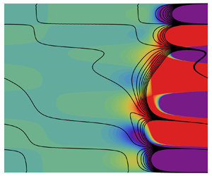
Figure 4. (a) Critical Rayleigh numbers for the onset of convective (dashed line) and absolute (solid line) instability as a function of the Péclet number for  $\beta =0$ and $Ge=0$. (b) Collision criterion (coloured lines) just before (blue), at (orange) and just after (green) the pinching point (large dot) for $\beta =0$, $Ge=0$, $Pe=50$ and $\omega _i=0$, with $(\alpha _r,\alpha _i) = (2.88674,-3.12176)$, where the dashed line represents the steepest ascent path followed by the pinching point since the onset of convective instability.
4.3.2. With internal heating: small Péclet numbers
The influence of viscous dissipation on the asymptotic disturbance behaviour is now discussed, focusing first on small Péclet numbers, namely  $Pe\leq 50$. Table 2 presents critical Rayleigh number, real frequency and complex wavenumber for a few given Péclet and Gebhart numbers at the onset of absolute instability. On one hand, throughflow still has a stabilising effect on the transition to absolute instability in the presence of viscous dissipation. On the other hand, viscous dissipation has a destabilising effect on this transition in the presence of throughflow. This is due to the fact that it acts as an internal heating mechanism and, hence, less external heating is required. Further insight can be gained using (3.13). According to this equation, throughflow effects are approximately $O(Pe)$ whereas viscous dissipation effects are approximately $O(Ge\,Pe^2)$, which explains why viscous dissipation effects only become relevant at large $Ge$ for these moderate $Pe$. Such a dimensional analysis also indicates that throughflow will eventually have a destabilising effect when it is large enough.
Table 2. Throughflow ( $Pe$) and viscous dissipation ( $Ge$) influence on the transition to absolute instability ( $\omega _i=0$).


Figure 5. Onsets of convective (small dashed line) and absolute instabilities for  $Ge=0.1$ and $Pe\leq 450$, showing saddle points (long dashed lines) competing for the role of pinching point (solid line). Red dots labelled (a–f) are evaluated at the critical points $(Pe,Ra)=(10,57.7822)$, $(100,413.001)$, $(206.2,857.197)$, $(300,728.532)$, $(373.2,402.244)$ and $(420,-58.0117)$, respectively.
Before proceeding any further, it is important to remind the reader about the Gebhart number magnitude. In most engineering applications,  $Ge\ll 1$. However, it is possible to reach $Ge \sim O(1)$ in some geophysical flows. This is the reason why such a range was used in table 2. Nevertheless, for the purposes of the present study, $Ge=0.1$ is assumed to be a reasonable upper bound in the following discussion.
4.3.3. With internal heating: large Péclet numbers
Focus is now switched to a larger Péclet number range, i.e.  $50 \le Pe \leq 450$. It is important to remind the reader that the Péclet number is the product of the Prandtl and Reynolds numbers. Since the former can have quite high values even for moderate values of the latter, such a large Péclet number range is indeed not uncommon. Furthermore, the influence of viscous dissipation on the time asymptotic disturbance behaviour is discussed in detail from this point for $Ge=0.1$, which has already been established as a reasonable upper bound for this parameter. Nevertheless, the disturbance behaviour at smaller $Ge$ values is summarised at the end of this subsection.
Figure 5 shows the onsets of convective (small dashed line) and absolute (solid line) instabilities over the aforementioned  $(Ge,Pe)$ parametric region, where three different saddle points (long dashed lines) compete for the role of pinching point. Their respective collision criterions (solid lines) are provided in figure 6 for the six $(Pe,Ra)$ critical points (red dots) shown in figure 5. The paths taken by all three saddle points in the complex streamwise wavenumber plane as the Péclet number varies between $0\leq Pe \leq 450$ are also shown (non-solid lines) in figure 6. As already illustrated in figure 1, it is important to note that the onset of convective instability is always destabilised by throughflow, so much so that the flow becomes convectively unstable even when heated from above for $Pe\geq 68.6575$ (Nield et al. Reference Nield, Barletta and Celli2011). The effect of throughflow on the onset of absolute instability, on the other hand, is significantly less straightforward. A single downstream propagating branch $\alpha ^+$ is involved in the collision that forms the pinching point for all Péclet numbers within $0\leq Pe \leq 450$. This collision, however, occurs against one of three different upstream propagating branches, namely $\alpha _1^{-}$, $\alpha _2^{-}$ and $\alpha _3^{-}$, within the same Péclet number range. Consider first scenario (a) from figures 5 and 6. This particular pinching point is formed by a collision between branches $\alpha ^+$ and $\alpha _1^{-}$ and called here mode 1. The other two saddle points are formed by collisions between upstream propagating branches and, hence, do not have any physical meaning. Mode 1 is the same transition mechanism observed in the absence of viscous dissipation, as shown in figure 4, where the latter two saddle points do not exist. A similar transition mechanism is observed in scenario (b) from figures 5 and 6. The only qualitative difference observed at this higher Péclet number is related to the wavenumber of the saddle points induced by viscous dissipation, whose real part is no longer zero. A further increase in the throughflow magnitude to $Pe=206.2$, however, leads to the emergence of a new transition mechanism. Scenario (c) from figures 5 and 6 show a codimension-two point where the traditional (convection dominated) and novel (viscous dissipation dominated) saddle points are equally unstable. In other words, branch $\alpha ^+$ collides simultaneously with branches $\alpha _1^{-}$ and $\alpha _2^{-}$. The latter collision, however, is called mode 2 here and is the one that leads to the pinching point at higher throughflow, as shown in scenario (d) from figures 5 and 6. Increasing the throughflow even further to $Pe\simeq 373.2$, on the other hand, leads to a new codimension-two point, but now between both novel viscous dissipation dominated saddle points, as shown in scenario (e) from figures 5 and 6. In other words, branch $\alpha ^+$ collides simultaneously with branches $\alpha _2^{-}$ and $\alpha _3^{-}$. This second viscous dissipation related collision is called here mode 3 and leads to the pinching point at higher throughflow, as shown in scenario ( f) from figures 5 and 6. There are more viscous dissipation related saddle points, but they only become relevant at higher Gebhart numbers, which are non-physical. Hence, they are not discussed. Finally, it is important to note that a linear stability analysis cannot provide additional information about either codimension-two point. Under either parametric condition, a nonlinear analysis is required to clarify the dynamical system behaviour.

Figure 6. Collision checks for the parametric conditions shown in figure 5 at (a)  $Pe=10$, where $(\alpha _r,\alpha _i) = (3.39332,-1.89382)$, (b) $Pe=100$, between branches $\alpha ^+$ and $\alpha _1^{-}$, where $(\alpha _r,\alpha _i) = (2.54770,-3.41712)$, (c) $Pe\simeq 206.2$ between branches $\alpha ^+$ and $\alpha _1^{-}$, where $(\alpha _r,\alpha _i) = (1.92771,-3.81869)$ and branches $\alpha ^+$ and $\alpha _2^{-}$, where $(\alpha _r,\alpha _i) = (3.14560,-6.65050)$, (d) $Pe=300$, between branches $\alpha ^+$ and $\alpha _2^{-}$, where $(\alpha _r,\alpha _i) = (2.68895,-6.76400)$, (e) $Pe\simeq 373.2$, between branches $\alpha ^+$ and $\alpha _2^{-}$, where $(\alpha _r,\alpha _i) = (2.15204,-7.06621)$, and branches $\alpha ^+$ and $\alpha _3^{-}$, where $(\alpha _r,\alpha _i) = (2.70854,-8.96509)$, and ( f) $Pe=420$, between branches $\alpha ^+$ and $\alpha _3^{-}$, where $(\alpha _r,\alpha _i) = (2.76478,-8.93637)$. The non-solid curves represent the paths taken by each saddle point (i.e. modes 1, 2 and 3) as the Péclet number varies.
Figures 7 and 8 show the disturbance streamlines and isotherms at the codimension-two points  $Pe \simeq 206.2$ and $\simeq 373.2$, respectively. Dashed (solid) lines stand for negative (positive) values in the streamline plots. Modes 1, 2 and 3 are clearly distinct from one another. Similarly to the typical cell pattern behaviour observed in convectively unstable conditions, higher order modes have a larger number of cells. They are concentrated in the downstream end of both figures because all three modes grow in space at the onset of absolute instability. Finally, it is also interesting to note that the cell pattern is closer to horizontal for mode 1 but closer to vertical for mode 3. This is related to the fact that the spatial growth rates are different for each mode, as shown in figure 6. In figure 7, $\alpha _i = -3.81869$ for mode 1 but $\alpha _i = -6.65050$ for mode 2. In figure 8, $\alpha _i = -7.06621$ for mode 2 and $\alpha _i = -8.93637$ for mode 3.

Figure 7. Stream function (a,c) and temperature (b,d) isolines for mode 1 (a,b) and mode 2 (c,d) at  $Pe\simeq 206.2$, i.e. at the first codimension-two point.

Figure 8. Stream function (a,c) and temperature (b,d) isolines for mode 2 (a,b) and mode 3 (c,d) at  $Pe\simeq 373.2$, i.e. at the second codimension-two point.
When  $Ge=0.1$, as shown in figure 5, the transition from convective to absolute instability for $Pe_C \simeq 414.651$ occurs when $Ra=0$. This means that transition is induced by internal heating alone, i.e. without external heating. In other words, viscous dissipation alone, without the influence of buoyancy effects, is responsible for the onset of absolute instability. Furthermore, when $Pe \ge Pe_C$, absolute instability occurs even in the presence of negative Rayleigh numbers. Under these conditions, a stable temperature stratification would be induced with $Ge=0$. Hence, the internal heating mechanism created by viscous dissipation is capable of inducing transition even in the presence of the stabilising external heating mechanism created by buoyancy. It turns out this critical Péclet number is induced by mode 3 and depends on the Gebhart number according to $Pe_C \simeq 41.9479/Ge$, since the mode 2 dependence is given by $Pe_C \simeq 43.3805/Ge$. Both correlations were obtained using nonlinear regression based on the data provided in tables 3 and 4, which also provides eigenvalues. The standard errors of both parameters are $2.32605\times 10^{-3}$ and $1.35113\times 10^{-3}$, respectively. These correlations imply that $Pe_C \rightarrow \infty \, (0)$ when $Ge \rightarrow 0 \, (\infty )$, which is expected since more (less) throughflow is required to make viscous dissipation important when the Gebhart number decreases (increases). Finally, this correlation also implies that the qualitative trends shown in figures 5–8 would be the same for different Gebhart numbers, although occurring at different Rayleigh and Péclet numbers, which has been confirmed but is not shown.
Table 3. Saddle point data at the onset of absolute instability when  $Ra=0$ as a function of the Gebhart number for mode 2.

Table 4. Same as table 3 but for mode 3.

5. Conclusions
The present paper has investigated the appearance of natural convection, as induced by temporal disturbance growth, in the otherwise forced convection in porous media. At any given throughflow (Péclet number), instability could be induced by internal (Gebhart number) and/or external (Rayleigh number) heating. Both modal (asymptotic) and non-modal (transient) linear mechanisms have been considered. A matrix-forming approach based on a continuous spectral method has been employed to solve the differential eigenvalue problem. On one hand, the modal analysis has been performed using the dispersion relation obtained from the determinant of the resulting matrix. Auxiliary dispersion relations were then obtained by applying the zero group velocity conditions to verify the possibility of modal growth in time through absolute instability. On the other hand, the non-modal analysis has been performed using both the SVD of this matrix as well as the condition number of the respective eigenvector matrix. They allowed us to verify the possibility of transient growth. The major findings of our study are summarised as follows:
(i) In the absence of viscous dissipation, i.e. when the Gebhart number is zero, the differential eigenvalue problem is self-adjoint. However, this is no longer true for positive Gebhart numbers. Hence, non-modal growth is possible.
(ii) Non-modal growth was found negligible for a wide range of Péclet, Gebhart and Rayleigh numbers. Hence, it is possible to infer that there is no transient growth. This is true for two- and three-dimensional disturbances.
(iii) In the absence of internal heating, modal growth does occur for strong enough external heating, although throughflow has a stabilising effect. In the presence of internal heating, however, this is only true for a weak enough throughflow.
(iv) For a moderate throughflow, internal heating drives modal growth, where throughflow has a destabilising effect. Absolute instability is possible even in the absence of external heating, i.e. at zero Rayleigh number.
(v) For strong throughflows, internal heating is capable of inducing modal growth even in the presence of external cooling from below. In other words, absolute instability occurs for negative Rayleigh numbers.
(vi) In the three cases mentioned above, namely weak, moderate and strong throughflows, modal growth is controlled by mode 1, 2 and 3, respectively.
(vii) Two codimension-two points separate these three cases when $Ge=0.1$. The first one, separating weak and moderate throughflows, is located at $Pe \simeq 206.2$ whereas the second one, separating moderate and strong throughflows, is located at $Pe \simeq 373.2$.
(viii) Internal heating due to viscous dissipation effects is responsible for the appearance of modes 2 and 3, becoming the dominant mechanism over external heating responsible for the onset of absolute instability at moderate and strong throughflows.
(ix) Transverse modes are responsible for all modal growths discussed here. This is true when either internal or external heating acts as the dominant mechanism.


Current research is simulating the fully nonlinear system of governing equations to investigate both codimension-two points, which mark the switch between external and internal heating dominated absolute instabilities, as well as the switch between both internal heating dominated absolute instabilities, as throughflow increases. Furthermore, the possibility of a spatial non-modal growth is also being investigated.
Funding
The authors would like to thank the Brazilian funding agency CAPES for the masters (at UFF) and doctorate (at UniBo) fellowships provided to the first author, which allowed the development of this work.
Declaration of interests
The authors report no conflict of interest.
Appendix A
This appendix contains GITT summation series convergence results for the modal analysis. Table 5 lists the saddle point at  $Pe=300$ and $Ge=0$ converging as the number of terms in the series increases. A single term is enough to converge these results essentially because the matrix formed by (3.13) becomes diagonal, i.e. the coefficients given by (3.13) become decoupled.
Table 5. Saddle point summation series convergence for  $Ge=0$ and $Pe=200$.

Tables 6–8 are equivalent to table 5 but for  $Ge=0.1$ and three different values of $Pe$, namely $Pe=200$, $300$ and $400$, respectively. Comparing tables 5 and 6 shows that a larger number of terms is required for convergence, which is caused by the stability problem no longer being diagonal due to the use of a positive Gebhart number. In addition, comparing tables 6, 7 and 8 indicates that a larger Péclet number slows down convergence, which is caused by the orthogonal basis function used in the integral transformation being diffusive in nature.
Table 6. Same as table 5 but for  $Ge=0.1$.

Table 7. Same as table 6 but for  $Pe=300$.

Table 8. Same as table 7 but for  $Pe=400$.

Appendix B
This appendix contains a description of the eigenvector matrix construction as well as the condition number convergence. The eigenvectors are constructed based on the integral transformation (3.1), where  $\tilde {w}_m$ comes from the solution of the integral transformed eigenvalue problem. To construct a matrix in which the columns are the eigenvectors it is necessary to transform the continuous dependence on $z$ into a discrete one. In that way, one can have a matrix in which the columns are the eigenvectors, and the rows represent the $z$ dependence of each one. The number of columns and rows are related with the number of terms used in the summation series truncation and the points used in the discretisation, respectively. Here, the discretisation of the $z$ component is based on a uniform grid spacing, which is given by $1/N_z$, where $N_z$ is the number of points used by the discretisation. The condition number calculations are then based on the condition number definition for a generic matrix $A$, namely
 \begin{equation} {\rm cond}(A) = \|A\|\,\|A^+\|, \end{equation}
where  $A^+$ is the pseudo-inverse of $A$. Tables 9 and 10 list the condition number convergence in terms of $N_t$ and $N_z$.
Table 9. Condition number convergence for  $Ge=0.1$, $Pe=200$, $\alpha =3$ and $N_z=10$.

Table 10. Same as table 9 but for  $N_t=7$.

The convergence of the non-modal results is assumed, based on both modal and eigenvector matrix condition number convergence. In other words, it is considered here that the transient growth analysis is convergent because both eigenvector and eigenvalue calculations are convergent.


