1 Introduction and objectives

Canonical shear flows, such as wakes, jets, shear layers and boundary layers, have received much attention because they are relatively simple examples that serve as building blocks for more complex flows. The wake in a density-stratified background is such a canonical flow whose importance stems from engineering, biological and geophysical applications, such as underwater submersibles, aerial vehicles, marine swimmers, wind turbines and flows past topographic features on land and under water. Our interest is in the wake of ocean submersibles that inevitably operate in a density-stratified background. Such wakes are almost always turbulent, with a Reynolds number, $Re=U_{b}L_{b}/\unicode[STIX]{x1D708}$, that is large, e.g. $Re\sim O(10^{4}{-}10^{7})$, and are subject to stratification whose strength is measured by a Froude number, $Fr=U_{b}/NL_{b}$, that takes values of $O(1{-}10^{2})$.

Turbulent wakes of axisymmetric bodies, when subject to stratification, are non-axisymmetric, inhomogeneous and multistage. Axisymmetry is broken as a result of gravity-suppressed vertical motion. Wake turbulence is inhomogeneous due to the spatial variation from the wake core to the wake boundary as well as streamwise ($x$) evolution. As the wake evolves in $x$, the relative strength of stratification increases even for constant $N$, since the ‘local Froude number’, $Fr_{H}=U_{0}/NL_{H}$, based on a local wake size ($L_{H}$) continually decreases. Therefore, the wake evolution is multistage, as was first described in Lin & Pao (Reference Lin and Pao1979) and later categorized by Spedding (Reference Spedding1997), who experimentally measured $U_{0}$ behind a towed sphere in a salt-stratified tank, and identified three-dimensional (3-D), non-equilibrium (NEQ) and quasi-two-dimensional (Q2D) stages in the evolution of $U_{0}$. Later, Meunier, Diamessis & Spedding (Reference Meunier, Diamessis and Spedding2006) pointed to a viscous three-dimensional (V3D) regime, a final stage of the evolution. While subsequent studies have confirmed the existence of these stages, quantitative results regarding regime characteristics and the transition points between successive regimes are not strictly consistent, and the applicability of these regimes to turbulence statistics is unclear.

During the initial 3-D stage, a stratified wake shows little effect of buoyancy and unstratified wake laws apply. For a high-$Re$ unstratified wake, classical theory (Tennekes & Lumley Reference Tennekes and Lumley1972; Townsend Reference Townsend1976) offers the power law $U_{0}\propto x^{-2/3}$ for the far wake. Later, George (Reference George, George and Arndt1989) proposed that $U_{0}\propto x^{-1}$ applies to a low-$Re$ wake. While these two scalings have been ‘found’ in early experiments and numerical simulations (see review by Johansson, George & Gourlay (Reference Johansson, George and Gourlay2003)), their universality is not clear. Evidence of axisymmetric wakes with power laws that do not conform to $U_{0}\propto x^{-2/3}$ has accumulated (e.g. Bonnier & Eiff Reference Bonnier and Eiff2002; Nedić, Vassilicos & Ganapathisubramani Reference Nedić, Vassilicos and Ganapathisubramani2013; de Stadler, Rapaka & Sarkar Reference de Stadler, Rapaka and Sarkar2014; Dairay, Obligado & Vassilicos Reference Dairay, Obligado and Vassilicos2015; Chongsiripinyo & Sarkar Reference Chongsiripinyo and Sarkar2017; Pal et al. Reference Pal, Sarkar, Posa and Balaras2017). Nedić et al. (Reference Nedić, Vassilicos and Ganapathisubramani2013) suggested that this contradiction can be explained if the inviscid dissipation estimate $\unicode[STIX]{x1D700}\sim u^{\prime 3}/l$, which is consistent with classical similarity analysis as applied to the turbulent kinetic energy (TKE) equation, is modified. Here, $u^{\prime }$ is the root-mean-square (r.m.s.) streamwise velocity fluctuation and $l$ is taken to be the wake width. It is also worth noting that a proportionality $u^{\prime }\sim U_{0}$ is assumed in the classical analysis. An alternative to the inviscid estimate is $\unicode[STIX]{x1D700}=C_{\unicode[STIX]{x1D700}}u^{\prime 3}/l$, where $C_{\unicode[STIX]{x1D700}}\sim Re_{Global}^{m}/Re_{Local}^{n}$, as discussed by Vassilicos (Reference Vassilicos2015); here, $Re_{Global}$ is a global Reynolds number based on inlet conditions, and $Re_{Local}$ is a local Reynolds number based on local velocity and length scales. This ‘non-equilibrium’ dissipation scaling has been tested in a variety of turbulent flows: decay of fractal-generated turbulence (Seoud & Vassilicos Reference Seoud and Vassilicos2007), a fractal-plate turbulent wake (Nedić et al. Reference Nedić, Vassilicos and Ganapathisubramani2013; Dairay et al. Reference Dairay, Obligado and Vassilicos2015) and a sphere wake (Chongsiripinyo, Pal & Sarkar Reference Chongsiripinyo, Pal and Sarkar2019).

Following the 3-D regime in stratified wakes is the NEQ regime. Here, the decay of $U_{0}$ slows down substantially and is close to $U_{0}\propto x^{-0.25}$ (Spedding Reference Spedding1997) in sphere-wake experiments. This is the regime whose dynamics allows a stratified wake to ‘survive longer’ than its unstratified counterpart. Brucker & Sarkar (Reference Brucker and Sarkar2010) attributed the slower decay of $U_{0}$ to the reduction of the mean-to-turbulence energy transfer by production, $P=-\langle u_{x}^{\prime }u_{z}^{\prime }\rangle \unicode[STIX]{x2202}_{z}\langle u_{x}\rangle$, an effect that was attributed to buoyancy-induced reduction of the correlation between $u_{x}^{\prime }$ and $u_{z}^{\prime }$. Following NEQ, the wake enters into the Q2D regime where $u_{h}^{\prime }\gg u_{z}^{\prime }$ (hence the ‘two-dimensional’ attribute). According to Spedding (Reference Spedding1997), the Q2D regime exhibits an increase in wake decay to $U_{0}\propto x^{-3/4}$, and the NEQ-to-Q2D transition takes place at $Nt_{b}=50$, where $t_{b}=x/U_{b}$. It is worth noting that the later studies of Brucker & Sarkar (Reference Brucker and Sarkar2010) and Diamessis, Spedding & Domaradzki (Reference Diamessis, Spedding and Domaradzki2011) find that the span of the NEQ regime increases with $Re$. The other distinct characteristic of the Q2D wake is the presence of horizontally large but vertically thin ‘pancake eddies’ at large time ($Nt_{b}\approx 250$) in experiments as well as simulations such as Brucker & Sarkar (Reference Brucker and Sarkar2010) and Chongsiripinyo, Pal & Sarkar (Reference Chongsiripinyo, Pal and Sarkar2017).

The progression of stratified wakes through each regime has become clearer owing to previous work. However, much of our later understanding derives from simulations that utilize the so-called temporal model (e.g. Gourlay et al. Reference Gourlay, Arendth, Fritts and Werne2001; Dommermuth et al. Reference Dommermuth, Rottman, Innis and Novikov2002; Diamessis, Domaradzki & Hesthaven Reference Diamessis, Domaradzki and Hesthaven2005; Brucker & Sarkar Reference Brucker and Sarkar2010; Diamessis et al. Reference Diamessis, Spedding and Domaradzki2011; de Stadler & Sarkar Reference de Stadler and Sarkar2012; Abdilghanie & Diamessis Reference Abdilghanie and Diamessis2013; Redford, Lund & Coleman Reference Redford, Lund and Coleman2015; among others). The temporal model invokes the Galilean transformation that relates time $T=x/U$ in the reference frame (implicitly moves with the body velocity $U$) of the simulation to distance ($x$) from the wake generator in the laboratory frame.

The temporal model has proved important to track wakes over a long time (equivalently, streamwise distance) and into the Q2D regime. However, temporal-model simulations are sensitive to the choice of initial conditions. Redford, Castro & Coleman (Reference Redford, Castro and Coleman2012) found that the early and intermediate development of the axisymmetric wake in the temporal model depends not only on whether coherent vortex rings are initially introduced, but also on their relative spacing. For example, both of the power-law exponents, $U_{0}\propto x^{-1}$ and $x^{-2/3}$, were found to arise from two initial conditions that differ by the presence of coherent vortex rings. Interestingly, Redford et al. (Reference Redford, Lund and Coleman2015) found the canonical rate of decay $U_{0}\propto x^{-2/3}$ despite the statistics not being fully self-similar. To the best of our knowledge, the early/intermediate development of case VR (with vortex rings) from Redford et al. (Reference Redford, Lund and Coleman2015) is the only simulation utilizing the temporal-model approximation that produces $U_{0}\propto x^{-1}$.

Body-inclusive simulations naturally capture flow separation and vortex shedding from the body and, importantly, avoid the uncertainty introduced by assumed initial conditions in the temporal model. The disadvantage, however, is the high computational cost of boundary-layer resolution so that a long domain that captures all the three regimes (3-D, NEQ, Q2D) becomes infeasible for a high-$Fr$ wake. A work-around is to continue a body-inclusive simulation with separate simulations that can be performed with a temporal model (Pasquetti Reference Pasquetti2011) or a spatially evolving model (VanDine, Chongsiripinyo & Sarkar Reference VanDine, Chongsiripinyo and Sarkar2018).

Body-inclusive simulations of stratified turbulent wakes are recent. Such simulations include a $Re=10^{3}$ sphere by Orr et al. (Reference Orr, Domaradzki, Spedding and Constantinescu2015) and $Re=3700$ sphere wakes at $Fr<O(1)$ (Pal et al. Reference Pal, Sarkar, Posa and Balaras2016) and $Fr=O(1)$ (Pal et al. Reference Pal, Sarkar, Posa and Balaras2017). These simulations have captured vortex-shedding modes (Orr et al. Reference Orr, Domaradzki, Spedding and Constantinescu2015), oscillatory modulation of the wake by body-generated lee waves (Pal et al. Reference Pal, Sarkar, Posa and Balaras2017), the re-energization of fluctuations at low $Fr$ (Pal et al. Reference Pal, Sarkar, Posa and Balaras2016; Ortiz-Tarin, Chongsiripinyo & Sarkar Reference Ortiz-Tarin, Chongsiripinyo and Sarkar2019) and the associated change in vortex dynamics (Chongsiripinyo et al. Reference Chongsiripinyo, Pal and Sarkar2017). These features of the flow could not have been captured with a temporal model. The statistics to be presented in this work demonstrate the impact of these features on wake evolution.

Stratified wakes are inhomogeneous turbulent flows with mean shears that are subject to stratification. There has been much work – a non-exhaustive list is Lilly (Reference Lilly1983), Billant & Chomaz (Reference Billant and Chomaz2001), Riley & de Bruyn Kops (Reference Riley and de Bruyn Kops2003), Brethouwer et al. (Reference Brethouwer, Billant, Lindborg and Chomaz2007), Kimura & Herring (Reference Kimura and Herring2012), Maffioli & Davidson (Reference Maffioli and Davidson2016) and de Bruyn Kops & Riley (Reference de Bruyn Kops and Riley2019) – in the related problem of fluctuations that evolve without mean shear in a stratified fluid. The interest is in the behaviour of ‘stratified turbulence’ defined as fluctuations that have low values of Froude number ($Fr_{h}$ defined by (3.4) is <1) but the Reynolds number is not low ($Re_{b}$ defined by (3.3) is >1).

A limitation of the previous body-inclusive simulations is that $Re=O(10^{3})$ was not sufficiently large to have a developed region of stratified turbulence with fluctuations at low Froude number and high Reynolds number. Furthermore, wakes with high $Fr$ (${>}O(10)$) were not simulated. We are therefore motivated to simulate wakes at a higher $Re=5\times 10^{4}$ and over a wide range of stratifications, $\{Fr=2,10,50,\infty \}$. We will explore links between the findings in our simulations and those in the general topic of stratified turbulence. Furthermore, we consider a disk rather than a sphere to broaden the stratified-wake literature. The unstratified $Fr=\infty$ case allows examination of power laws at a higher $Re$ than in prior simulations and assesses the possibility of non-canonical power laws for $U_{0}$ and $L$.

The primary objective of the present study is to improve our understanding of the behaviour of relatively high-$Re$ stratified wakes. In particular, we consider the following questions. What are the power laws that are satisfied by characteristic velocities/length scales as the wake progresses? Are there differences between the progression of mean and r.m.s. turbulence as they react to stratification? How does the development of wake turbulence relate to the broader area of stratified turbulence decay? Lastly, what are the reasons underlying the slower decay of the wake in the NEQ regime?

The numerical set-up and the parameters of the simulated cases are given in § 2. Definitions used in the analysis and interpretation of results are given in § 3. Presentation of the results begins with § 4, which introduces the effect of stratification by visual contrasts among the different cases. Section 5 reports on the evolution of centreline values of the mean and the three r.m.s. components for each of the cases, separately. Section 6 presents a consolidated picture of the three stratified cases in phase space. We discuss links with previous work on regimes (characterization and transitions) of stratified wakes and stratified turbulence in both §§ 5 and 6. Section 7 concerns the behaviour of two distinct wake sizes; one is derived from profiles of $U_{0}$ and the other is based on TKE. Section 8 discusses the progression of area-integrated kinetic and potential energy in stratified wakes and contrasts with the unstratified wake. Section 9 delves deeper into the evolution of mean kinetic energy (MKE) and TKE through their budgets. Section 10 discusses possible scaling laws for the dissipation ($\unicode[STIX]{x1D700}$) of TKE. We end with a summary and conclusions in § 11.

2 Numerical simulations

We address the questions introduced in § 1 with large-eddy simulations (LES) of flow past a circular solid disk placed perpendicular to the uniform free stream. The background is taken to have a uniform stratification. These body-inclusive simulations of flow into the far wake (up to $x/D=125$) are at a relatively high $Re$ of 50 000 and computationally intensive because of the necessity of resolving the separated flow at the body and the turbulent recirculation region. The following non-dimensional filtered Navier–Stokes equations under the Boussinesq assumption for density effects along with the filtered advection–diffusion equation for density are numerically solved:

(2.1)$$\begin{eqnarray}\displaystyle & \displaystyle \text{continuity:}\quad \unicode[STIX]{x2202}_{i}u_{i}=0, & \displaystyle\end{eqnarray}$$

(2.2)$$\begin{eqnarray}\displaystyle & \displaystyle \text{momentum:}\quad \unicode[STIX]{x2202}_{t}u_{i}+u_{j}\unicode[STIX]{x2202}_{j}u_{i}=-\unicode[STIX]{x2202}_{i}p+Re^{-1}\unicode[STIX]{x2202}_{j}[(1+\unicode[STIX]{x1D708}_{s}/\unicode[STIX]{x1D708})\unicode[STIX]{x2202}_{j}u_{i}]-Fr^{-2}\unicode[STIX]{x1D70C}_{d}\unicode[STIX]{x1D6FF}_{i3}, & \displaystyle\end{eqnarray}$$

(2.3)$$\begin{eqnarray}\displaystyle & \displaystyle \text{density:}\quad \unicode[STIX]{x2202}_{t}\unicode[STIX]{x1D70C}+u_{j}\unicode[STIX]{x2202}_{j}\unicode[STIX]{x1D70C}=(RePr)^{-1}\unicode[STIX]{x2202}_{j}[(1+\unicode[STIX]{x1D705}_{s}/\unicode[STIX]{x1D705})\unicode[STIX]{x2202}_{j}\unicode[STIX]{x1D70C}]. & \displaystyle\end{eqnarray}$$

The symbol $\unicode[STIX]{x2202}_{i}$ denotes a spatial derivative with respect to $x_{i}$, where $i=1,2,3$ respectively refer to streamwise ($x$), lateral ($y$) and vertical ($z$) directions with $u_{x}$, $u_{y}$ and $u_{z}$ the corresponding velocities. The governing equations are non-dimensionalized with the following parameters: the background free-stream velocity ($U_{b}$), the disk diameter referred as the body length scale ($L_{b}$), advection time ($L_{b}/U_{b}$), dynamic pressure ($\unicode[STIX]{x1D70C}_{0}U_{b}^{2}$) and characteristic change in background density deviation across the body ($-L_{b}\unicode[STIX]{x2202}_{3}\unicode[STIX]{x1D70C}_{b}$). Under the Boussinesq approximation, the density deviation from its equilibrium alters the momentum equation only through the last term on the right-hand side of (2.2). Here $\unicode[STIX]{x1D6FF}_{i3}$ is the Dirac delta function. The density is decomposed into a constant reference density ($\unicode[STIX]{x1D70C}_{0}$), the linearly varying deviation of the background $\unicode[STIX]{x1D70C}_{b}(x_{3})$ and the flow-induced deviation, $\unicode[STIX]{x1D70C}_{d}(x_{i},t)$, as follows:

(2.4)$$\begin{eqnarray}\displaystyle \text{density decomposition:}\quad \unicode[STIX]{x1D70C}(x_{i},t)=\unicode[STIX]{x1D70C}_{0}+\unicode[STIX]{x1D70C}_{b}(x_{3})+\unicode[STIX]{x1D70C}_{d}(x_{i},t). & & \displaystyle\end{eqnarray}$$

Note that $\unicode[STIX]{x1D70C}_{d}(x_{i},t)=\langle \unicode[STIX]{x1D70C}_{d}(x_{i},t)\rangle +\unicode[STIX]{x1D70C}_{d}^{\prime }(x_{i},t)$, where $\langle \unicode[STIX]{x1D70C}_{d}(x_{i},t)\rangle$ is not necessarily zero but takes a value of $\unicode[STIX]{x2202}_{n}\langle \unicode[STIX]{x1D70C}_{d}(x_{i},t)\rangle =-\unicode[STIX]{x2202}_{n}\unicode[STIX]{x1D70C}_{b}(x_{3})$ at a solid surface; $n$ is a surface normal direction. Background density and static linear variation are absorbed into the modified pressure. The body Reynolds number is $Re=U_{b}L_{b}/\unicode[STIX]{x1D708}$, where $U_{b}$ is the free-stream velocity, $L_{b}$ is the characteristic length taken to be the disk diameter, and $\unicode[STIX]{x1D708}$ is the fluid kinematic viscosity. The body Froude number $Fr=U_{b}/NL_{b}$ is the ratio of buoyancy time scale to the characteristic advection time scale, $L_{b}/U_{b}$; here, $N$ is the constant buoyancy frequency defined by $N^{2}=-(g/\unicode[STIX]{x1D70C}_{o})\unicode[STIX]{x2202}_{3}\unicode[STIX]{x1D70C}_{b}$. The background is stably stratified if $\unicode[STIX]{x2202}_{3}\unicode[STIX]{x1D70C}_{b}$ is negative, as is the case here. The disk thickness of $0.01L_{b}$ is small. The Prandtl number, $Pr=\unicode[STIX]{x1D708}/\unicode[STIX]{x1D705}$, that is, the ratio of velocity and density (temperature) diffusivities, is assumed to be unity. Additional variables from small unresolved scales are subgrid kinematic viscosity, $\unicode[STIX]{x1D708}_{s}$, and density diffusivity, $\unicode[STIX]{x1D705}_{s}$. The Prandtl number based on these subgrid variables is also assumed to be unity. The study of the Prandtl-number effects in a stratified wake can be found in de Stadler, Sarkar & Brucker (Reference de Stadler, Sarkar and Brucker2010).

Since the turbulent wake under weak-to-intermediate stratification is quasi-axisymmetric in the 3-D and in the early-NEQ regimes, a cylindrical coordinate system is employed. The choice of cylindrical coordinates allows efficient distribution of grid points especially from the core to the wake periphery. Spatial numerical derivatives are obtained with second-order-accurate central differences, while temporal marching is done with a fractional-step method that combines a third-order Runge–Kutta explicit scheme with the second-order Crank–Nicolson implicit scheme. To alleviate stiffness of the discretized system, especially near the coordinate streamwise axis, implicit marching is performed for viscous and advection terms (both velocities and density) that involve spatial discretization in the azimuthal direction. In the fractional-step method, the Poisson equation is formed by taking the divergence of the momentum equation for predicted velocity. The periodic boundary condition in the azimuthal direction transforms the discretized Poisson equation into inversion of a pentadiagonal matrix. The pentadiagonal matrix system is then inverted using a direct solver (Rossi & Toivanen Reference Rossi and Toivanen1999). The disk is represented by the immersed boundary method of Balaras (Reference Balaras2004) and Yang & Balaras (Reference Yang and Balaras2006). Kinematic subgrid viscosity, $\unicode[STIX]{x1D708}_{s}$, is obtained using the eddy viscosity model of Germano et al. (Reference Germano, Piomelli, Moin and Cabot1991), a variant of the dynamic Smagorinsky model (Smagorinsky Reference Smagorinsky1963). The coefficient $C$, as in $\unicode[STIX]{x1D708}_{t}=C\widetilde{\unicode[STIX]{x1D6E5}}^{2}|\widetilde{S}|$, where $\widetilde{\unicode[STIX]{x1D6E5}}^{3}=V$ is a measure of the local cell volume and $|\widetilde{S}|$ is the instantaneous strain-rate magnitude of filtered velocity, is dynamically computed using a method of Lilly (Reference Lilly1992) that takes the cumulative average of $C$ along flow trajectories with an exponential weighting function chosen to give more weight to recent times in flow history. Boundary conditions at the inlet and outlet of the domain are Dirichlet inflow and Orlanski-type convective outflow, $\unicode[STIX]{x2202}_{t}\unicode[STIX]{x1D719}+C\unicode[STIX]{x2202}_{1}\unicode[STIX]{x1D719}=0$. The magnitude of convective velocity, $C$, is set at $U_{b}$. Note that a localized mean value of $C$ as an alternative to $U_{b}$ is tested with negligible consequence. The Neumann condition is used at the outer radial boundary. Unlike Chongsiripinyo & Sarkar (Reference Chongsiripinyo and Sarkar2017) and Pal et al. (Reference Pal, Sarkar, Posa and Balaras2017), who use a ‘sponge’ region for all of their cases to absorb internal gravity waves, the domain’s radial extent in this present study is enlarged to $80L_{b}$, allowing free propagation of internal gravity waves while minimizing reflection from the boundary without artificially adjusting the far field to a background state. In the present study, a sponge region of a Rayleigh-damping functional form, which gradually relaxes the velocities and density to their respective values at the boundaries, is applied only in the F02 case.

Table 1. Physical and numerical parameters used in the simulations: $N_{r}$, $N_{\unicode[STIX]{x1D703}}$ and $N_{x}$ are the number of nodes in the radial, azimuthal and streamwise directions, respectively; the streamwise domain length is split into downstream ($L_{x}^{+}$) and upstream ($L_{x}^{-}$) portions; the domain length is $L_{x}=L_{x}^{-}+L_{x}^{+}$. Note that all lengths are normalized by the diameter, $L_{b}$, of the disk.

Parameters of the simulations are given in table 1. The distribution of the computational grid is optimized on the basis of the unstratified case (UNS) where the turbulent dissipation rate is known to decay as $\unicode[STIX]{x1D700}\propto x^{-m}$, $m\leqslant 5/2$, in the self-similar solution (George Reference George, George and Arndt1989), thus leading to an estimate of the Kolmogorov length. The streamwise-dependent radial distribution of $\unicode[STIX]{x1D700}$ is estimated from the direct numerical simulation (DNS) of Dairay et al. (Reference Dairay, Obligado and Vassilicos2015) and the LES of Chongsiripinyo & Sarkar (Reference Chongsiripinyo and Sarkar2017). The resulting number of grid points for the weakly stratified cases is 624 million cells. In the unstratified wake, $\unicode[STIX]{x0394}x/\unicode[STIX]{x1D702}$ is at worst ${\approx}17$ near the centreline at $x/L_{b}\approx 2.5$; here $\unicode[STIX]{x1D702}$ is the Kolmogorov scale calculated directly from the turbulent dissipation rate by $\unicode[STIX]{x1D702}=(Re^{3}\unicode[STIX]{x1D700})^{-1/4}$. Beyond approximately $x/L_{b}=10$, the centreline $\unicode[STIX]{x0394}x/\unicode[STIX]{x1D702}$ is smaller than 10 and gradually decreases to approximately 6 at $x/L_{b}=125$. The distributions of $\unicode[STIX]{x0394}x/\unicode[STIX]{x1D702}$ and $\unicode[STIX]{x0394}r/\unicode[STIX]{x1D702}$ are given in figure 1. To ensure adequacy of the high spatial resolution utilized here, a grid sensitivity study is conducted. In the grid sensitivity study, the grid spacings in the azimuthal and streamwise directions are both increased by a factor of 2 ($N_{\unicode[STIX]{x1D703}}=128$ and $N_{x}=2304$). None of the qualitative or quantitative results on wake statistics are altered. The approximate time step for all the cases lies in the range $(2{-}9)\times 10^{-4}L_{b}/U_{b}$. Statistics are collected over an averaging time ($T$) during a statistically steady state determined by convergence of moving-window averages of centreline streamwise and radial velocities at $x/L_{b}=100$. The steady state is reached after an initial transient that takes approximately two flow-through times. For the unstratified case, we use an averaging time of $T=500L_{b}/U_{b}$ after the transient has subsided. The effect of averaging time on the statistics is found to be small to negligible as the averaging time is changed from one to two flow-through times. The CPU usage, between 750 000 and 10⁶ core hours distributed over 512 cores for each case, is large because of the long integration time required to reach statistical steady state and then obtain converged statistics. The averaged drag coefficient in the unstratified case is found to be $C_{d}=1.145$, comparable to the value of $C_{d}=1.12$ in Fail, Eyre & Lawford (Reference Fail, Eyre and Lawford1959).

Figure 1. Grid quality. (a) Streamwise variation of non-dimensional streamwise grid spacing. (b) Radial profiles of non-dimensional radial grid spacing. The Kolmogorov length scale, $\unicode[STIX]{x1D702}=(\unicode[STIX]{x1D708}^{3}/\unicode[STIX]{x1D700}_{k})^{1/4}$, is computed using the rate of TKE dissipation ($\unicode[STIX]{x1D700}_{k}$) of the unstratified wake.

3 Analysis and interpretation

3.1 Statistics

Once statistical steady state is reached, the dependent variables are Reynolds-decomposed, $\unicode[STIX]{x1D719}=\langle \unicode[STIX]{x1D719}\rangle +\unicode[STIX]{x1D719}^{\prime }$, where $\unicode[STIX]{x1D719}$ is an instantaneous realization. Representing an ensemble average, the angle bracket $\langle \cdot \rangle$ denotes an appropriate averaging operator that involves averaging in all applicable homogeneous directions. Simulated in a spatially evolving domain, the turbulent wake in a homogeneous fluid is statistically homogeneous in time and in the azimuthal direction. The stratified wake is statistically homogeneous in time and is statistically symmetric across vertical and horizontal centre planes, $\langle \unicode[STIX]{x1D719}\rangle (x,y,z)=\langle \unicode[STIX]{x1D719}\rangle (x,\pm y,\pm z)$. The other type of statistic is obtained from cross-wake area integration indicated by braces $\{\cdot \}$,

(3.1)$$\begin{eqnarray}\{\unicode[STIX]{x1D719}\}(x)=\int _{0}^{2L_{k}(x,\unicode[STIX]{x1D703})}\unicode[STIX]{x1D719}(x,r,\unicode[STIX]{x1D703})\,\text{d}A,\end{eqnarray}$$

where the wake width ($L_{k}$) is described in § 3.2 and $\text{d}A=\unicode[STIX]{x0394}\unicode[STIX]{x1D703}r\,\text{d}r$ with $\unicode[STIX]{x0394}\unicode[STIX]{x1D703}=2\unicode[STIX]{x03C0}/N_{\unicode[STIX]{x1D703}}$. In order to include only wake turbulence and exclude internal wave contributions, a small integral number ($2L_{K}$) of wake widths is chosen for the radial limits of the integral. Lee waves, especially at intermediate stratification, generated by a wake generator can propagate considerably into the far field and we prefer to exclude the far field in the area integral.

3.2 Mean and turbulent length scales

In a homogeneous fluid, an axisymmetric half-length $L$ measures an azimuthally averaged distance from the centreline to a position where the streamwise mean velocity deficit is reduced to half of its centreline value, $U_{0}|_{r=L}=U_{0}|_{r=0}/2$. The other half-length, $L_{k}$, is based on profiles of the TKE, $K=\langle u_{i}^{\prime }u_{i}^{\prime }\rangle /2$, as opposed to $U_{0}$, taking $K|_{r=L_{k}}=K|_{r=0}/2$. In a stratified fluid, horizontal and vertical length scales are defined separately but again based on $U_{0}$ and $K$ profiles, and denoted as

(3.2)$$\begin{eqnarray}\displaystyle L_{H},\quad L_{V},\quad L_{Hk},\quad L_{Vk}. & & \displaystyle\end{eqnarray}$$

Here, the horizontal width ($L_{H}$) and vertical height ($L_{V}$) represent half-lengths in the lateral ($y$) and vertical ($z$) directions based on $U_{0}$, while $L_{Hk}$ and $L_{Vk}$ are derived from profiles of the TKE. Since $U_{0}$ and $K$ are obtained from the $\langle \cdot \rangle$ operator, a half-length is calculated based on an appropriately averaged ensemble. Note that, at steady state of all cases, although instantaneous wakes can meander around a mean position, the centreline peak values of $U_{0}$ and $K$ remain close to the axis of the cylindrical grid.

The turbulent integral length scale is not easy to calculate in a spatially evolving stratified wake where spatial homogeneity is absent. We use the wake width ($L_{Hk}$) as a surrogate for the horizontal integral length scale. The turbulent vertical length scale, $l_{v}$, is calculated along the centreline and its method of calculation is adopted from Riley & de Bruyn Kops (Reference Riley and de Bruyn Kops2003) as $l_{v}^{2}=\langle u_{x}^{\prime 2}+u_{y}^{\prime 2}\rangle /\langle (\unicode[STIX]{x2202}_{z}u_{x}^{\prime })^{2}+(\unicode[STIX]{x2202}_{z}u_{y}^{\prime })^{2}\rangle$. The quantity, $l_{v}$, has dynamic significance to shear instability. As shown by the scaling analysis of Riley & de Bruyn Kops (Reference Riley and de Bruyn Kops2003), $Fr_{v}=u_{h}^{\prime }/Nl_{v}$ defined using $l_{v}$ is proportional to ${Ri_{v}}^{-1/2}$, where $Ri_{v}$ is the Richardson number of the fluctuating shear in the flow.

3.3 Reynolds numbers and Froude numbers

The buoyancy Reynolds number ($Re_{b}$), the horizontal-motion Reynolds number ($Re_{h}$) and the microscale Reynolds number ($Re_{\unicode[STIX]{x1D706}}$) are defined as

(3.3a-c)$$\begin{eqnarray}Re_{b}=\frac{\unicode[STIX]{x1D700}_{k}}{\unicode[STIX]{x1D708}N^{2}},\quad Re_{h}=\frac{u_{h}^{\prime }L_{Hk}}{\unicode[STIX]{x1D708}},\quad Re_{\unicode[STIX]{x1D706}}=\frac{u_{x}^{\prime }\unicode[STIX]{x1D706}}{\unicode[STIX]{x1D708}},\end{eqnarray}$$

where $u_{h}^{\prime }=(u_{x}^{\prime 2}+u_{y}^{\prime 2})^{1/2}$ is the r.m.s. horizontal velocity fluctuation and $\unicode[STIX]{x1D706}$ is the Taylor microscale defined by $\unicode[STIX]{x1D706}^{2}=15\unicode[STIX]{x1D708}u_{x}^{\prime 2}/\unicode[STIX]{x1D700}_{k}$, with $\unicode[STIX]{x1D700}_{k}=\unicode[STIX]{x1D708}\langle \unicode[STIX]{x2202}_{j}u_{i}^{\prime }\unicode[STIX]{x2202}_{j}u_{i}^{\prime }\rangle +\unicode[STIX]{x1D708}\langle \unicode[STIX]{x2202}_{j}u_{i}^{\prime }\unicode[STIX]{x2202}_{i}u_{j}^{\prime }\rangle -\langle \unicode[STIX]{x1D70F}_{ij}^{s}\unicode[STIX]{x2202}_{j}u_{i}\rangle$ the rate of TKE dissipation. The mean vertical Froude number $(Fr_{V})$, the mean horizontal Froude number $(Fr_{H})$, the turbulent vertical Froude number $(Fr_{v})$ and the turbulent horizontal Froude number $(Fr_{h})$ are defined as follows:

(3.4a-d)$$\begin{eqnarray}Fr_{V}=\frac{U_{0}}{NL_{V}},\quad Fr_{H}=\frac{U_{0}}{NL_{H}},\quad Fr_{v}=\frac{u_{h}^{\prime }}{Nl_{v}},\quad Fr_{h}=\frac{u_{h}^{\prime }}{NL_{Hk}}.\end{eqnarray}$$

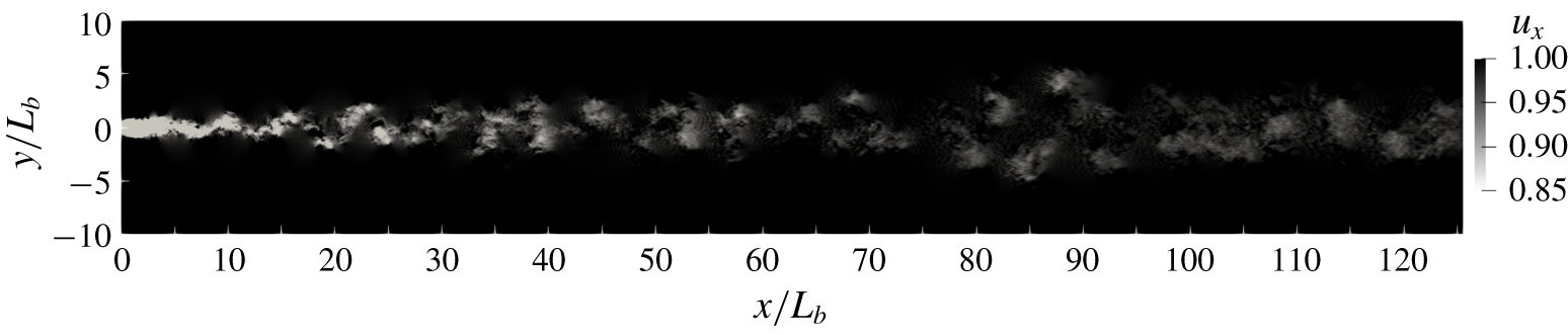
Figure 2. Snapshot of the streamwise velocity for the unstratified wake.

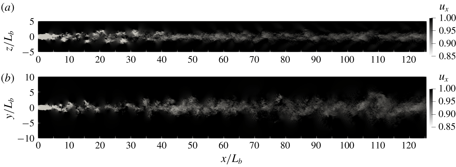
Figure 3. Case F10. Snapshot of the streamwise velocity in a vertical cut (a) and in a horizontal cut (b).

Figure 4. Case F02. Caption as in figure 3.

4 Visualization

Before considering the detailed analysis of wake statistics, we begin with a visualization that contrasts flow structures of the stratified wakes with those under unstratified conditions. Snapshots of the streamwise velocity ($u_{x}$) for the $Fr=\infty$, $10$ and $2$ wakes are shown in figures 2, 3 and 4, respectively. The body moving through the background leaves its imprint, which grows and lasts for a long distance, with its visual presentation being strongly dependent on the strength of stratification. When the stratification is weak ($Fr=10$), the near wake remains relatively unchanged relative to $Fr=\infty$ but the anisotropy between vertical and horizontal cuts is readily apparent in the intermediate and far wakes. When the stratification is strong ($Fr=2$), the wake quickly responds to the background stratification; even the near wake is vertically contracted and the intermediate/far wake is more coherent than at $Fr=\infty$. As buoyancy forces become relatively stronger, characterized by the decreased local Froude number, the far wake of the $Fr=10$ case behaves similarly to the near wake of the $Fr=2$ case by becoming horizontally wide but vertically thin. In fact, the $Fr=2$ and $Fr=10$ wakes are qualitatively equivalent if we compare the two at a normalized distance given by $(x/L_{b})Fr^{-1}=Nt_{b}$. This aspect will be quantitatively elaborated in §§ 5 and 6. As vertical motions become progressively suppressed, the wakes become increasingly two-dimensional, with the appearance of horizontal waviness that drives the formation of large-scale horizontal but vertically thin ‘pancake’ eddies that will emerge later in the Q2D regime.

Figure 5. Unstratified wake. Evolution of centreline values of mean streamwise velocity deficit ($U_{0}$), r.m.s. velocity fluctuation (streamwise $u_{x}^{\prime }$, spanwise $u_{y}^{\prime }$, vertical $u_{z}^{\prime }$) and turbulent velocity ($K^{1/2}$). The inset shows the evolution of turbulence velocity quantities normalized with the local $U_{0}(x)$.

5 Evolution of mean deficit velocity and turbulence intensities

Centreline values of mean streamwise velocity deficit ($U_{0}$) and r.m.s. velocity fluctuations in the streamwise ($u_{x}^{\prime }$), spanwise ($u_{y}^{\prime }$) and vertical ($u_{z}^{\prime }$) directions are shown in figure 5 for the unstratified wake. The initial increase of $U_{0}$ in the recirculation zone to exceed the free-stream velocity ($U_{b}$) is accompanied by an increase in all r.m.s. components signifying the establishment of turbulence. The r.m.s. fluctuations peak at $x/L_{b}\approx 2.5$, which lies in the recirculation region. The $U_{0}/U_{b}$ value decays over $2\leqslant x/L_{b}\leqslant 10$ with a rate that gradually decreases with increasing $x$. The subsequent evolution of $U_{0}$ in figure 5 reveals a break in slopes at $x/L_{b}\approx 65$ that separates two stages with different power-law exponents. The first stage of $10<x/L_{b}<65$ exhibits approximately $U_{0}\propto x^{-0.9}$ while the second stage of $65<x/L_{b}<125$ satisfies $U_{0}\propto x^{-0.6}$, close to the classical $U_{0}\propto x^{-2/3}$ behaviour. A similar transition between two different power laws was found by Dairay et al. (Reference Dairay, Obligado and Vassilicos2015) in the axisymmetric wake of a fractal plate. They identified $U_{0}\propto x^{-1}$ (an exponent of -0. 94 in their $Re=5000$ DNS and -1. 03 in their $Re=50\,000$ experiment) for $10<x/L_{b}<50$ that transitions to a different power law reported as $U_{0}\propto x^{-0.81}$ in the $Re=5000$ DNS. In our previous simulations of sphere wakes, namely DNS at $Re=3700$ by Pal et al. (Reference Pal, Sarkar, Posa and Balaras2017) and LES at $Re=10\,000$ by Chongsiripinyo et al. (Reference Chongsiripinyo, Pal and Sarkar2019), $U_{0}$ showed behaviour close to $x^{-1}$ scaling. Although it is tempting to attribute the $x^{-1}$ power law of $U_{0}$ to low-$Re$ viscous decay (George Reference George, George and Arndt1989), that is not the case. As we will show later during the analysis of MKE, the turbulent production that acts as a sink of MKE is much larger in magnitude than the viscous dissipation term in the MKE equation. Furthermore, the microscale Reynolds number, which varies between $Re_{\unicode[STIX]{x1D706}}=200$ at $x/D=10$ and $Re_{\unicode[STIX]{x1D706}}=120$ at $x/D=100$, is not small.

In contrast to $U_{0}$, the behaviour of the turbulent velocity scale ($K^{1/2}$) does not break into two separate power laws. The decay of $K^{1/2}$ (green circles in figure 5) is found to be $K^{1/2}\propto x^{-0.71}$, close to $x^{-2/3}$ from $x/L_{b}=10$ to the end of the computational domain. Thus, the mean velocity scale in the intermediate wake ($10<x/L_{b}<65$) decays with a different power-law exponent (-0. 9 as shown in figure 5) than the exponent satisfied by the turbulence velocity scale. Similarity theory for the turbulent wake (Tennekes & Lumley Reference Tennekes and Lumley1972) assumes the same velocity scale for both mean and turbulence. In the present simulation, it is only beyond $x/L_{b}=65$ that the power-law exponents for $U_{0}$ and $K^{1/2}$ become similar and close to the classical value of - 2/3. Near-wake turbulence is found to be anisotropic, with $u_{x}^{\prime }$ substantially smaller than $u_{y}^{\prime }$ and $u_{z}^{\prime }$ near the body; however, the r.m.s. velocity components (inset of figure 5) become more isotropic for $x/D>40$.

Figure 6. Case F50. (a) Evolution of centreline values of mean streamwise velocity deficit ($U_{0}$), r.m.s. velocity fluctuation (streamwise $u_{x}^{\prime }$, spanwise $u_{y}^{\prime }$, vertical $u_{z}^{\prime }$) and turbulent velocity ($K^{1/2}$). Unstratified case also shown for comparison with $U_{0}$ as dashed black line and $K^{1/2}$ as dashed green line. (b) Quantities normalized by the corresponding unstratified-wake value at the same $x/L_{b}$ (symbols and black solid line are as in panel (a)). (c) Quantities normalized by $U_{0}$. Symbols and black solid line are as in panel (a).

The behaviour of $U_{0}$ in case F50 (figure 6a) shows little deviation from the UNS case until $x/L_{b}\simeq 50$ or $Nt_{b}\simeq 1$, consistent with theoretical arguments such as given by Riley & Lelong (Reference Riley and Lelong2000) that it takes a time interval of $Nt\sim 1$ for buoyancy forces to become comparable to inertial forces in a flow that originates with weak buoyancy effects. Figure 6 emphasizes the importance of $Nt_{b}=1$ by showing that $U_{0}/U_{0\infty }$ (figure 6b) abruptly increases and $u^{\prime }/U_{0}$ (figure 6c) reaches the peak at $Nt_{b}\approx 1$. Here, $U_{0\infty }$ denotes the centreline deficit in the UNS case. Figure 6(b) also shows that stratification increases the rate of decay of $U_{0}$ as early as $x/L_{b}=10$ or $Nt_{b}=0.2$ (observe that $U_{0}/U_{0\infty }$ starts decreasing around $x/L_{b}=10$). Thus, there is a mild effect of buoyancy in the weakly stratified wake before $Nt_{b}=1$. Buoyancy increases the decay rate of $K^{1/2}$ (green circles) relative to the unstratified case (dashed green line). Figure 6(b) shows that all three turbulence components in F50 are reduced with respect to UNS, but the difference relative to UNS is smaller than that in $U_{0}$. The delay in the turbulence response to stratification in comparison to the mean velocity deficit will be more apparent in the F10 case and the reason for this delay will be made clear in the discussion of the F02 case.

Figure 7. Case F10. Caption as in figure 6.

In the F10 case (figure 7), buoyancy forces become comparable with inertial forces at a location closer to the body relative to F50 but at a similar value of $Nt_{b}$. The $U_{0}$ value deviates from the unstratified case at $x/L_{b}\approx 10$ (equivalently, $Nt_{b}\approx 1$) and, as emphasized by figure 7(b,c), $U_{0}/U_{0\infty }$ (b) increases sharply and $u^{\prime }/U_{0}$ (c) reaches the peak at $x/L_{b}\approx 10$. There is a strong effect of buoyancy on r.m.s. velocity fluctuations but it is delayed until $x/L_{b}\approx 50$ when, as shown in figure 7(b), the r.m.s. values of the horizontal components increase while the vertical r.m.s. value decreases relative to UNS. It is clear that the stratified wake exhibits a regime between $Nt_{b}\approx 1$ and $Nt_{b}\approx 5$ wherein the effect of buoyancy on the mean velocity is much stronger than that on turbulence. Beyond $Nt_{b}\approx 5$, the Reynolds stresses deviate strongly from isotropy towards a ‘pancake’ with $u_{x}^{\prime }\approx u_{y}^{\prime }\gg u_{z}^{\prime }$.

The behaviour of $Fr=O(1)$ wakes is quite different in the near and intermediate wakes from the $Fr\geqslant O(10)$ cases that have been discussed so far. Consider $U_{0}$ at $Fr=2$ (case F02) in figure 8(a) together with the evolution of Froude numbers in figure 9. The mean recirculation region (which has negative velocity and deficit velocity $U_{0}>1$) is shorter because the incoming fluid that is vertically displaced by the body has sufficient buoyancy so that it plunges back in the separated flow towards the centreline. In contrast to F10 and F50, there is a region after the recirculation region where $U_{0}$ increases instead of decreasing. There is a local minimum of $U_{0}$ at $Nt_{b}\simeq \unicode[STIX]{x03C0}$ a half lee-wave period behind the disk; subsequently, $U_{0}$ increases and reaches a local maximum at $Nt_{b}\simeq 2\unicode[STIX]{x03C0}$. This behaviour is the manifestation of the lee-wave-induced ‘oscillatory modulation’ of $U_{0}$ reported in the DNS of the $Re=3700$ sphere wake by Pal et al. (Reference Pal, Sarkar, Posa and Balaras2017). In the NEQ regime, $U_{0}$ is found to decay with a rate that is close to $x^{-0.18}$. The rate of decay is smaller than the $U_{0}\propto x^{-0.25}$ behaviour in the sphere-wake experiments of Spedding (Reference Spedding1997).

Figure 8. Case F02. Caption as in figure 6 but excludes $U_{0}$ and $K^{1/2}$ of the UNS case.

Figure 9. Evolution of different Froude numbers defined by (3.4).

Figure 10. The trajectory of each of the simulated wakes in $Fr_{h}{-}Re_{h}Fr_{h}^{2}$ phase space computed using centreline values of $Fr_{h}$ and $Re_{h}Fr_{h}^{2}$. The vertical line at $Re_{h}Fr_{h}^{2}=1$ separates turbulence from viscous-dominated fluctuations, and $Fr_{h}=1$ separates turbulence with (almost) unstratified behaviour from that which is affected by buoyancy. Stratified turbulence ($Fr_{h}<1$ and $Re_{h}Fr_{h}^{2}>1$) is further divided into three regimes by the horizontal lines through $Fr_{h}=0.1$ and 0.03. The arrow marks increasing distance from the body, i.e. progression of the flow.

We now turn to the Froude numbers. Consider $Fr_{V}=U_{0}/NL_{V}$ based on mean wake deficit velocity. The value of $Fr_{V}$ in the case F02 (red curve in figure 9c) reaches 1 at $x/D\approx 5$, a location at which $U_{0}$ commences a rapid deviation from the unstratified result. The $Fr_{V}$ value remains close to unity further downstream. Interestingly, in the F10 (figure 9b) and F50 (figure 9a) cases too, $Fr_{V}$ decreases to $O(1)$ before $U_{0}$ commences to deviate from unstratified behaviour and plateaus at an $O(1)$ value further downstream.

The role of Froude number, $Fr_{v}$ (based on fluctuation rather than mean-flow statistics), in the evolution of r.m.s. turbulence is analogous to that of $Fr_{V}$ in the evolution of the mean flow. When $Fr_{v}$ decreases to $O(1)~(x/L_{b}\approx 20)$, the evolution of r.m.s. turbulence deviates strongly from unstratified behaviour since buoyancy becomes comparable to inertial forces in the inertial-range turbulent motions.

There is a distinct region in all the stratified cases where $Fr_{V}=O(1)$ so that the mean is strongly affected by buoyancy but $Fr_{v}>O(1)$ so that r.m.s. turbulence is not, for example, between $x/L_{b}=5$ and $x/L_{b}=20$ for case F02 (figure 8a). Since the Reynolds number (both $Re_{\unicode[STIX]{x1D706}}$ and $Re_{b}$) is sufficiently high in this distinct region between $x/L_{b}=5$ and 20 that has $Fr_{v}>O(1)$, the decay of turbulence is close to the classical Kolmogorov decay law for unstratified turbulence, $u^{2}\propto t^{-10/7}$, as can be seen by comparing the evolution of $K^{1/2}$ with the $x^{-5/7}$ line in figure 8(a). Despite the weak effect of buoyancy on turbulence, $U_{0}$ in this same distinct region exhibits strong buoyancy effects since $Fr_{V}$ has decreased to $O(1)$. In the vicinity of $Fr_{v}\simeq 1$ and beyond, the decay rates of $u_{h}^{\prime }$ and $K^{1/2}$ are reduced with respect to their unstratified counterparts. Once their decay has ‘settled’ in the NEQ regime, it is found that $K^{1/2}\propto x^{-0.18}$. In other words, turbulence and mean evolve with the same power law. This can be regarded as the official arrival of the NEQ regime. The value of $u_{z}^{\prime }$ continues to monotonically decrease with an approximate power-law decay of $u_{z}^{\prime }\propto x^{-1}$, agreeing with the $t^{-1}$ scaling observed in the experiment of Lin & Pao (Reference Lin and Pao1979) and close to the $t^{-1.08}$ scaling observed in the numerical simulation of Brucker & Sarkar (Reference Brucker and Sarkar2010). Notice that $u_{y}^{\prime }>u_{x}^{\prime }$ in the late wake, a result that is consistent with coherent vortex patches that are located laterally off-centreline.

6 Turbulence in phase space

The $Fr_{h}{-}Re_{h}Fr_{h}^{2}$ phase presents a consolidated view of the progression of wake turbulence under the influence of stratification. The phase-space map (figure 10) of wake evolution shows the progression of each of the simulated cases through different stages, which, as elaborated below, exhibit qualitatively different effects of buoyancy. Decreasing $Fr_{h}$ implies an increasing effect of buoyancy. Large scales of motion are preferentially affected by buoyancy and, as $Fr_{h}$ decreases, the largest scale affected by buoyancy also decreases. The quantity $Re_{h}Fr_{h}^{2}$ has been introduced by Billant & Chomaz (Reference Billant and Chomaz2001) as a parameter that must be >1 to prevent viscous effects from directly affecting turbulent motions, and Riley & de Bruyn Kops (Reference Riley and de Bruyn Kops2003) relate $Re_{h}Fr_{h}^{2}$ to an inverse Richardson number of fluctuating motions so that $Re_{h}Fr_{h}^{2}>1$ implies the possibility of local shear instability. The quantity $Re_{h}Fr_{h}^{2}$ can also be related to the buoyancy Reynolds number, denoted by $Re_{b}$, via the inviscid estimated dissipation scaling, $\unicode[STIX]{x1D700}_{k}\sim u_{h}^{\prime 3}/L_{Hk}$. The $Re_{b}$ can be expressed as a ratio of inertial and viscous forces,

(6.1a-c)$$\begin{eqnarray}Re_{b}=\frac{u_{o}l_{o}}{\unicode[STIX]{x1D708}},\quad u_{o}=\left(\frac{\unicode[STIX]{x1D700}_{k}}{N}\right)^{1/2},\quad l_{o}=\left(\frac{\unicode[STIX]{x1D700}_{k}}{N^{3}}\right)^{1/2},\end{eqnarray}$$

i.e. the Reynolds number of Ozmidov-scale eddies. Eddies with size less than the Ozmidov length, $l_{o}$, are not restrained from overturning by buoyancy. Since $Re_{b}=(l_{o}/\unicode[STIX]{x1D702})^{4/3}$, where $\unicode[STIX]{x1D702}=(\unicode[STIX]{x1D708}^{3}/\unicode[STIX]{x1D700}_{k})^{1/4}$ is the Kolmogorov scale, it follows that when $Re_{b}\gg 1$ there is a large scale separation between the Ozmidov and the Kolmogorov scales, which is necessary for the presence of an inertial subrange that is unaffected by either buoyancy or viscous forces. The turbulent horizontal Froude number, $Fr_{h}=u_{h}^{\prime }/NL_{Hk}$, is the ratio of the buoyancy time scale ($N^{-1}$) to the turbulent horizontal time scale ($L_{Hk}/u_{h}^{\prime }$), and is a measure of the strength of buoyancy effects on the energy-containing scales; a decrease in $Fr_{h}$ implies an increase in the relative strength of buoyancy. The Froude number $Fr_{h}$ can also be interpreted based on length scales using $\unicode[STIX]{x1D700}_{k}\sim u_{h}^{\prime 3}/L_{Hk}$, which leads to $Fr_{h}=(l_{o}/L_{Hk})^{2/3}$.

Figure 11. Evolution of phase-space parameters: (a) $Fr_{h}$ and (b) $Re_{h}Fr_{h}^{2}$. The horizontal grey lines in panel (a) divide the wake into weakly, intermediately and strongly stratified turbulence regimes.

The $Fr_{h}{-}Re_{h}Fr_{h}^{2}$ phase portrait serves to distinguish among the different manifestations of the influence of buoyancy as the wake evolves through progressively decreasing values of both $Fr_{h}$ and $Re_{h}Fr_{h}^{2}$. As $Fr_{h}$ decreases, the lower bound ($l_{o}$) on the length scale of buoyancy-affected motions decreases. As $Re_{h}Fr_{h}^{2}$ decreases, the scale separation between $l_{o}$ and $\unicode[STIX]{x1D702}$ decreases so that, for a given $Fr_{h}$, the parameter $Re_{h}Fr_{h}^{2}$ is a measure of the range of scales that can support turbulent motions. The wake is found to pass from a state of weak buoyancy to stratified turbulence at $Fr_{h}=1$ when the large-eddy length scale, $L_{Hk}$, becomes equal to the Ozmidov length scale, $l_{o}=(\unicode[STIX]{x1D700}_{k}/N^{3})^{1/2}$. Figure 11(a) shows that $Fr_{h}=1$ is achieved at approximately the first buoyancy adjustment period ($Nt_{b}=1$) for all the simulated wakes. As was discussed in § 5, $U_{0}/U_{0\infty }$ is found to deviate sharply from unity at $Nt_{b}\approx 1$ marking a point when buoyancy has begun to significantly affect the largest scales of the flow.

Stratified wake turbulence can be further subcategorized into three regimes: weakly stratified turbulence (WST), intermediately stratified turbulence (IST) and strongly stratified turbulence (SST) as marked in figure 10. In the WST stage, the effect of buoyancy on the mean flow is significant but its effect on turbulence is not. In particular, turbulence anisotropy is hardly affected in the WST regime. The value of $Fr_{h}$ has to decrease from unity by almost an order of magnitude before there is a trend of increasing turbulence anisotropy associated with the r.m.s. in the horizontal progressively becoming larger than in the vertical. As discussed in § 5, turbulence anisotropy increases in both $Fr=2$ and $10$ wakes at $Fr_{h}\approx 0.1$. This suggests that WST transitions at $Fr_{h}\sim O(0.1)$ to a regime of IST that is distinguished by progressively increasing turbulence anisotropy. The final stage of SST is based on $Fr_{h}$ becoming $Fr_{h}\sim O(0.01)$. In particular, we consider SST to commence at $Fr_{h}=0.03$, based on the value of $Fr_{v}=u_{h}^{\prime }/Nl_{v}$ approaching an $O(1)$ constant. It is worth noting that $Fr_{h}=0.03$ is close to the prediction of Lindborg (Reference Lindborg2006) that the critical horizontal Froude number $Fr_{h,crit}=0.02$.

Figure 10 shows that the entry of stratified wakes into the three stratified turbulence regimes depends on the $Fr$ of the wake. The F50 trajectory enters WST relatively late and is not able to enter IST. Notice that $Fr_{h}$ is, however, close to 0.1 (near the entry of IST) by the end of the computational domain and turbulence starts becoming anisotropic as seen in figure 6(a). Both F10 and F02 trajectories access the IST regime with a sufficiently large $Re_{h}Fr_{h}^{2}\approx 100$. Turbulence anisotropy progressively increases as the wake traverses the IST regime, as was shown by the divergence of $u_{z}^{\prime }$ from $K^{1/2}$ in figures 7(a) and 8(a). In the IST regime, the inertial force on the mean flow dynamically adjusts to balance the buoyancy force such that $Fr_{V}$ becomes close to an $O(1)$ constant (see figures 9b and 9c). However, buoyancy becomes progressively stronger in the case of turbulent eddies, as indicated by the continued decrease of $Fr_{v}$ as the flow evolves. The $Fr=2$ wake is able to cross the $Fr_{h}=0.03$ boundary to access the SST regime and remains in the regime until the end of the simulation domain. Figure 9(c) shows that $Fr_{v}=u_{h}^{\prime }/Nl_{v}$ asymptotes to an $O(1)$ constant in the SST regime. Thus, stratification imposes a characteristic buoyancy length scale, $l_{v}=u_{h}^{\prime }/N$, on small-scale turbulence in the SST regime. Since $l_{v}=u_{h}^{\prime }/\unicode[STIX]{x2202}_{z}u_{h}^{\prime }$, it follows that vertical shear of the fluctuations asymptotes to $O(N)$. In case F02 (figure 12) $l_{v}$ becomes approximately constant when $Nt_{b}>20$. The value of $Nt_{b}=20$ also marks the entry of case F02 into the SST regime as indicated by the crossing of $Fr_{h}\simeq 0.03$ at $Nt_{b}\approx 20$ by the F02 trajectory in figure 11.

Since $Re_{h}Fr_{h}^{2}\sim O(10)$ as the F02 wake enters into the SST regime, figure 13(a) reveals small-scale patchiness of turbulence displayed by a contour of instantaneous turbulent dissipation. While F02 turbulence has decayed in amplitude during the SST regime, figure 13(b) shows that the power spectra of centreline streamwise velocity remains broadband during the SST regime. Figure 14 displays the three regimes of stratified turbulence. At F02, the SST spans a substantial streamwise distance (almost 85 body diameters from $x/L_{b}\approx 40$ to the end of the computational domain) indicating that the dynamics of strongly stratified flow is important to the evolution of high-$Re$ wakes.

Figure 12. Turbulent vertical length scale, $l_{v}=u_{h}^{\prime }/\unicode[STIX]{x2202}_{z}u_{h}^{\prime }$, normalized with $L_{b}$.

Figure 13. Case F02. (a) Snapshot of instantaneous field of dissipation rate fluctuation in the SST regime of the wake, shown on a horizontal plane. (b) Power spectra of centreline streamwise velocity at multiple downstream locations.

Figure 14. Subdivisions of stratified turbulence displayed on a horizontal-plane snapshot of F02 vertical vorticity. WST in green, IST in blue and SST in red.

Figure 15. Wake dimensions, normalized with $L_{b}$, and based on the velocity profile: (a) horizontal wake width ($L_{H}$) and (b) vertical wake height ($L_{V}$).

Figure 16. Wake dimensions, normalized with $L_{b}$, and based on the profile of TKE: (a) horizontal width ($L_{Hk}$) and (b) vertical height ($L_{Vk}$).

7 Wake length scales

The evolution of the geometrical dimensions of the wake is closely related to the decay of $U_{0}$ owing to conservation of momentum deficit. The horizontal ($L_{H}$) and vertical ($L_{V}$) wake extents derived from profiles of mean streamwise velocity deficit are shown in figure 15. The width and height of the unstratified case are identical by construction, as they are obtained from additional azimuthal averaging. It is found that, during the interval $10<x/L_{b}<65$, the wake satisfies $L\propto x^{0.45}$ in accord with momentum-deficit conservation, $U_{0}L^{2}=\text{const.}$, and the $U_{0}\propto x^{-0.9}$ law found in that interval. During the interval $65<x/L_{b}<125$, the wake length grows with an exponent $L\propto x^{0.29}$, close to $L\propto x^{1/3}$, the classical similarity law for $L$ in the turbulent far wake.

Consider the wake length $L_{k}$, derived from profiles of TKE in the UNS case, and plotted in figure 16 (solid black line). Unlike $L$, which exhibits a breakpoint at $x/L_{b}\approx 65$, there is no corresponding breakpoint in the evolution of $L_{k}$. Rather, a least-squares power-law fit to $L_{k}$ yields $L_{k}\propto x^{0.31}$, close to $x^{1/3}$, during the entire domain after $x/L_{b}>10$. Therefore, it is a combination of quantities derived from turbulence ($K^{1/2}$ and $L_{k}$) and not those derived from the mean flow ($U_{0}$ and $L$) that appears to satisfy the classical high-$Re$ similarity result.

We return to figure 15 and discuss how buoyancy sets in to create anisotropy between $L_{H}$ and $L_{V}$ in stratified wakes. For the weakly stratified $Fr=50$ and 10 cases, both $L_{H}$ and $L_{V}$ behave in the near wake as expected with little to no variation compared to the UNS case. Further downstream, the growth of $L_{V}$ reduces at $Nt_{b}\approx 1$ (recall that $Nt_{b}=Fr^{-1}x/L_{b}$). As far as we know, this is the first body-inclusive stratified wake simulation that finds a continuous decrease of vertical thickness. This continuous decrease in vertical length scale is consistent with the strongly stratified regime of turbulence decay, which was theoretically derived by Davidson (Reference Davidson2010). Also, the finding is consistent with Billant & Chomaz (Reference Billant and Chomaz2001), who state that the vertical length scale is $O(u_{h}^{\prime }/N)$ in a strongly stratified flow; here, $u_{h}^{\prime }$ denotes the r.m.s. of horizontal velocity fluctuation. The horizontal width $L_{H}$, for both $Fr=10$ and $50$, deviates away from the UNS case before $L_{V}$ does. Beyond $x/L_{b}=10$ in the $Fr=10$ wake, the growth of $L_{H}$ is close to $L_{H}\propto x^{1/3}$ over a long interval until the end of the computational domain.

The wake dimensions in the $Fr=2$ case are significantly different from the UNS case. Both $L_{H}$ and $L_{V}$ start to deviate from the UNS case close behind the body, indicating an absence of the ‘3-D, unstratified’ regime. The deviation is consistent with conservation of momentum deficit; $L_{H}$ is enhanced to counteract the contraction of $L_{V}$ as buoyancy returns vertically displaced fluid towards its neutral equilibrium. After $x/L_{b}=2$, which marks the end of the recirculation zone, $L_{H}$ commences to increase with a rate slightly larger than that of the UNS case until $x/L_{b}=5$ or $Nt_{b}=2.5$, where the growth rate decreases. At $x/L_{b}\approx 2\unicode[STIX]{x03C0}$, where the mean wake enters into the next phase of the oscillatory modulation depicted by the rapid increment of $L_{V}$, the velocity deficit ($U_{0}$) increases and, as a consequence of conservation of momentum deficit, $L_{H}$ decreases sharply to satisfy $U_{0}L_{H}L_{V}\approx \text{const.}$ This sharp lateral contraction of $L_{H}$ leads to the F02 trajectory crossing its unstratified counterpart at $x/L_{b}=10$. Beyond $x/L_{b}=20$, the growth rate of $L_{H}$ progressively approaches $L_{H}\propto x^{1/3}$. After the rapid growth of $L_{V}$ over $2\unicode[STIX]{x03C0}<x/L_{b}<4\unicode[STIX]{x03C0}$ ($\unicode[STIX]{x03C0}<Nt_{b}<2\unicode[STIX]{x03C0}$), the oscillatory modulation remains visible, albeit with diminished amplitude, throughout the wake evolution until the end of the computational domain.

The $Fr=2$ power-law exponents of $L_{H}$ and $L_{V}$ can, in fact, be inferred based on $Fr_{V}\rightarrow \text{const.}$ and the conservation of momentum. The proportionality $Fr_{V}\propto x^{0}$ implies that $L_{V}\propto U_{0}$. Invoking the conservation of streamwise momentum deficit, where $U_{0}L_{V}L_{H}\approx \text{const.}$ and assuming that the shape of deficit profiles in the $y{-}z$ plane is characterized by the two length scales $L_{H}$ and $L_{V}$, yields $L_{H}L_{V}^{2}\approx \text{const.}$ or $L_{H}\propto L_{V}^{-2}$. Since $U_{0}\propto x^{-0.18}$ in the $Fr=2$ wake, it directly follows that $L_{V}\propto x^{-0.18}$ and $L_{H}\propto x^{0.36}$, which are close to the present result.

The horizontal extent (figure 16a) of the TKE profile becomes comparable to that of the UNS case, even in the NEQ regime, with a grow rate of $L_{Hk}\propto x^{1/3}$. In the vertical direction, the half-height ($L_{Vk}$) based on TKE decreases similar to $L_{V}$. For example, $L_{Vk}$ at F10 begins to deviate away from the UNS case around $x/L_{b}=10$ ($Nt_{b}=1$), practically identical to where $L_{V}$ deviates from its UNS counterpart. In case F02, once wake turbulence enters into the NEQ stage, it is found that $L_{Vk}\propto K^{1/2}~(\propto x^{-0.18})$ in agreement with the predicted vertical length scaling of strongly stratified flow.

Figure 17. Histories of cross-wake integrals of kinetic and potential energies, normalized with $U_{b}^{2}L_{b}^{2}$. (a) MKE, $\{E_{k}^{M}\}$; inset compares $\{E_{k}^{M}\}$ with the UNS case, denoted ${\{E_{k}^{M}\}}_{\infty }$. (b) TKE, $\{E_{k}^{T}\}$; inset shows ratio of TKE to MKE. (c) Mean potential energy, $\{E_{\unicode[STIX]{x1D70C}}^{M}\}$; inset compares mean potential energy to MKE. (d) Turbulent potential energy, $\{E_{\unicode[STIX]{x1D70C}}^{T}\}$; inset shows ratio of turbulent potential to kinetic energies.

8 Histories of kinetic and potential energies

In § 5, we discussed buoyancy effects on centreline values of mean and r.m.s. velocity. The evolution of area-integrated values of the kinetic and potential energy, each split into mean and turbulent constituents, is also of interest. Figure 17 shows the histories of area integrals, denoted by $\{\cdot \}$, of MKE, $E_{k}^{M}=\langle u_{d}\rangle ^{2}/2$, TKE, $E_{k}^{T}=\langle u_{i}^{\prime }u_{i}^{\prime }\rangle /2$, mean available potential energy (APE), $E_{\unicode[STIX]{x1D70C}}^{M}=\unicode[STIX]{x1D6FE}\langle \unicode[STIX]{x1D70C}_{d}\rangle ^{2}/2$, and turbulent APE, $E_{\unicode[STIX]{x1D70C}}^{T}=\unicode[STIX]{x1D6FE}\langle \unicode[STIX]{x1D70C}^{\prime 2}\rangle /2$, where $\unicode[STIX]{x1D6FE}=g^{2}\unicode[STIX]{x1D70C}_{0}^{-2}N^{-2}$. The subscript ‘$d$’ denotes deviation of velocity from background velocity $(U_{b},0,0)$ or density from the linearly varying background density.

Consider first the decay of $E_{k}^{M}$ (figure 17a). The decay of $E_{k}^{M}$ in the stratified wakes slows down once the downstream location in each wake has reached the corresponding $Nt_{b}=1$. The inset shows that $E_{k}^{M}$, when normalized by the corresponding UNS value, increases as approximately $x^{0.5}$, which can be explained as follows. If $U_{0}$, $L_{H}$ and $L_{V}$ are the characteristic velocity and lateral wake length scales for the mean deficit velocity profile, then

(8.1)$$\begin{eqnarray}\{E_{k}^{M}\}\sim U_{0}^{2}L_{V}L_{H}\propto U_{0}.\end{eqnarray}$$

The second proportionality comes from invoking conservation of deficit momentum and, again, assuming that the shape of the deficit profile is characterized by $L_{H}$ and $L_{V}$. Thus, $\{E_{k}^{M}\}/{\{E_{k}^{M}\}}_{\infty }\sim U_{0}/U_{0\infty }$, where $U_{0}/U_{0\infty }\propto x^{-0.18}/x^{-2/3}\propto x^{0.49}$, which is close to the $x^{0.5}$ scaling in the inset. Similarly, scaling $E_{k}^{T}$ shows that

(8.2)$$\begin{eqnarray}\{E_{k}^{T}\}\sim KL_{V}L_{H}\propto \frac{K}{U_{0}}.\end{eqnarray}$$

In the WST regime, the evolution of $K$ is unchanged while $U_{0}$ increases relative to the unstratified case, so that (8.2) implies that $\{E_{k}^{T}\}$ decreases relative to UNS once the stratified wakes enter the WST regime. This can be seen in figure 17(b), where the $Fr=10$ and 50 wakes access the WST regime at their corresponding $Nt_{b}\approx 1$, at which point they decrease faster than the UNS case. The inset shows that the reduction of the $\{E_{k}^{T}\}/\{E_{k}^{M}\}$ ratio relative to the unstratified case largely takes place in the WST and the early-IST regimes and reaches a plateau in the SST regime. In the unstratified case, the mean component becomes much smaller than the turbulent component. However, as inferred from the inset of figure 17(b), the mean wake remains at long distance from the body in stratified cases even when the turbulence has decayed.

Consider the evolution of potential energies in figure 17(c,d). The mean potential energy $\{E_{\unicode[STIX]{x1D70C}}^{M}\}$ is largest initially in the F02 wake, since this is the simulated case where the disk displaces fluid under the highest stratification of the cases simulated here. Subsequently, $\{E_{\unicode[STIX]{x1D70C}}^{M}\}$ decreases with the decay rate being larger in the IST and SST regimes than in WST. Examination of the budget of $\{E_{\unicode[STIX]{x1D70C}}^{M}\}$ (not shown) reveals that the dominant balance is between advection and the mean buoyancy flux, $B_{k}^{M}=-g\unicode[STIX]{x1D70C}_{0}^{-1}\langle \unicode[STIX]{x1D70C}_{d}\rangle \langle u_{3}\rangle$. The mean buoyancy flux in the F02 wake acts to transfer energy to the MKE during the IST and SST regimes, leading to a sharp drop in $E_{\unicode[STIX]{x1D70C}}^{M}$. By the end of the computational domain, $\{E_{\unicode[STIX]{x1D70C}}^{M}\}$ in case F02 becomes smaller than in the other cases. The turbulent buoyancy flux, $B_{k}^{T}=-g\unicode[STIX]{x1D70C}_{0}^{-1}\langle \unicode[STIX]{x1D70C}^{\prime }u_{3}^{\prime }\rangle$, acts to transfer energy into the turbulent APE, leading to a decrease in the decay rate of $\{E_{\unicode[STIX]{x1D70C}}^{T}\}$ during the SST phase of case F02.

The inset in figure 17(c) shows that, in the $Fr=10$ and $Fr=50$ wakes, $\{E_{\unicode[STIX]{x1D70C}}^{M}\}/\{E_{k}^{M}\}$ increases with downstream distance reaching ${\approx}O(0.1)$. On the other hand, the inset in figure 17(d) shows that the TKE and turbulent potential energy are more evenly partitioned with $\{E_{\unicode[STIX]{x1D70C}}^{T}\}/\{E_{k}^{T}\}\approx O(1)$ over a substantial distance in the $Fr=2$ and $Fr=10$ wakes. This is a consequence of hydrostatic balance of vertical motion in buoyancy-dominated high-$Re$ flow, where the vertical pressure gradient is balanced by buoyancy, giving $\unicode[STIX]{x1D70C}^{\prime }\sim u_{h}^{\prime 2}\unicode[STIX]{x1D70C}_{0}/gl_{v}$ and, since $l_{v}\sim u_{h}^{\prime }/N$, it follows that $\unicode[STIX]{x1D70C}^{\prime 2}\propto (u_{h}^{\prime }N)^{2}$ or $E_{\unicode[STIX]{x1D70C}}^{T}\sim E_{K}^{T}$.

9 Budgets of mean and turbulent kinetic energies

The velocities, length scales and energies discussed in the previous sections are statistical representations of mean flow and turbulence whose evolution is modified in stratified wakes. We further elaborate on the dynamical processes responsible for these modifications in stratified wakes by means of the evolution equations for MKE and TKE. The budget of MKE is written as

(9.1)$$\begin{eqnarray}\unicode[STIX]{x2202}_{t}E_{k}^{M}=-A_{k}^{M}-P_{k}-D_{k}^{M}-T_{k}^{M}+B_{k}^{M},\end{eqnarray}$$

where the advection, production, dissipation, transport and buoyancy fluxes are defined as follows: $A_{k}^{M}=\langle u_{j}\rangle \unicode[STIX]{x2202}_{j}E_{k}^{M}$, $P_{k}=-\langle u_{i}^{\prime }u_{j}^{\prime }\rangle \unicode[STIX]{x2202}_{j}\langle u_{i}\rangle -\langle \unicode[STIX]{x1D70F}_{ij}^{s}\rangle \unicode[STIX]{x2202}_{j}\langle u_{i}\rangle$, $D_{k}^{M}=\unicode[STIX]{x1D708}\unicode[STIX]{x2202}_{j}\langle u_{i}\rangle \unicode[STIX]{x2202}_{j}\langle u_{i}\rangle +\unicode[STIX]{x1D708}\unicode[STIX]{x2202}_{j}\langle u_{i}\rangle \unicode[STIX]{x2202}_{i}\langle u_{j}\rangle$, $T_{k}^{M}=\unicode[STIX]{x2202}_{i}\{\langle p\rangle \langle u_{di}\rangle +\langle u_{dj}\rangle \langle u_{i}^{\prime }u_{j}^{\prime }\rangle \}-\unicode[STIX]{x1D708}\unicode[STIX]{x2202}_{jj}E_{k}^{M}-\unicode[STIX]{x1D708}\unicode[STIX]{x2202}_{j}\langle u_{i}\rangle \unicode[STIX]{x2202}_{i}\langle u_{j}\rangle +\unicode[STIX]{x2202}_{j}(\langle \unicode[STIX]{x1D70F}_{ij}^{s}\rangle \langle u_{di}\rangle )$ and $B_{k}^{M}=-g\unicode[STIX]{x1D70C}_{0}^{-1}\langle \unicode[STIX]{x1D70C}_{d}\rangle \langle u_{3}\rangle$. Similarly, the budget of TKE is written as

(9.2)$$\begin{eqnarray}\unicode[STIX]{x2202}_{t}E_{k}^{T}=-A_{k}^{T}+P_{k}-D_{k}^{T}-T_{k}^{T}+B_{k}^{T},\end{eqnarray}$$

where the advection, dissipation, transport and buoyancy fluxes are defined as follows: $A_{k}^{T}=\langle u_{j}\rangle \unicode[STIX]{x2202}_{j}E_{k}^{T}$, $D_{k}^{T}=\unicode[STIX]{x1D708}\langle \unicode[STIX]{x2202}_{j}u_{i}^{\prime }\unicode[STIX]{x2202}_{j}u_{i}^{\prime }\rangle +\unicode[STIX]{x1D708}\langle \unicode[STIX]{x2202}_{j}u_{i}^{\prime }\unicode[STIX]{x2202}_{i}u_{j}^{\prime }\rangle -\langle \unicode[STIX]{x1D70F}_{ij}^{s}\unicode[STIX]{x2202}_{j}u_{i}\rangle$, $T_{k}^{T}=\unicode[STIX]{x2202}_{i}\{\langle p^{\prime }u_{i}^{\prime }\rangle +\langle u_{i}^{\prime }u_{j}^{\prime }u_{j}^{\prime }/2\rangle \}-\unicode[STIX]{x1D708}\unicode[STIX]{x2202}_{jj}E_{k}^{T}-\unicode[STIX]{x1D708}\langle \unicode[STIX]{x2202}_{j}u_{i}^{\prime }\unicode[STIX]{x2202}_{i}u_{j}^{\prime }\rangle +\unicode[STIX]{x2202}_{j}\langle \unicode[STIX]{x1D70F}_{ij}^{^{\prime }s}u_{i}^{\prime }\rangle$ and $B_{k}^{T}=-g\unicode[STIX]{x1D70C}_{0}^{-1}\langle \unicode[STIX]{x1D70C}^{\prime }u_{3}^{\prime }\rangle$. The only additional term arising from the subgrid viscosity is $\langle u_{i}^{\prime }\unicode[STIX]{x2202}_{j}\unicode[STIX]{x1D70F}_{ij}^{s}\rangle$, where $\unicode[STIX]{x1D70F}_{ij}^{s}=2\unicode[STIX]{x1D708}_{s}S_{ij}$ with $S_{ij}=(\unicode[STIX]{x2202}_{j}\langle u_{i}\rangle +\unicode[STIX]{x2202}_{i}\langle u_{j}\rangle )/2$. The contribution of this term is found to be negligible.

Figure 18. Terms in the MKE budget (a,c) and in the TKE budget (b,d) for the $Fr=\infty$ wake (a,b) and the $Fr=2$ wake (c,d). The budget terms are normalized with $U_{b}^{3}L_{b}$. The insets show budgets in the near field ($0.5\leqslant x/L_{b}\leqslant 10$) while each main panel depicts the budgets in $10\leqslant x/L_{b}\leqslant 100$. The insets also separate the transport into pressure and advection transports. The remaining transport terms are negligible.

Figure 19. Ratio of cross-wake integrated budget terms for the evolution equation for $E_{K}^{M}$ (a,c,e) and $E_{K}^{T}$ (b,d,f). The budget terms are normalized by the Lagrangian rate of change of their corresponding energy, $\unicode[STIX]{x1D6FF}_{t}\{E_{k}\}=\{E_{k}\}U_{b}/x$.

We start by contrasting area-integrated kinetic energy budgets between the $Fr=2$ and $Fr=\infty$ wakes. Terms in the MKE budget, (9.1), are plotted in figure 18(a,c). The figure shows that the magnitude of $\{P_{k}\}\gg \{D_{k}^{M}\}$ (recall that $\{\cdot \}$ denotes an integral over cross-sectional area in the $y{-}z$ plane), indicating that the production of TKE is the primary sink of MKE. This is another manifestation of high-$Re$ behaviour of this flow; the close to $x^{-1}$ scaling of $U_{0}$ in the UNS case cannot be attributed to a low-$Re$ similarity result. The large pressure transport, $\{T_{k,p}^{M}\}$ in the insets, is a consequence of the relaxation of the flow from the low-pressure recirculation zone with increasing streamwise distance. While the $Fr=\infty$ pressure transport decreases significantly and becomes virtually negligible after the relaxation, the $Fr=2$ pressure transport manifests wave-like behaviour with a wavelength of gravity lee waves, $\unicode[STIX]{x1D706}\approx 2\unicode[STIX]{x03C0}Fr$, and progressively decreasing amplitude. This oscillatory modulation is observed in the behaviour of every term in the MKE budget except the dissipation. The oscillations of the advection, $\{A_{k}^{M}\}$, and the pressure transport have opposing phase, and the wavelength of the mean buoyancy flux, $\{B_{k}^{M}\}$, is $\unicode[STIX]{x1D706}\approx \unicode[STIX]{x03C0}Fr$.

Terms in the TKE budget, equation (9.2), are plotted in figure 18(b,d). Turbulence is established early on, as shown by the large positive production, $\{P_{k}\}$, that exceeds the dissipation, $\{D_{k}^{T}\}$, in the region before $x/L_{b}\approx 5$. While the decay of TKE in the $Fr=\infty$ wake via $\{D_{k}^{T}\}$ is counteracted solely by $\{P_{k}\}$, the turbulent buoyancy flux, $\{B_{k}^{T}\}$, plays a role in stratified wakes. In particular, $\{B_{k}^{T}\}$ is found to be significant in the $Fr=2$ wake after $x/L_{b}=5$. The term $\{B_{k}^{T}\}$ has an order of magnitude that is comparable to the production and the dissipation, and it is in phase with the advection term.

To help understand how MKE and TKE evolve, the production, buoyancy flux and dissipation are normalized by the Lagrangian rate of change of their corresponding energy, taken to be $\unicode[STIX]{x1D6FF}_{t}E_{k}\sim O(E_{k}U_{b}/x)$, and plotted in figure 19. It is clear that all the simulated wakes are, again, of the high-$Re$ type until the end of the domain since the compensated production, $\{{P_{k}\}}_{M}=\{P_{k}\}/\{\unicode[STIX]{x1D6FF}_{t}E_{k}^{M}\}$, is a much larger sink for MKE than its dissipation counterpart, ${\{D_{k}^{M}\}}_{M}$. The inset in figure 19(a) shows that the production is suppressed in the presence of stratification after $Nt_{b}\approx 1$ but not necessarily for the entire wake. Thus, $\{P_{k}\}/{\{P_{k}\}}_{\infty }$ is ${<}1$ for the $Fr=50$ and 10 wakes but becomes ${>}1$ in the $Fr=2$ wake beyond approximately $x/L_{b}=60$. However, regardless of the fact that the $Fr=2$ production is promoted later in the $Fr=2$ wake (${\{P_{k}\}}_{F02}/\{{P_{k}\}}_{\infty }>1$), the compensated production for all the stratified wakes remains relatively small at all times after $Nt_{b}\approx 1$ (${\{P_{k}\}}_{M}<{\{P_{k}\}}_{M\infty }$). Figure 19(c) shows that the mean buoyancy flux takes positive values, indicating that energy is transferred from mean APE to MKE. Observe the $Fr=2$ wake; the oscillatory modulation induces a huge jump in the mean buoyancy flux at $x/L_{b}\approx 2\unicode[STIX]{x03C0}$, the same location where the production is most suppressed. This relatively large $B_{k}^{M}$ where ${\{B_{k}^{M}\}}_{M}|_{peak}\sim O(1)$ implies that $B_{k}^{M}$ is an important contributor to $E_{k}^{M}$ being larger in stratified wakes. Therefore, reduction in the decay rate of $E_{k}^{M}$ in the stratified $Fr=2$ wake has two reasons: (i) the early suppression of production, and (ii) the significant positive mean buoyancy flux.

TKE is reduced in stratified wakes, as was seen in figure 17(b), and the reasons can be deduced from figure 19(b,d,f). Interestingly, it is primarily the turbulent buoyancy flux ($B_{k}^{T}$) and, additionally, the dissipation of TKE ($D_{k}^{T}$) that cause the initial reduction of $E_{k}^{T}$, and it is only later that the direct effect of reduced production sets in to further reduce the TKE. This is seen from the following points: (1) compensated ${\{B_{k}^{T}\}}_{T}$$=\{B_{k}^{T}\}/\{\unicode[STIX]{x1D6FF}_{t}E_{k}^{T}\}$) becomes strongly negative, implying that TKE is being used to stir the density field and generate turbulent APE; and (2) ${\{D_{k}^{T}\}}_{T}$ increases prior to where ${\{P_{k}\}}_{T}$ significantly deviates from the unstratified counterpart. The result is evident in the $Fr=2$ wake, where $x/L_{b}=5$ marks the location where buoyancy begins to significantly affect ${\{P_{k}\}}_{T}$ while ${\{B_{k}^{T}\}}_{T}$ and ${\{D_{k}^{T}\}}_{T}$ have already been altered earlier in the wake.

Consider the F02 wake behaviour in figure 19(b,d,f). While the enhanced ${\{D_{k}^{T}\}}_{T}$ in figure 19(f) explains the enhanced decay rate of $\{E_{K}^{T}\}$ during $10\leqslant x/L_{b}\leqslant 40$, the value of ${\{P_{k}\}}_{T}$ progressively increases, implying that production is not responsible for this trend in $\{E_{K}^{T}\}$. The values of ${\{B_{k}^{T}\}}_{T}$ are found to be partially positive with the peak ${\{B_{k}^{T}\}}_{T}\approx 0.5$ at $x/L_{b}\approx 30$. Thus, the reduction in the $\{E_{k}^{T}\}$ decay rate after $x/L_{b}\approx 40$ seen in figure 17(b) is the result of the increased ${\{P_{k}\}}_{T}$ along with the positive ${\{B_{k}^{T}\}}_{T}$ so that the combined source terms can offset ${\{D_{k}^{T}\}}_{T}$. In other words, turbulence in the $Fr=O(1)$ wakes is energized by the potential energy that was injected during the intermediate-wake period and not only the enhanced production. Later (after $x/L_{b}\approx 70$), although ${\{B_{k}^{T}\}}_{T}$ has become negative, the significant increased ${\{P_{k}\}}_{T}$ is sufficient to counteract ${\{D_{k}^{T}\}}_{T}$ so that the reduced decay rate of $\{E_{k}^{T}\}$ remains intact.

It is worth noting that (consider the $Fr=2$ and $Fr=10$ cases) if the NEQ regime is characterized solely by the reduced decay rate of $\{E_{k}^{M}\}$ in figure 17(a), the present result of partially positive $B_{k}^{T}$ will be in contrast with the finding of Redford et al. (Reference Redford, Lund and Coleman2015) for weakly stratified wakes that $B_{k}^{T}$ is a sink of $E_{k}^{T}$ throughout the NEQ regime. However, as described in § 5, the official arrival of the NEQ regime should be based on the reduced decay rate of $\{E_{k}^{T}\}$ in figure 17(b) at $Nt_{b}\approx 20$ where the wake enters into the SST regime. If we accept $Nt_{b}\approx 20$ as the official arrival of the wake (both mean and turbulence) into NEQ, then $B_{k}^{T}$ behaves as a sink in the NEQ regime in agreement with Redford et al. (Reference Redford, Lund and Coleman2015).

Figure 20. Evolution of centreline dissipation of TKE ($\unicode[STIX]{x1D700}_{k}$), shown in lines, and centreline dissipation of turbulent potential energy, shown in symbols. The plotted quantities are normalized with $U_{b}^{3}/L_{b}$.

Figure 21. The $Fr=\infty$ wake. (a) The centreline scaled dissipation, $C_{\unicode[STIX]{x1D700}}$. (b) The product $C_{\unicode[STIX]{x1D700}}(Re_{l}/Re_{G})^{n}$. Lines approximate the simulation data (symbols) with Bézier splines.

10 Dissipation

The evolution of the rate of dissipation ($\unicode[STIX]{x1D700}$), characterized by centreline values, is discussed and possible scaling laws are explored in this section. The rates of dissipation ($\unicode[STIX]{x1D700}_{k}$) of TKE in lines and TPE ($\unicode[STIX]{x1D700}_{\unicode[STIX]{x1D70C}}$) in symbols are shown in figure 20. Given that the unstratified wake has high $Re$, classical theory suggests the scaling $\unicode[STIX]{x1D700}\propto x^{-7/3}$, which is a direct result from substituting the self-similarity solution $u^{\prime }\propto x^{-2/3}$ and $l\propto x^{1/3}$ into the inviscid estimate $\unicode[STIX]{x1D700}\sim u^{\prime 3}/l$. To test the preceding inviscid scaling of $\unicode[STIX]{x1D700}$, we take $u^{\prime }=K^{1/2}$ and $l=L_{k}$ to be the half-width of the TKE profile. The power-law exponent, $m$, as in $\unicode[STIX]{x1D700}\propto x^{m}$, is obtained by least-squares fits to the simulation data for $\unicode[STIX]{x1D700}$. For the unstratified wake, we find $m\approx -2.25$ followed by $m\approx -2$ (after a slope change at $x/L_{b}\approx 50$). Thus, the $\unicode[STIX]{x1D700}$ power law in the unstratified case is not consistent with the $u^{\prime 3}/l$ scaling prediction of $x^{-2.44}$ that follows from the power-law exponents ($u^{\prime }=K^{1/2}\propto x^{-0.71}$ and $l=L_{k}\propto x^{0.31}$) found in the simulations as discussed in § 5. Figure 21(a) shows the evolution of $\unicode[STIX]{x1D700}$ using various choices for the normalization. Note that, interestingly, $\unicode[STIX]{x1D700}(U_{0}^{3}/L)^{-1}\approx \text{const.}$ beyond $x/L_{b}\approx 65$ in figure 21(a).

Figure 21(a) also emphasizes the point that $\unicode[STIX]{x1D700}$ evolves differently from $u^{\prime 3}/l$ by showing that the scaled dissipation, $C_{\unicode[STIX]{x1D700}}=\unicode[STIX]{x1D700}(u^{\prime 3}/l)^{-1}$ (in green triangles), is not constant but increases with streamwise distance in the wake. This apparent contradiction between $\unicode[STIX]{x1D700}$ and $u^{\prime 3}/l$ was previously found in an experiment on turbulence generated by a fractal grid (Seoud & Vassilicos Reference Seoud and Vassilicos2007), where $C_{\unicode[STIX]{x1D700}}\neq \text{const.}$ despite an observed - 5/3 inertial range in the energy spectrum. Vassilicos (Reference Vassilicos2015) points to accumulating evidence in some turbulent shear flows that $C_{\unicode[STIX]{x1D700}}=Re_{Global}^{m}/Re_{Local}^{n}~(\neq \text{const.})$ in a so-called ‘non-equilibrium region’ wherein the rate at which the TKE cascades from large- to small-scale motion, $u^{\prime 3}/l$ (formed by a dimensional argument), is not strictly equal to the dissipation, $\unicode[STIX]{x1D700}$, felt by the TKE. Our result shown in figure 21(b) presents additional support that the centreline dissipation can reasonably be scaled by the form $(Re_{Global}^{n}/Re_{Local}^{n})K^{3/2}/L$, where $Re_{Local}=U_{0}L/\unicode[STIX]{x1D708}$ at least beyond $x/L_{b}=40$.

In stratified flows, the dissipation of TKE and turbulent potential energy have often been suggested to scale using the inviscid estimate, with $u^{\prime }$ and $l$ replaced by $u_{h}^{\prime }$ and $l_{h}$, i.e. $\unicode[STIX]{x1D700}_{k,\unicode[STIX]{x1D70C}}\sim u_{h}^{\prime 3}/l_{h}$. This comes from the notion that the nonlinear forward energy cascade is driven largely from the fluctuating energy present in horizontal motions. However, if the non-equilibrium region exists in the stratified wakes, we should expect that $\unicode[STIX]{x1D700}_{k,\unicode[STIX]{x1D70C}}=C_{\unicode[STIX]{x1D700}_{k},\unicode[STIX]{x1D700}_{\unicode[STIX]{x1D70C}}}u_{h}^{\prime 3}/l_{h}$, where $C_{\unicode[STIX]{x1D700}_{k},\unicode[STIX]{x1D700}_{\unicode[STIX]{x1D70C}}}\neq \text{const.}$ While $C_{\unicode[STIX]{x1D700}}$ is found to be close to a constant in the homogeneous stratified turbulence of Maffioli & Davidson (Reference Maffioli and Davidson2016), assessing this hypothesis can be difficult for localized turbulence such as in a core of the stratified wake where the lack of a homogeneous direction presents a challenge for the estimation of $l_{h}$. If $\unicode[STIX]{x1D700}_{k}\sim u_{h}^{\prime 3}/l_{h}$, $l_{h}\sim L_{Hk}$ and centreline estimates are employed, the decay rate of $\unicode[STIX]{x1D700}_{k}$ should reduce once the stratified wake has entered into the IST regime where the decay rate of $u_{h}^{\prime }$ is reduced. This is seen in figure 20 for the $Fr=2$ wake but not for the $Fr=10$ case. In the $Fr=2$ and $10$ wakes, $\unicode[STIX]{x1D700}_{\unicode[STIX]{x1D70C}}$ appears to decay like its $\unicode[STIX]{x1D700}_{k}$ counterpart but only after $Nt_{b}\gg 1$, i.e. after the initial adjustment between the APE of the displaced fluid and its KE is completed. Scaling of the $Fr=2$ dissipation of TKE is presented in figure 22(a). Similar to the $Fr=\infty$ wake, $\unicode[STIX]{x1D700}_{k}\sim (U_{0}^{3}/L)$ after approximately $x/L_{b}\approx 65$. The alternative scaling, $\unicode[STIX]{x1D700}_{k}\sim u_{h}^{\prime 2}N$, appears valid as the wake approaches the SST regime in which there is turbulence ($Re_{b}\gtrsim O(1)$) and it is largely controlled by buoyancy. As the $Fr=2$ wake approaches towards the viscous regime, our result (not shown) reveals that $\unicode[STIX]{x1D700}_{k}$ becomes increasingly dominated by the components associated with the vertical shear of horizontal motions. This implies that the scaling $\unicode[STIX]{x1D700}_{k}\sim \unicode[STIX]{x1D708}u_{h}^{\prime 2}/l_{v}^{2}$, deduced from a dimensional argument, should become applicable. Indeed, $\unicode[STIX]{x1D700}_{k}(\unicode[STIX]{x1D708}u_{h}^{\prime 2}/l_{v}^{2})^{-1}$ flattens in the downstream direction. The non-equilibrium dissipation scaling is shown in figure 22(b). Unlike the unstratified wake, there is no evidence that the non-equilibrium dissipation scaling works for the simulated $Fr=2$ wake.

Figure 22. The $Fr=2$ wake. Caption as in figure 21.

11 Summary and conclusions

The present work is devoted to an examination of relatively high-Reynolds-number turbulent wakes that evolve in stratified fluids. Body-inclusive LES of unstratified and stratified flows past a circular thin disk placed perpendicular to a background stream are conducted. The wakes are simulated at a Reynolds number of $Re=U_{b}L_{b}/\unicode[STIX]{x1D708}=50\,000$ and over a wide range of stratifications: $Fr=U_{b}/NL_{b}=\infty$, 50, 10 and 2.

In the axisymmetric wake at $Fr=\infty$, it is found that the centreline deficit velocity ($U_{0}$) does not necessarily scale with the turbulence velocity scale ($K^{1/2}$), contrary to classical theory. The mean flow decays in two stages with a break in slopes at $x/L_{b}\approx 65$, but no such transition is found for turbulence. The first stage of $10<x/L_{b}<65$ exhibits $U_{0}\propto x^{-0.9}$ and $L\propto x^{0.45}$. It is only after $x/L_{b}\approx 65$ that $U_{0}$ exhibits a power law that is close to the high-$Re$ scaling $U_{0}\sim K^{1/2}\propto x^{-2/3}$ and $L\sim L_{k}\propto x^{1/3}$. As a result, none of the stratified cases considered here display the $U_{0}\propto x^{-2/3}$ scaling in the 3-D regime before buoyancy effects set in. It is worth noting that the $x^{-0.9}$ behaviour of $U_{0}$ in the intermediate stage of the disk wake is similar to the approximately $x^{-1}$ behaviour found in the intermediate stage of sphere wakes at $Re=3700$ by Pal et al. (Reference Pal, Sarkar, Posa and Balaras2017), $Re=10\,000$ by Chongsiripinyo et al. (Reference Chongsiripinyo, Pal and Sarkar2019), and fractal-plate wakes at $Re=5000$ (DNS) and $Re=50\,000$ (laboratory experiment) by Dairay et al. (Reference Dairay, Obligado and Vassilicos2015).

Stratified wakes evolve with scant effect of buoyancy until approximately one buoyancy time scale ($Nt_{b}\approx 1$). At this point, the vertical mean Froude number decreases to and remains at $Fr_{V}\sim O(1)$ and the stratified wake then enters into a stratified turbulence regime, which can be further subcategorized into three regimes: WST, IST and SST. We use a turbulence-based classification, unlike the mean-based categorization from Spedding (Reference Spedding1997), to delineate the regime boundaries by the turbulent horizontal Froude number $Fr_{h}=u_{h}^{\prime }/NL_{Hk}$; here, $u_{h}^{\prime }$ and $L_{Hk}$ are r.m.s. horizontal velocity fluctuations and TKE-based horizontal wake width. At the entry of the WST stage, which is marked by $Fr_{h}=1$, the large-eddy length scale ($L_{Hk}$) becomes equal to the Ozmidov length scale ($l_{o}=(\unicode[STIX]{x1D700}_{k}/N^{3})^{1/2}$). As the wake progresses in the WST stage, $Fr_{h}$ reduces from $O(1)$ to $O(0.1)$ and, while the effect of buoyancy on the mean flow is significant, its effect on turbulence intensities is insignificant. Thus, during WST that spans $1\lesssim Nt_{b}\lesssim 5$, the mean flow progressively transitions into the NEQ regime but turbulence remains approximately isotropic ($u_{h}^{\prime }\approx u_{z}^{\prime }$). A transition towards the next stage of IST takes place at $Fr_{h}\sim O(0.1)$ in the proximity of $Nt_{b}\approx 5$. The IST stage is distinguished by progressively increasing turbulence anisotropy. In IST, while the mean flow has arrived at the NEQ-regime behaviour of $U_{0}\propto x^{-0.18}$, turbulence is still in transition towards a different regime, namely, SST.

The stratified wake enters into the third stage of SST, demarcated by the value of $Fr_{v}$ asymptoting to an $O(1)$ value. We find that, at $Fr_{h}\approx 0.03$, which occurs at$Nt_{b}\approx 20$, the wake enters the SST regime with $Fr_{v}\rightarrow 0.65$. Indeed, a key feature of the SST regime of stratified flows in general is that buoyancy imposes a vertical length scale ($l_{v}\sim u_{h}^{\prime }/N$), which follows from the result $Fr_{v}\rightarrow O(1)\;\text{const.}$ (Billant & Chomaz Reference Billant and Chomaz2001), as has been seen in previous simulations of decaying homogeneous turbulence (Maffioli & Davidson Reference Maffioli and Davidson2016; de Bruyn Kops & Riley Reference de Bruyn Kops and Riley2019). It is expected that SST lasts as long as the buoyancy-modified Reynolds number $Re_{h}Fr_{h}^{2}>1$ (Riley & de Bruyn Kops Reference Riley and de Bruyn Kops2003; Brethouwer et al. Reference Brethouwer, Billant, Lindborg and Chomaz2007), which remains true in the F02 wake from $x/D\approx 40$ to the end of the domain at $x/D=125$. In the SST regime of the wake, turbulence is strongly anisotropic ($u_{z}^{\prime }\ll u_{h}^{\prime }$) and arrives into the NEQ regime with $u_{h}^{\prime }\sim U_{0}\propto x^{-0.18}$ while $u_{z}^{\prime }\propto x^{-1}$. Furthermore, the SST wake is patchy, as inferred from visualizations of the fluctuating dissipation rate, and the temporal spectra are broadband.

Throughout the IST–SST period, the vertical mean length scale (wake height) is naturally selected by the flow so that mean inertial and buoyancy forces remain in balance. Therefore, in the IST–SST period, $L_{V}\sim U_{0}/N$, which yields $Fr_{V}\approx \text{const.}$ The constraint of $Fr_{V}\approx \text{const.}$ leads to the continuous decrease in $L_{V}$ to accommodate the ongoing $U_{0}$ decay. The need to obey conservation of momentum ($U_{0}L_{H}L_{V}\approx \text{const.}$) indicates that the wake width ($L_{H}$) is thus indirectly selected by buoyancy as $L_{H}\propto U_{0}^{-1}L_{V}^{-1}\propto U_{0}^{-2}$. It is worth noting that $L_{V}$ exhibits a decreasing trend throughout the computational domain, indicating that, unlike prior low-$Re$ studies of stratified wakes, the effect of viscous diffusion to increase $L_{V}$ is not dominant in the present simulations at comparable $Nt$.

It is worth noting that, in the present work, it is $L_{k}$ and not $L$ that possesses the power law close to the $x^{1/3}$ growth in the unstratified wake and the 3-D region of stratified wakes. It is intriguing that the results for power laws satisfied by the mean velocity deficit and horizontal wake width from temporal-model simulations (e.g. Dommermuth et al. Reference Dommermuth, Rottman, Innis and Novikov2002; Brucker & Sarkar Reference Brucker and Sarkar2010; Diamessis et al. Reference Diamessis, Spedding and Domaradzki2011) are similar to power laws in the present work that are based on fluctuation ($\sqrt{K}$) and not mean profiles. A possible reason for the difference in the power laws for $U_{0}$ between temporal and body-inclusive simulations is the consequence of a large-scale structure introduced by the body into the wake that is not present in the initial conditions of the temporal simulations.

The present results suggest re-examination of the NEQ regime of stratified wakes. At $Nt_{b}\approx 1$, which has been taken to be the commencement of the NEQ wake, it is only the mean flow that is sufficiently influenced by buoyancy. In particular, at $Nt_{b}\approx 1$, the decay of $U_{0}$ is slowed down and the mean-based Froude number ($Fr_{V}$) becomes $O(1)$. In other words, $L_{V}$ becomes $O(U_{0}/N)$. It is much further downstream at $Nt_{b}\approx 20$, when the turbulence-based Froude number ($Fr_{v}$) becomes $O(1)$. At this point, turbulent fluctuations experience strong buoyancy effects: (1) turbulence becomes strongly anisotropic with $u_{z}^{\prime }\ll u_{h}^{\prime }$, and (2) the decay of turbulence is also reduced so that $u_{h}^{\prime }\sim U_{0}$.

The $U_{0}\propto x^{-0.18}$ found for the NEQ disk wake is different from the previously found sphere-wake behaviour of $U_{0}\propto x^{-0.25}$ in the NEQ regime. Further study will be useful to ascertain how the geometry of the wake generator affects the exponent of the $U_{0}$ power law in the NEQ region of stratified wakes.

An overall picture of stratified wakes emerges when the results are plotted in phase space. We choose centreline values of $(Re_{h}Fr_{h}^{2},Fr_{h})$ as the phase-space coordinates, which is analogous to the study of stratified turbulence in a periodic box by de Bruyn Kops & Riley (Reference de Bruyn Kops and Riley2019), who use $(Re_{b},Fr_{h})$, where $Fr_{h}$ is defined using the horizontal r.m.s. velocity and a horizontal integral length scale. The $Fr=10$ and 2 wakes at $Re=50\,000$ come close in phase space once they enter the regime of stratified turbulence at $Fr_{h}=1$. Therefore, the $Fr=10$ wake can be expected to access the SST regime at $Fr_{h}=O(0.01)$ similar to what is found for the $Fr=2$ wake. The SST regime of the $Fr=2$ wake commences at $x/L_{b}\approx 40$ and continues until the end of the domain, which is approximately 85 body diameters away. For a given body $Fr$, the span of the SST regime is expected to increase with increasing body $Re$ of the wake.

Stratification prolongs the lifetime of the wake. The mechanisms leading to the preservation of wake MKE originate in the WST/early-IST stages, where the NEQ regime of the mean flow is being established. During the early-NEQ stage, the mean buoyancy flux is positive, so that energy is transferred from APE to MKE. This feature was not observed in our prior temporal-model simulations since the temporal model does not capture the correct potential energy change as the fluid goes past the body. Additionally, production of TKE that acts as a sink of MKE is reduced. In the late-IST/SST stages, the decay rate of MKE remains relatively smaller as the production in the late wake remains small in normalized form. The decay rate of TKE is initially increased in the WST/early-IST stages primarily because of negative buoyancy flux and increased dissipation. It is only later that the direct effect of reduced production sets in to further reduce the TKE. In the late-IST/early-SST stages, not only is production enhanced but also turbulence is energized by the injection from turbulent potential energy. Consequently, the TKE decay slows down similar to the buoyancy-induced slowdown of $U_{0}$ that had occurred closer to the body. As mean and turbulent buoyancy fluxes are positive during the establishment of the mean and turbulence NEQ regimes, respectively, it is clear that stratification has a direct and positive effect on the prolongation of wake life. Only in the SST stage does the turbulent buoyancy flux become negative, acting as a sink of TKE and to mix the buoyancy field.

The lee-wave-induced ‘oscillatory modulation’ of $U_{0}$ reported in the DNS of the $Re=3700$ sphere wake by Pal et al. (Reference Pal, Sarkar, Posa and Balaras2017) is a manifestation of the transfer between APE and MKE in the NEQ regime. Oscillatory modulation is also found in the present simulations, showing its importance in the case of a disk as the wake generator and at an order of magnitude higher $Re=50\,000$. It is worth noting that the lee-wave-induced oscillatory modulation is absent in temporal models.

In the unstratified wake, it is found that the decay of $\unicode[STIX]{x1D700}$ is not consistent with the classical $K^{3/2}/L_{k}$ scaling but is described better with the NEQ scaling (Vassilicos Reference Vassilicos2015) of the form $\unicode[STIX]{x1D700}=C_{\unicode[STIX]{x1D700}}(K^{3/2}/L_{k})$ with $C_{\unicode[STIX]{x1D700}}=Re_{Global}^{n}/Re_{Local}^{n}~(\neq \text{const.})$. In the $Fr=2$ wake, the scaling $\unicode[STIX]{x1D700}_{k}\sim u_{h}^{\prime 2}N$ appears valid as the wake approaches the SST regime in which there is turbulence ($Re_{h}Fr_{h}^{2}\gtrsim O(1)$) but it is largely controlled by buoyancy.

Further research is required to explore the SST regime of the stratified turbulent wake. Although the SST regime is recognized in the $Fr=2$ wake simulated here, it will be beneficial to further increase the buoyancy Reynolds number. A follow-up study of disk wakes is planned at a larger $Re$ and a smaller $Fr$, a change that would increase $Nt$ for the same $x/L_{b}$ and $Re_{h}Fr_{h}^{2}$ for the same value of $Nt$.