


1. Introduction
1.1. Flow reconfigurations in thermal convection
Thermal convection affects a wide spectrum of flows reaching from geophysical to engineering matters. Typically, these flows are characterised by large-scale circulations (LSC) and their dynamical behaviour represents a current research topic. Our aim is to show to which extent model concepts for pure thermal convection apply to cases of mixed convection where thermal convection is superimposed by forced convection. Such model concepts exist for Rayleigh–Bénard convection (RBC) for a variety of regimes and geometries:
Villermaux (Reference Villermaux1995) developed a model explaining oscillating instabilities in two-dimensional square samples as a coupling between the bottom and top boundary layers: as plumes emitted from one boundary layer impinge on the other boundary layer, they cause an instability, leading to a new emission of a plume with the opposite temperature deviation and flow direction. In cases of resonance, this process manifests itself in the form of temperature oscillations. Experimental studies in three-dimensional cylindrical samples agree with the model concept of Villermaux. These studies comprise in particular time correlations of local temperature and velocity measurements (Qiu et al. Reference Qiu, Shang, Tong and Xia2004) as well as cross-sectional velocity fields (Sun, Xia & Tong Reference Sun, Xia and Tong2005).
So far, this model only determines an intermittent heat transport as a cause of temperature oscillations, whereas the direction of the mean wind is considered to be consistent. In another approach, torsional (Funfschilling & Ahlers Reference Funfschilling and Ahlers2004; Funfschilling, Brown & Ahlers Reference Funfschilling, Brown and Ahlers2008) and sloshing (Xi et al. Reference Xi, Zhou, Zhou, Chan and Xia2009) modes of the LSC are identified as cause of the temperature oscillations in cylindrical samples. By combining both modes, temperature and velocity oscillations can be described as waves of the LSC's location. This concept replaces the model of a resonating plume emission (Brown & Ahlers Reference Brown and Ahlers2009; Xi et al. Reference Xi, Zhou, Zhou, Chan and Xia2009).
Besides oscillations, reversals present another type of flow instabilities. They fundamentally affect the orientation of the LSC. Further, they occur non-periodically and on longer time scales than the oscillations (Cioni, Ciliberto & Sommeria Reference Cioni, Ciliberto and Sommeria1997; Niemela et al. Reference Niemela, Skrbek, Sreenivasan and Donnelly2001; Sreenivasan, Bershadskii & Niemela Reference Sreenivasan, Bershadskii and Niemela2002). All three referenced studies were carried out in cylindrical samples equipped with a sensor array to provide local temperature information which also allows one to draw conclusions on the global velocity field. As this geometry prefers no particular LSC orientation, the following is assumed regarding the cause of these events: when one large plume or several smaller plumes eject a large amount of heat from the boundary layer, its complete buoyancy potential can be consumed. Subsequently, the direction of an impinging fluid package can redetermine the direction in which the boundary layer ejects new plumes (Niemela et al. Reference Niemela, Skrbek, Sreenivasan and Donnelly2001).
In addition to the previous local considerations, the LSC dynamics can also be described globally. Sreenivasan et al. (Reference Sreenivasan, Bershadskii and Niemela2002) present the concept of a flow in a cylindrical sample with two stable states distinguished by different rotation directions of the LSC. Its instability is caused by an imbalance between buoyancy and friction. In other words, reorientations of the LSC result from turbulent fluctuations overcoming a flow-stabilising potential barrier.
Yet, this concept is based on the assumption that two discrete states exist, while cylindrical samples allow for continuous changes of the LSC orientation. Brown & Ahlers (Reference Brown and Ahlers2006) consider this option to classify the LSC reconfiguration events in rotations and cessations. Their statistical investigations reveal that both types of events occur in a Poisson-distributed manner. Consequently, the events are considered as spontaneous and independent from earlier occurrences. Despite the similar statistics of both types, their mechanisms are reported to be different: rotations describe events, in which the LSC conserves its momentum but the rotation axis reorients in a continuous process. In contrast, the LSC breaks down completely and re-emerges in a direction independent from its previous direction during cessations. The breakdown of the LSC during a cessation event is confirmed by Xi & Xia (Reference Xi and Xia2007). They show the absence of the LSC based on the decoherence of a 2-D velocity field measured by particle image velocimetry (PIV). Further, Xie, Wei & Xia (Reference Xie, Wei and Xia2013) show that both rotations and cessations also occur in fluids with high Prandtl numbers, but the associated azimuthal velocity of the LSC is orders of magnitude lower than in the studies with lower Prandtl numbers.
Although the distinction between events like cessations or reversals, which heavily affect the LSC, and oscillations, which only have a weak effect on the LSC orientation, seems strict, some flows exhibit instabilities which blur this classification: for instance, Resagk et al. (Reference Resagk, du Puits, Thess, Dolzhansky, Grossmann, FonteneleAraujo and Lohse2006) and Brown & Ahlers (Reference Brown and Ahlers2009) show measurements of LSC oscillations with substantial azimuthal amplitudes of up to  $120^{\circ }$, which highlight the potential influence of oscillation-type instabilities.
More recent studies reduced the degrees of freedom for the LSC's orientation by using a rectangular (quasi) two-dimensional sample (Sugiyama et al. Reference Sugiyama, Ni, Stevens, Chan, Zhou, Xi, Sun, Grossmann, Xia and Lohse2010; Podvin & Sergent Reference Podvin and Sergent2015; Castillo-Castellanos, Sergent & Rossi Reference Castillo-Castellanos, Sergent and Rossi2016; Podvin & Sergent Reference Podvin and Sergent2017; Castillo-Castellanos et al. Reference Castillo-Castellanos, Sergent, Podvin and Rossi2019; Chen et al. Reference Chen, Huang, Xia and Xi2019). These studies include both numerical and experimental investigations aimed at gaining an insight into the mechanisms of the reversal events. The results of this sample type highlight the role of secondary corner circulations: they drive the reversal process as they grow in size and in terms of kinetic energy. This process continues until the secondary corner circulations are big enough to cut off the diagonal LSC and form a new LSC rotating in the opposite direction (Sugiyama et al. Reference Sugiyama, Ni, Stevens, Chan, Zhou, Xi, Sun, Grossmann, Xia and Lohse2010). Further understanding of this process was generated by means of proper orthogonal decompositions (POD) (Podvin & Sergent Reference Podvin and Sergent2015, Reference Podvin and Sergent2017) and a global energy and momentum development analysis (Castillo-Castellanos et al. Reference Castillo-Castellanos, Sergent and Rossi2016). Their main findings include the detection of a precursor mode connecting the onset of a reversal to a sign change in the time development coefficient of the mode which connects the boundary layer with the bulk flow. Castillo-Castellanos et al. (Reference Castillo-Castellanos, Sergent, Podvin and Rossi2019) confirm that the reversals occur as a part of a successive process which may, however, take different paths within the POD phase space. Experimental investigations by Chen et al. (Reference Chen, Huang, Xia and Xi2019) further point out that the fluctuation strength of the LSC itself is the main determining factor of the reconfiguration rate, while the corner circulations are still a symptom of the process.
The studies of Huang et al. (Reference Huang, Wang, Xi and Xia2015) and Zhang et al. (Reference Zhang, Xia, Zhou and Chen2020) reveal how sensitively these (quasi) two-dimensional flows react to changes in the boundary conditions. Huang et al. (Reference Huang, Wang, Xi and Xia2015) compare RBC in samples with a constant temperature and heat flux at the bottom plate, while maintaining a constant temperature at the top plate. Contrary to their expectations, more reversals occurred for the constant temperature boundary condition at both plates than for the set-up with the constant heat flux boundary condition at the bottom plate. This case also exhibited a stronger LSC and weaker temperature fluctuations, which is why the authors postulate that the reversals are driven by a force which restores the broken symmetry of an unidirectional LSC over the course of time. Moreover, Zhang et al. (Reference Zhang, Xia, Zhou and Chen2020) examined the flow in a sample featuring control regions with a constant temperature on otherwise adiabatic sidewalls and demonstrate that their position allows one to either enhance or suppress the occurrence of reversals. The latter can be explained by a weakening of plumes as the control regions remove additional heat from the plumes or cause a separation from the sidewall.
To specifically exclude the influence of the secondary corner circulations on flow reversals, a thin cylindrical sample with a horizontal centre axis was investigated by Wang et al. (Reference Wang, Lai, Song and Tong2018). Even without the corner circulations, flow reversals were observed. In this case, a heat accumulation followed by a massive plume emission interrupts the LSC's stable flow structure. Chen, Wang & Xi (Reference Chen, Wang and Xi2020) also pursue the idea of eliminating the influence of corner vortices. By adding chamfer inserts to a quasi-two-dimensional sample, they describe a reversal type induced by the instability of the main vortex that also occurs in unmodified samples but with a lower frequency.
Considering a range of small aspect ratios of rectangular samples, Huang & Xia (Reference Huang and Xia2016) show the reversal behaviour in the transition from quasi-two-dimensional to three-dimensional flow. They find that reversals occur more frequently in samples with smaller aspect ratios, in which the plumes are forced to travel through the bulk region and thus disturb the LSC more often due to the geometrical confinement.
When it comes to three-dimensional cubic samples, investigations of the dynamics of the LSC were conducted numerically (Foroozani et al. Reference Foroozani, Niemela, Armenio and Sreenivasan2017) and experimentally (Bai, Ji & Brown Reference Bai, Ji and Brown2016). Both studies reveal that the LSC changes its alignment along the diagonals of the sample. This process is characterised by the rotation of the LSC's orientation during a short transient period. While rotations of 180 $^\circ$ occurred, no cessations including a breakdown of the LSC were detected. Vasiliev et al. (Reference Vasiliev, Frick, Kumar, Stepanov, Sukhanovskii and Verma2019) discuss the role of actual azimuthal flow during these events. They find that events with significant azimuthal angular moment exist but they are not necessarily associated with the reorientations of the LSC. Hence, they propose a model based on the superposition of two perpendicular angular momenta parallel to the sample walls. The model allows one to describe the process as a reversal of one of these angular momentum components and without azimuthal flow components. The findings of Soucasse et al. (Reference Soucasse, Podvin, Rivière and Soufiani2019) are in agreement with this idea as the there applied POD yielded modes representing the proposed superimposing circulations. Further, the dynamics of higher modes again suggests a destabilising behaviour of the corner circulations.
This overview on the different LSC reconfiguration processes reveals that their driving mechanism can be different for different boundary conditions. Another example for this is the frequency of the occurrence of reconfigurations, which shows different dependencies on the Rayleigh number in the above-mentioned studies: increasing Rayleigh numbers are associated with increasing (Araujo, Grossmann & Lohse Reference Araujo, Grossmann and Lohse2005), decreasing (Ni, Huang & Xia Reference Ni, Huang and Xia2015; Wang et al. Reference Wang, Lai, Song and Tong2018; Chen et al. Reference Chen, Huang, Xia and Xi2019, Reference Chen, Wang and Xi2020), non-monotonic (Brown & Ahlers Reference Brown and Ahlers2006) or independent (Xi & Xia Reference Xi and Xia2007) behaviour of the occurrence frequencies.
1.2. Mixed convection flows in rectangular samples
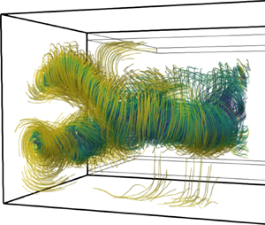
To study the effects of the superposition of thermal and forced convection, we conducted experiments in an RBC-like rectangular sample with added in- and outlet vents, see § 2.1. This corresponds to the trend of investigating flows with closer connections to engineering problems (Xia Reference Xia2013). As displayed in figure 1(c), Kühn et al. (Reference Kühn, Ehrenfried, Bosbach and Wagner2012) report that this flow arranges itself in a zigzag-like structure. This means the single longitudinal convection roll (figure 1b), which exists in pure forced convection (Schmeling et al. Reference Schmeling, Westhoff, Kühn, Bosbach and Wagner2011), realigns in the shape of multiple diagonal segments or LSCs caused by the additional buoyancy forces. Furthermore, these LSCs can be observed as counter-rotating circulations in a vertical longitudinal section (Westhoff et al. Reference Westhoff, Bosbach, Schmeling and Wagner2010). They then have a similar appearance as the multiple LSCs of pure RBC in the same geometry, see figure 1(a) (Kaczorowski & Wagner Reference Kaczorowski and Wagner2009; Podvin & Sergent Reference Podvin and Sergent2012).
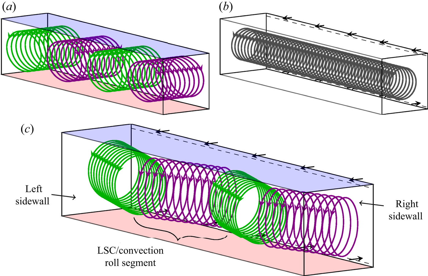
Figure 1. Comparison of the conceptual flow structures of pure RBC (a), pure forced convection (b) and mixed convection (c) in a rectangular sample. The flow structures are visualised by generic streamlines (green, purple, black). The respective forcing is indicated by the heated (red) and cooled (blue) faces (a,c) as well as by flow arrows at the in- and outlet at the rear wall (b,c). For mixed convection (c), the flow structure aligns in the shape of a zigzag with multiple convection roll segments or LSCs according to Kühn et al. (Reference Kühn, Ehrenfried, Bosbach and Wagner2012). The displayed formation comprises four LSCs spanning between the sidewalls.
An analogy to this break up of a longitudinal roll can be found in turbulent mixed convection channel flow (Pirozzoli et al. Reference Pirozzoli, Bernardini, Verzicco and Orlandi2017; Blass et al. Reference Blass, Zhu, Verzicco, Lohse and Stevens2020). There, the heat transporting convection rolls align longitudinally to the main flow direction but start to meander at  $Ri\approx 10^0$. This observed instability is similar to the wavy instability, which Clever & Busse (Reference Clever and Busse1991) explain and Pabiou, Mergui & Bénard (Reference Pabiou, Mergui and Bénard2005) prove for laminar flows by means of experiments.
However, regarding turbulent mixed convection in the here considered cuboidal convection sample, Westhoff et al. (Reference Westhoff, Bosbach, Schmeling and Wagner2010) measured a low frequency oscillation of the fluid temperature at the outlet of the sample and also show that the roll core positions in different cross-sections vary over time. In the following, Schmeling, Bosbach & Wagner (Reference Schmeling, Bosbach and Wagner2013) identify different types of flow instabilities by means of temperature measurements using a sensor array positioned in the sample. The resulting temperature fields exhibit hot and cold spots representing sections of the up- and down-welling flow of the zigzag roll structure. Based on the temperature time series of single probes, two types of dynamical behaviour are distinguished: continuous temperature oscillations ( $\mathcal {C}$) and spontaneous ( $\mathcal {S}$) events occurring stochastically on longer time scales. For both types, the temperature signals indicate that the hot and cold spots move through the sample along the longitudinal direction. Projecting these motions on the zigzag roll structure implies a travelling of the roll segments. Accordingly, roll segments emerge and break down at the opposing sidewalls in this model conception. A specific event of type $\mathcal {S}$ was observed by Westhoff (Reference Westhoff2012, pp. 54–70) performing long-time two-dimensional, two-component PIV measurements in the central longitudinal section of the sample. The subsequent POD shows changes between four-roll and three-roll states, respectively, associated with the first and second modes of the decomposition. These findings are in agreement with the proposed process of Schmeling et al. (Reference Schmeling, Bosbach and Wagner2013).
Since the causes of both dynamical behaviours have not yet been identified in existing research, the understanding of these processes will also benefit from the intended transfer of RBC model concepts. Consequently, we conducted tomographic PIV measurements with simultaneous temperature measurements of both  $\mathcal {C}$- and $\mathcal {S}$-type events to contribute to the understanding of the process. The results were examined with respect to parallels to instabilities found in RBC. In particular, PODs were conducted on the basis of the velocity fields obtained during the reconfiguration events. This analysis allows us to discuss the influence of the resulting coherent structures in the style of the approach of Podvin & Sergent (Reference Podvin and Sergent2015).
2. Experimental set-up
2.1. Mixed convection sample
We investigated the flow in an enclosure with the dimensions  $L=2500\ \mathrm {mm}$ and $H=W=500\ \mathrm {mm}$ defining the aspect ratios $\varGamma _{XY}=5$ and $\varGamma _{YZ}=1$. A sketch of the sample is presented in figure 2 which also comprises the experimental instrumentation, see § 2.2. The temperature boundary conditions of the sample were defined by a blackened aluminium bottom plate ( $T_{{HP}}$) heated by tempered water and a top plate ( $T_{{CP}}$) of the same material passively cooled to room temperature. The lateral faces were double-walled by 10 mm thick polycarbonate to minimise heat exchange with the surroundings while allowing optical access. A 25 mm high inlet vent (A) was positioned along the top edge of the rear wall, and a 15 mm high outlet (B) at the bottom edge. This set-up allowed us to study mixed convection, as both buoyancy and inertial forces can be induced in the fluid sample. The direction of the forced flow is indicated by the arrows inside the ducts in figure 2.

Figure 2. (a) Mixed convection sample with the used measurement set-up. A - inlet vent. B - outlet vent. C - LED light source. D - PIV camera system. The resulting PIV domain is highlighted in green. The positions of the temperature sensors near the rear wall are marked by black dots. (b) Photograph of the mixed convection sample.
The prevalent flow state in the sample depends on the dimensionless parameters representing the thermal forcing  $Ra=g \,\beta \, {\rm \Delta} T\, H^3/(\nu\, \alpha)$, the inertial\query{Q10} forcing $Re ={v_{in}\, H}/{\nu }$ and the relation between momentum and heat transport, namely the Prandtl number $Pr ={\nu }/{\alpha }$. With air as working fluid, $Pr \approx 0.7$ was assumed to stay constant for the investigated parameter range. The other dimensionless parameters were varied by changing the temperature difference between the top and bottom plates ${\rm \Delta} T=T_{{HP}}-T_{{CP}}$ and the mean inflow velocity $v_{in}$. In particular, we adjusted ${\rm \Delta} T$ through $T_{{HP}}$ as the top plate was passively cooled. Moreover, the volume flow rate $\dot {V}$ of the air entering the sample via the opening of the inlet $A_{in}$ determines the mean inflow velocity $v_{in} = {\dot {V}}/{A_{in}}$. Except for the sample height $H$ and gravitational acceleration $g$, all other quantities determining the dimensionless numbers were material parameters: they comprise the thermal expansion coefficient $\beta$, the kinematic viscosity $\nu$ and the thermal diffusivity $\alpha$.
In order to generate a sufficiently developed velocity profile at the inlet, the inlet channel had a length equalling 30 times its height. The first  $100\ \mathrm {mm}$ were equipped with aluminium honeycomb material with an inner diameter of $3\ \mathrm {mm}$ in order to homogenise the flow. Further details of the sample were described by Kühn et al. (Reference Kühn, Ehrenfried, Bosbach and Wagner2011) regarding the realisation of the apparatus, and by Schmeling et al. (Reference Schmeling, Bosbach and Wagner2013) regarding the characterisation of the experiment's boundary conditions.
Schmeling et al. (Reference Schmeling, Bosbach and Wagner2013) also presented a set of parameter configurations which allows estimations in terms of the parameter spaces in which  $\mathcal {C}$- and $\mathcal {S}$-type reconfiguration events can be expected. Therefore, the Richardson number ${Ri} = {{Ra}}/{{Pr}\cdot {Re}^2}$, which defines the relation of thermal to forced convection, is used as main distinction between the event types.
The  $Re$–
$Re$– $Ri$ parameter space based on Schmeling et al. (Reference Schmeling, Bosbach and Wagner2013) is composed of areas with stable states (blue) as well as of states exhibiting reconfigurations of $\mathcal {S}$- (red) and $\mathcal {C}$-type (green), see figure 3. In order to generate different types of reconfiguration events, we applied the parameter sets $Ri_{\mathcal {S}}=3.7, Ra_{\mathcal {S}}=1.4\times 10^8, Re _{\mathcal {S}}=0.7\times 10^4$ and $Ri_{\mathcal {C}}=1.5, Ra_{\mathcal {C}}=1.6\times 10^8, Re _{\mathcal {C}}=1.2\times 10^4$, which lie in the respective ranges.
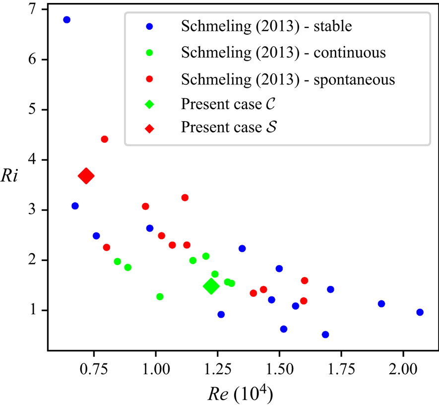
Figure 3. Parameter space with the classification determined by Schmeling et al. (Reference Schmeling, Bosbach and Wagner2013): stable states as well as continuous and spontaneous reconfigurations are indicated by blue, green and red dots, respectively. Additionally, the cases studied in this work are marked by diamonds: the red diamond marks case  $\mathcal {S}$ ( $Ri=3.7, Ra=1.4 \times 10^8, Re =0.7\times 10^4$) and the green one marks case $\mathcal {C}$ ( $Ri=1.5, Ra=1.6\times 10^8, Re =1.2\times 10^4$).
It should be noted that the Archimedes number  $Ar$ was used as synonym for $Ri$ in the publication of Schmeling et al. (Reference Schmeling, Bosbach and Wagner2013).
2.2. Measurement arrangement
The measurement system was composed of a tomographic PIV set-up intended to investigate the evolution of flow structures and a temperature sensor array allowing a fast classification of the present flow state.
While Schmeling et al. (Reference Schmeling, Bosbach and Wagner2013) used a temperature sensor array spread throughout the bulk sample for their investigations, we opted for a rear wall-bound arrangement to ensure optical accessibility of the PIV domain. Furthermore, wall-bound temperature measurements are a standard procedure for similar investigations in RBC (Brown & Ahlers Reference Brown and Ahlers2006; Funfschilling et al. Reference Funfschilling, Brown and Ahlers2008; Bai et al. Reference Bai, Ji and Brown2016). Typically, the probes are circumferentially arranged at different heights. However, we reduced the sensor array exclusively to one line at the rear wall of the sample. This arrangement still provided sufficient information about the flow state as the forced flow fixes the up-welling fluid section to the rear wall for the investigated parameter range. The array comprised 17 Pt100 resistive temperature sensors of precision class AA (IEC 2008). They were positioned at a height of  ${H}/{4}$ and in a distance of ${W}/{50}$ to the rear wall, in accordance with Wessels et al. (Reference Wessels, Schmeling, Bosbach and Wagner2019). Their arrangement is indicated by the black dots in figure 2. The sensor resistances were acquired by a scanning multimeter resulting in a measurement period of ${\rm \Delta} t \approx 8.7\ \mathrm {s}$ for each single sensor. This frequency is of the order of the turnover frequency of the main convection roll. As the reconfiguration events occur on time scales at least one order of magnitude larger, this acquisition frequency was sufficient.
The measured temperature distribution is physically related to the global flow structure as  $Y$-displacements of the convection roll are accompanied by changes in the temperature field. Therefore, changes of the rear-wall temperature distribution correspond to variations of the longitudinal distribution of LSCs (Niehaus et al. Reference Niehaus, Mommert, Schiepel, Schmeling, Wagner, Dillmann, Heller, Krämer, Wagner, Tropea and Jakirlić2020).
Due to this interdependence, the temperature measurements also indicate the beginning of a flow reconfiguration event. Thus, we used them to trigger the PIV when a spontaneous reconfiguration occurred. This was necessary as the seeding precipitation during PIV would have affected the boundary conditions for longer ring buffer-based measurements. Details on the implementation of the trigger condition are described by Mommert et al. (Reference Mommert, Schiepel, Schmeling and Wagner2019).
In terms of the tomographic PIV set-up, we decided to measure the flow in the vicinity of the left sidewall in order to capture the expected structure formation process, which is part of the reconfiguration process described by Schmeling et al. (Reference Schmeling, Bosbach and Wagner2013).
The corresponding PIV set-up is presented in figure 2. It shows the arrangement of the LED illumination (C), the camera system (D) and the measurement domain highlighted in green. To achieve particle images with sufficient contrast for PIV in a domain of this size, we chose the approach of LED-illuminated helium-filled soap bubbles similar to Kühn et al. (Reference Kühn, Ehrenfried, Bosbach and Wagner2012). Further information on the PIV system and its configuration for the measured cases can be found in table 1.
Table 1. Recording parameters for tomographic PIV.
To ensure the required projection accuracy for the tomographic reconstruction of the acquired frames, we applied a volume self-calibration (Wieneke Reference Wieneke2008) for each measured case in addition to the standard procedure of defining a mapping polynomial by capturing targets with known positions. Subsequently, tomographic reconstructions were performed using the simultaneous multiplicative algebraic reconstruction technique (Mishra, Muralidhar & Munshi Reference Mishra, Muralidhar and Munshi1999). The velocity vectors were then determined by a three-dimensional cross-correlations. Except for minor changes, the algorithm of Kühn et al. (Reference Kühn, Ehrenfried, Bosbach and Wagner2011) was used for these procedures. Outlier velocity vectors were replaced after identifying them in two steps: First, all vectors with an unphysically high magnitude  $\|\boldsymbol {u}\| \geq 1.6 v_{in}$ or low PIV correlation coefficient $r_{3D}<0.2$ were marked. Second, further vectors of the remaining unmarked vectors were marked by means of the universal outlier detection (Westerweel & Scarano Reference Westerweel and Scarano2005). Afterwards, all marked vectors were replaced by an interpolation between valid neighbouring vectors as methods like POD require gapless data. The number of outliers replaced in this way amounted to approximately 10 % with the outliers being randomly distributed in the measurement volume.
3. Proper orthogonal decomposition
The characteristics of the different reconfiguration types were investigated by performing a POD analysis in order to determine the flow's coherent structures and their manifestation over the course of time in § 4.
For the POD, each velocity vector field is reshaped into a single-state column vector  $\boldsymbol {u}_{t}=[u_{X,(1,1,1)},u_{Y,(1,1,1)},u_{Z,(1,1,1)},\ldots ,u_{Z,(I,J,K)}]$. In this context, $I$,
$I$, $J$ and $K$ are the number of grid points along the coordinate axes of the PIV domain.
Subsequently, the method of snapshots (Sirovich Reference Sirovich1987) is applied to achieve the decomposition of these vectors into  $k$ hierarchical modes $\boldsymbol {\phi }_k$ and the respective time coefficients $a_{k,t}$ as shown in (3.1)
 \begin{equation} \boldsymbol{u}_{t} = \sum_k a_{k,t}\,\boldsymbol{\phi}_k. \end{equation}
 Therefore, the series of  $N$ discrete measurements in form of $\boldsymbol {u}_{t}$ are merged into the state matrix ${\boldsymbol{\mathsf{U}}}$
 \begin{equation} {\boldsymbol{\mathsf{U}}} = \left[ \begin{array}{cccc} | & | & & | \\ \boldsymbol{u}_1 & \boldsymbol{u}_2 & \ldots & \boldsymbol{u}_N \\ | & | & & | \end{array}\right].\end{equation}
 Next, the auto-correlation matrix  ${\boldsymbol{\mathsf{C}}}$ is calculated
 \begin{equation} {\boldsymbol{\mathsf{C}}} = {\boldsymbol{\mathsf{U}}}^\top {\boldsymbol{\mathsf{U}}} . \end{equation}
 Solving the eigenvalue problem of (3.4) yields time coefficient vectors  $\boldsymbol {a}_k=[a_{k,1},a_{k,2},\ldots ,a_{k,N}]$ and mode-related eigenvalues $\lambda _k$
 \begin{equation} {\boldsymbol{\mathsf{C}}} \boldsymbol{a}_k = \lambda_k \boldsymbol{a}_k. \end{equation}
 As each element of the auto-correlation matrix  ${\boldsymbol{\mathsf{C}}}$ is a product of two velocity components, the eigenvalues $\lambda _k$ represent a measure of the kinetic energy contained in a mode. Spatial representations $\boldsymbol {\phi }_k$ of the latter can then be computed by
 \begin{equation} \boldsymbol{\phi}_k = {\boldsymbol{\mathsf{U}}} \boldsymbol{a}_k. \end{equation}
For the interpretation of the modes, it is important to consider that translatory moving coherent structures are not extracted into single modes by the POD method. Instead, this method distributes the moving structure to a set of modes, similar to a Fourier decomposition, in order to reproduce the movements (Brunton & Kutz Reference Brunton and Kutz2019, pp. 396–397). Such a Fourier-like representation is related to a slow decay of the eigenvalues. As Schmeling et al. (Reference Schmeling, Bosbach and Wagner2013) conjecture a translation of flow structures, the PODs have to be interpreted with particular care with regard to this issue.
Furthermore, it should be noted that the present PODs were based on the uncentred state matrices  ${\boldsymbol{\mathsf{U}}}$. This is of particular interest, as the first mode of an uncentred POD can be similar to the averaged field. That way, the POD also quantifies the energy contained in that structure.
4. Results and discussion
4.1. Rear-wall temperature distribution
The first part of the analysis focuses on the temperature data to establish a relation to previous studies and to gain first information about the time development of the reconfiguration processes including their consistency.
In order to identify the LSCs based on local temperatures, the evolution of the spatial interpolation between the rear-wall sensors is displayed in figure 4 for the considered cases  $\mathcal {S}$ and $\mathcal {C}$. It displays the respective time-averaged temperature distributions on the left side: while the two hot spots ( ${L}/{4},{3L}/{4}$) of the stable periods become visible for case $\mathcal {S}$, the distribution of case $\mathcal {C}$ shows no clear structures as this case did not exhibit stable periods.
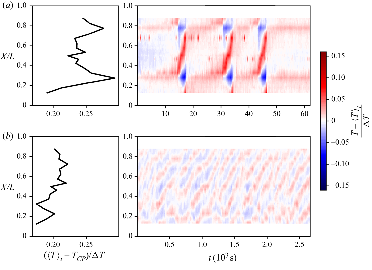
Figure 4. Time-averaged temperature distributions for the rear-wall sensor array (left) and the time evolutions of the deviations from the mean value (right) shown for both cases  $\mathcal {S}$ (a) and $\mathcal {C}$ (b).
The evolutions of the associated temperature deviations on the right of figure 4 reveal a number of hot spots (HS) mainly moving from the left to the right  $X$-positions for both cases. During the reconfiguration events of case $\mathcal {S}$, the deviations become more intense, as the structure of the stable periods is already imprinted on its mean distribution.
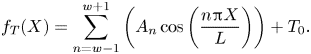
The main distinctive features of the cases are the time scales of the hot spots’ dynamics and the number of implied LSCs. To quantify the latter, we consider the following: each hot spot is associated with up-welling warm fluid, whereas the compensating colder flow regions are located on the hot spot's sides and expressed as cold patches in figure 4. For an initial guess, the wavenumber  $w$, here defined by the number of LSCs, was calculated by the distances ${\rm \Delta} X$ between a hot and a cold spot (CS) or two hot or cold spots:
 \begin{equation} w \approx \frac{L}{{\rm \Delta} X_{{HS-CS}}} \approx \frac{2L}{{\rm \Delta} X_{{HS-HS}}} \approx \frac{2L}{{\rm \Delta} X_{{CS-CS}}}. \end{equation}
 On this basis, we estimated  $w_{\mathcal {S}}=4$ and $w_{\mathcal {C}}=8$ for the respective cases. These numbers correspond to the findings of Westhoff (Reference Westhoff2012, pp. 54–59), who also found these two wavenumbers associated with high and low $Ri$ in a study of turbulent mixed convection cases with cases with similar $Ra$.
$Ra$.
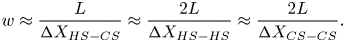
In order to gain temporal information on this matter, the number of LSCs was determined over the course of time by applying a cosine-based curve fit (4.2) to the instantaneous temperature distributions  $T_t(X)$. The fit parameters were determined by minimising the sum the residuals’ squares with Newton's method. As the temporal resolution was sufficient to continuously resolve transformation processes, the established fit parameters of the previous instant were used as starting conditions for the succeeding time step. Since the reconfiguration process is characterised by decaying and emerging LSCs (Schmeling et al. Reference Schmeling, Bosbach and Wagner2013), we focused on the cosine summands next to the suggested wavenumbers $w_{\mathcal {S}}=4$ and $w_{\mathcal {C}}=8$. Besides the number of LSCs, further information about the states is contained in the sign of $A_n$. Thereby, a positive sign corresponds to a hot spot at the left sidewall.
 \begin{equation} f_T(X) = \sum_{n=w-1}^{w+1}\left( A_n \cos\left(\frac{n \pi X}{L}\right)\right)+T_0. \end{equation}
 For both cases, the amplitudes  $A_n$ are plotted in figures 5 and 6, respectively. Regarding case $\mathcal {S}$, the absolute amplitudes show that a reconfiguration event consists of multiple changes between 4 and 3 LSC states, while $|A_5|$ never dominates. However, during the multiple hour long periods of stability, $|A_3|$ and $|A_5|$ are steadily rising. Similar rises can be observed for $|A_3|$ during the short 4 LSC periods of the reconfiguration events.
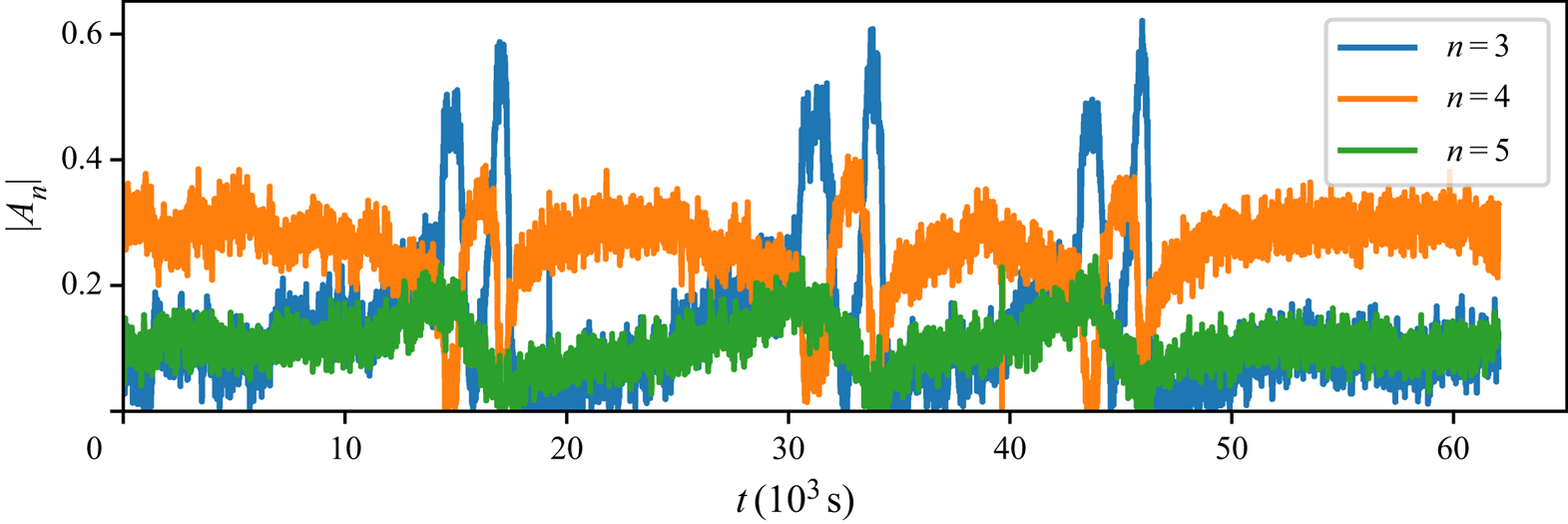
Figure 5. Temporal development of the absolute values of the cosine fit amplitudes  $|A_n|$ implying the number of LSCs in the sample for case $\mathcal {S}$.
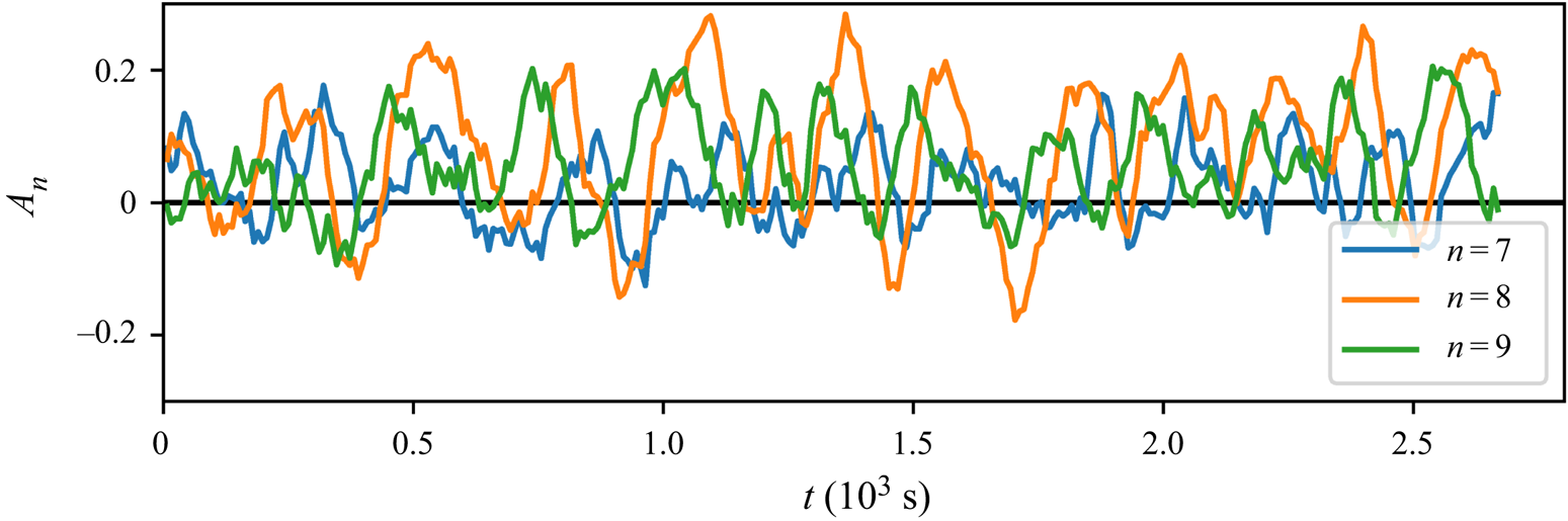
Figure 6. Temporal development of the cosine fit amplitudes  $A_n$ implying the number of LSCs in the sample for case $\mathcal {C}$.
This shows that case  $\mathcal {S}$ is characterised by a continuous reconfiguration process although it exhibits distinct events. The existence of a quasi-stable period between the events indicates that there is a preferred flow state with four LSCs.
Figure 7 allows us to describe the process in more detail as it depicts the phase space of the signed amplitudes  $A_n$. It visualises the quasi-stable periods of the preferred state as an accumulation of data points representing a 4 LSC state with $A_4<0$. This means that the cold areas appear at the sides of the sample for most of the time, which was also found to be the stable configuration for a wide $Ra$-range in numerical simulations of RBC (Kaczorowski & Wagner Reference Kaczorowski and Wagner2009).
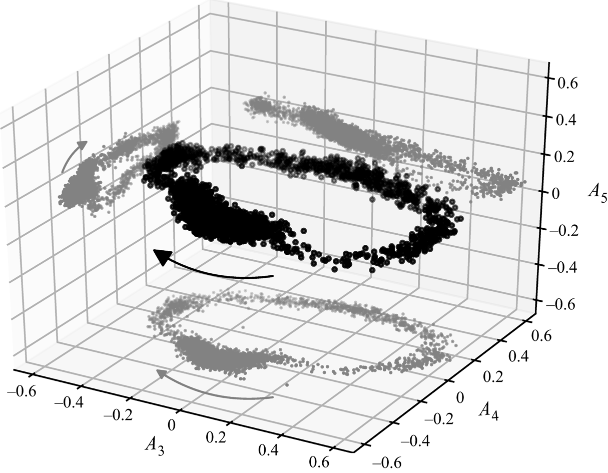
Figure 7. Phase space of the fit amplitudes  $A_n$ of case $\mathcal {S}$ allowing us to determine the exact orientation by the means of the amplitudes’ sign.
As the depiction covers three events which cannot be distinguished, it shows that they proceed as a consistent process: the preferred 4 LSC state is followed by a 3 LSC state with a cold left side ( $A_3<0$). The flow then passes through a 4 LSC state with warm sides before the circle is closed by traversing a 3 LSC state with a warm left side. Such a switching between states with different retention times was also observed by Xie, Ding & Xia (Reference Xie, Ding and Xia2018) in an annular RBC sample. In contrast to their study, the two main states in the present investigation exhibit the same wavenumber and only their transition is predominated by a state of a lower wavenumber.
During the whole process,  $A_5$ plays only a minor role. This is in good agreement with the observations of Schmeling et al. (Reference Schmeling, Bosbach and Wagner2013), which describe the same cycle process with an LSC decay on the right side followed by the formation of a new LSC on the left side. Regarding the origin of these events, the slow rise of $|A_3|$ and $|A_5|$ during the quasi-stable phase also corresponds to the idea of a heat or momentum accumulation mechanism. That could further mean that the distinct spontaneous events equal the passing of an accumulation threshold accompanied by the release of the earlier accumulations similar to Sugiyama et al. (Reference Sugiyama, Ni, Stevens, Chan, Zhou, Xi, Sun, Grossmann, Xia and Lohse2010) or Wang et al. (Reference Wang, Lai, Song and Tong2018).
Regarding case  $\mathcal {C}$, the $A_n$ evolution shown in figure 6 reflects the continuous dynamics with a mean period of $t_{\mathcal {C}}\approx 215\ \mathrm {s}$. Our initial wavenumber guess is confirmed as the coefficient $A_8$ displays the highest amplitudes. Therefore, we define 8 LSCs as the underlying baseline for this case and use $A_8$ as an indicator for its dynamics. In contrast to case $\mathcal {S}$, the maximum amplitudes of $A_n$ are only half as large. This means that random turbulent fluctuations have a stronger influence and the reconfiguration process appears more chaotic. However, the following systematics are revealed: the intervals of sign change with positive gradient of $A_8$ display a positive $A_9$ as prevalent amplitude parameter. During a change of sign with negative gradient of $A_8$, a positive $A_7$ is prevalent.
This can be interpreted as follows: an 8 LSC state with cold sides transforms into an 8 LSC state with warm sides via the generation of a new counter-rotating LSC on the left side followed by the decay of the rightmost LSC. During the opposite transformation, the decay on the right side takes place first and is succeeded by the formation of a new LSC on the left side. Further, the observations also reveal a bias of case  $\mathcal {C}$ towards positive values of $A_n$, while for case $\mathcal {S}$ the differently signed extents of $A_3$ and $A_4$ were almost symmetric but varied in duration. The fact that this manifestation of the bias does not create quasi-stable states indicates that these reconfigurations are driven by different forces. Hence, the share of forced convection remains as the main driver for the reconfigurations case $\mathcal {C}$. This idea is followed up by the analyses of § 4.3.
Figure 8 also confirms the consistency of this case as a prevalent orbit exists in the phase space of case  $\mathcal {C}$. In contrast to case $\mathcal {S}$, the orbit is tilted inside the three-dimensional (3-D) phase space, as both, $A_7$ and $A_9$, play an important role.
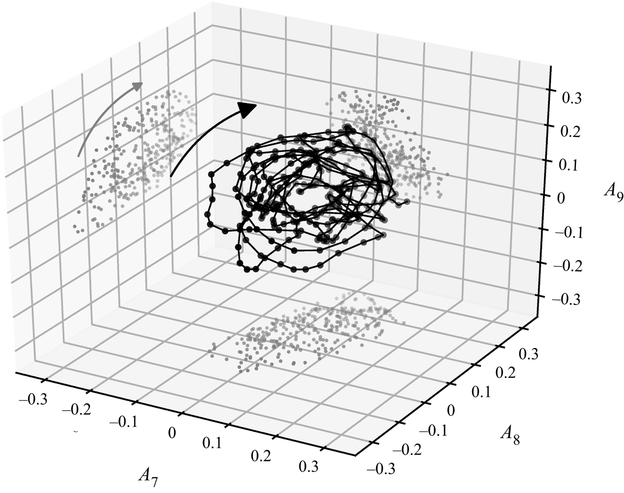
Figure 8. Phase space of the cosine fit amplitudes  $A_n$ for case $\mathcal {C}$. The displayed dots are moving averages of $A_n$ over 3 data points.
Despite possible differences regarding the driving forces, the findings of the temperature measurements indicate that the reconfiguration mechanisms of both cases are based on the translation of flow structures in the sample accompanied by the generation and decay of LSCs at the sidewalls. This result corresponds to the conclusions drawn by Schmeling et al. (Reference Schmeling, Bosbach and Wagner2013). To test this model concept, the results of 3-D PIV measurements performed during the presented time series are addressed in the next sections.
4.2. Velocity fields of spontaneous events
For assessing flow field information of an event of type  $\mathcal {S}$, we used a temperature-based trigger, see § 2.2. Especially, a condition checking for a change in the relation of two local temperatures between the previous ( $t-{\rm \Delta} t$) and latest (
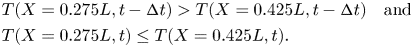
 $t$) measurements was found to be an indicator for the onset of an event in preliminary tests (Mommert et al. Reference Mommert, Schiepel, Schmeling and Wagner2019), see (4.3a,b). Its instant of occurrence is also marked by a circle in figure 9(a), which depicts the evolution of the respective temperature signals. Additionally, the colour-coded background indicates periods of $|A_3|$ or $|A_4|$ dominance based on the cosine fits.
 \begin{align} T(X&=0.275 L, t-{\rm \Delta} t) > T(X=0.425 L, t-{\rm \Delta} t) \quad \mathrm{and} \\ T(X&=0.275 L, t) \leq T(X=0.425 L, t). \end{align}
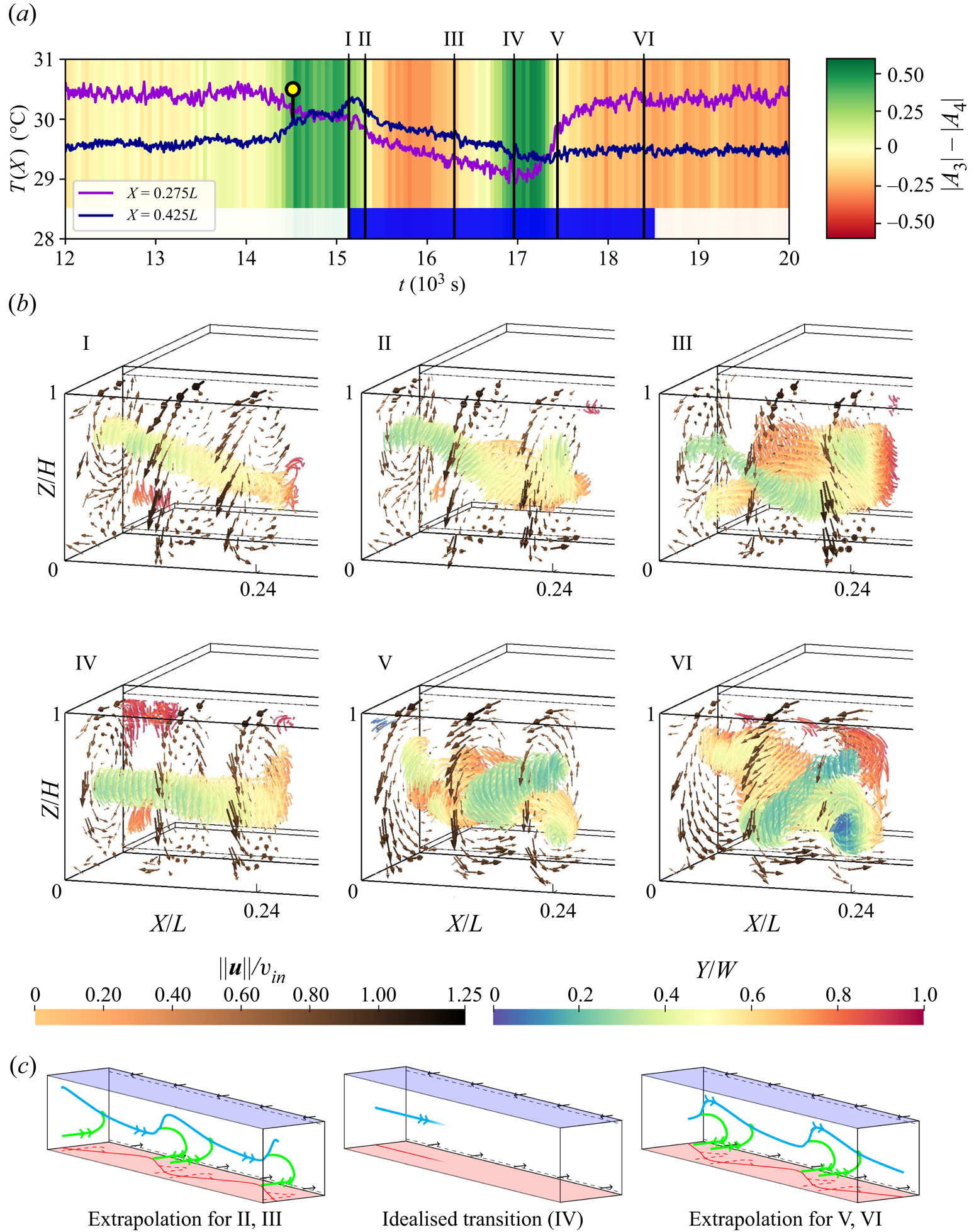
Figure 9. (a) Temperature time series recorded by selected sensors over the course of a reconfiguration event. The interval for which velocity fields were measured is marked by a blue bar. (b) Velocity fields for 6 points in time, which are indicated in the temperature series. The fields are represented by vectors in 3 cross-sections and streamlines in areas of  ${\|\boldsymbol {u}\|}/{v_{in}}<0.2$ reflecting the convection roll core. The displayed fields are short-time averaged over 9 frames. Supplementary movie 1, available at https://doi.org/10.1017/jfm.2020.705, shows the complete time series. (c) Sketches of the extrapolated or idealised flow structures. The main convection roll and the secondary branch are marked in blue and green, respectively. They are projected onto the bottom plate in red.
Limited by the delay for achieving a sufficiently high seeding density, we acquired flow data for the time span marked by a blue bar in figure 9(a), which covers approximately 75 % of the event. Exemplary flow fields of this time span are presented in figure 9(b). They comprise velocity vectors in three cross-sections and streamlines in regions of relatively low velocities ( ${\|\boldsymbol {u}\|}/{v_{in}}<0.2$) to visualise the convection roll structure in the domain.
Regarding the temperature analysis, the first observed state (I) represents the beginning of the transition from a 3 LSC configuration with prevalent cold temperatures at the left sidewall to four LSCs with a ‘warm sidewall’. At this instant, the streamlines reflect a single convection roll core with a diagonal alignment characterised by a displacement towards the front and top on the left side and rear and bottom on the right side. We assign this instant already to the onset of a 4 LSC state, as instants II and III display an intensified version of this alignment of the main roll core. At the same time, first traces of the formation of a secondary structure can be observed for instant II: at  $X \approx L/8$, another roll core branches out on the rear side of the main roll and extends to the left sidewall where it curves towards a $Y$-parallel alignment. This formation prevails throughout the dominance of $|A_4|$ as velocity field III represents a similar formation.
At time instant IV, the onset of the  $|A_3|$-dominant interval, the secondary structure vanishes and the diagonal displacement of the main roll from its central location is reduced. Thus, it can be considered as central and straight. With $|A_4|$ becoming dominant again at instant V, the main roll realigns with the inverse diagonal (left rear to upper right front) which also entails a secondary roll branch. For this alignment, the secondary structure branches also from the rear side of the main roll at $X \approx L/8$ and stretches to $X \approx L/4$ corresponding to the hot spot location at the rear wall. There, it aligns parallel to the $Y$-axis. Velocity field VI shows that this branch alignment is prevalent for the 4 LSC configuration observed during the remainder of the measurement period.
Especially, the occurrence of a secondary roll branch raises further questions with regard to possible links to corner roll-driven reversals in RBC; see Sugiyama et al. (Reference Sugiyama, Ni, Stevens, Chan, Zhou, Xi, Sun, Grossmann, Xia and Lohse2010) and Soucasse et al. (Reference Soucasse, Podvin, Rivière and Soufiani2019). For a stable mixed convection case, Kühn et al. (Reference Kühn, Ehrenfried, Bosbach and Wagner2012) also found  $Y$-parallel vortical structures, which occurred in pairs and were otherwise similar to the structure of the secondary branches. Therefore, we extrapolate that a mirrored secondary branch outside the PIV domain exists for fields like V or VI, see figure 9(c). Regarding their dynamic behaviour, we observed the decay of these branches at the onset of the reconfiguration rather than a growth. This rules out a reversal process analogous to RBC in quasi two-dimensional samples.
In the following our observations will be summarised and evaluated. In terms of the temperature analysis, we expected the following behaviour of the main convection roll: during  $|A_3|$-dominance, the diagonal segments stretch to fill the space along the $X$-axis. Under this assumption, the secondary branches persist and move corresponding to the hot spots over the course of a reconfiguration; compare with figure 4. However, we found that the flow structures occurring in the monitored part of the sample during $|A_3|$-dominance reflect a transition state without strong diagonal displacements or secondary roll branches; see instant IV. While a translational propagation of the secondary structures is plausible for more $X$-central regions of the sample, our observations contradict the translational model regarding the dynamics of the leftmost LSC. Rather, the motion of this segment of the main convection roll is described by the switch of orientation of the observed roll segment around a pivot at $X \approx L/8$, which we will refer to as switching. This raises the question why figure 4 displays a translating hot spot in the region overlapping the PIV domain, where no secondary structure was observed during the transition (see figure 9c).
The reason for these observations is that the position of the temperature sensor array leads to the acquisition of temperature footprints related to local structures occurring during the reconfiguration events. These structures are plumes which originate from the front bottom edge vortex of the sample. Figure 10 shows the position of the edge vortex in relation to the main convection roll and its secondary roll branch. In order to describe the mechanism responsible for a reconfiguration event, the longitudinal velocity component in the region of the edge vortex is depicted in figure 10(b). Similarly, figure 10(c) shows the spanwise-averaged vertical velocity component in the control region drawn in a).
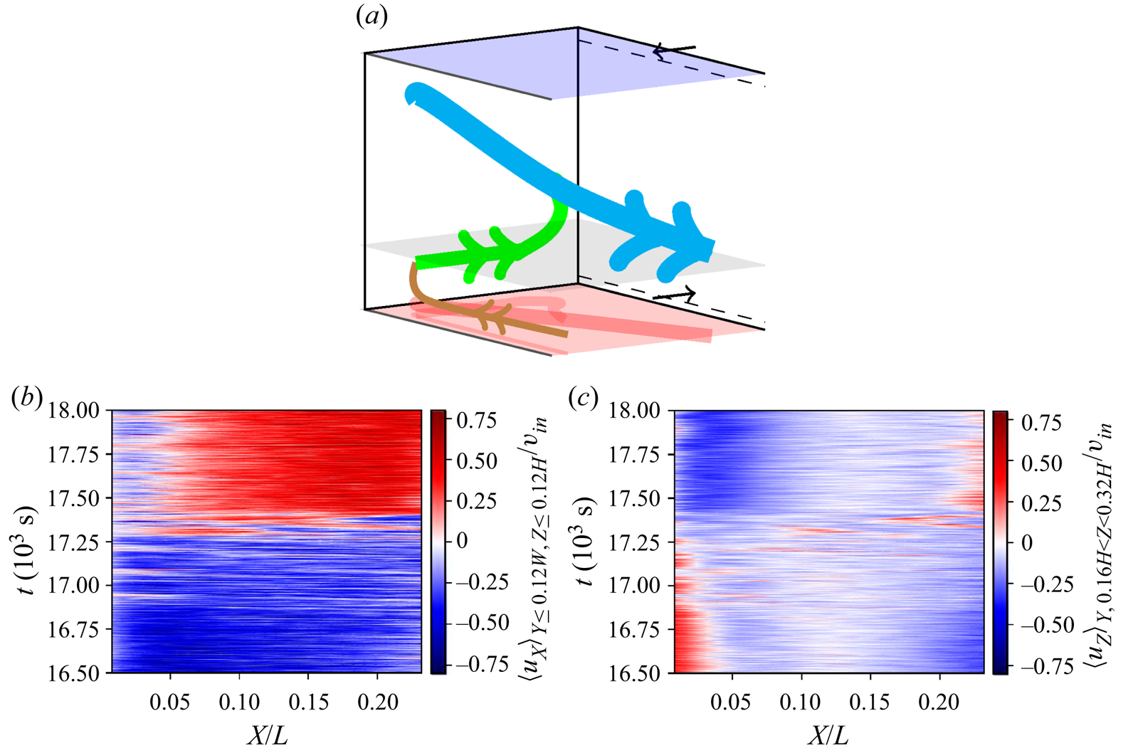
Figure 10. (a) Vortex system represented by angular momentum arrows in the PIV region of the sample. Blue: main convection roll. Green: secondary roll branch. Brown: front bottom edge vortex. Grey: control region for plume event analysis. (b)  $X$ velocity component averaged over the region of the edge vortex. (c) $Z$ velocity component averaged over the region of the control plane.
Regarding the longitudinal flow within the edge vortex, it is evident that this vortex transports fluids towards the secondary roll branch. However, this mechanism changes its direction, when the flow reconfigures itself ( $17.0\times 10^3\leq t\leq 17.5\times 10^3$). Similar to 2-D RBC (Sugiyama et al. Reference Sugiyama, Ni, Stevens, Chan, Zhou, Xi, Sun, Grossmann, Xia and Lohse2010), the edge vortex gathers heat from the bottom plate. Due to the small size of this circulation, the heat can hardly dissipate through the boundaries of the vortex. Therefore, the longitudinal convection within the vortex plays a major role when it comes to transporting the accumulated heat. Apparently, a reconfiguration occurs when this longitudinal transport is interrupted and switches its direction – most likely due to saturation effects. At the same time, the heat is not sufficiently removed from the edge vortex, which leads to multiple eruptions of plumes. The latter disturb the main roll and therefore promote its reorientation (see Huang & Xia Reference Huang and Xia2016). Evidence for these plume eruptions is provided by the averaged vertical velocity component in a control plane displayed in figure 10(c). It shows that footprints of these plumes occur when the longitudinal transport of the edge vortex switches direction. Therefore, the translation of hot spots observed in the temperature distributions of the rear wall is associated with events of local plume eruptions.
In the meantime, the macroscopic flow structure follows certain maximum and minimum principles: the two diagonal arrangements of the LSC represent potential minima. Regarding the changes between these states, the potential barrier for a switching appears lower than for a translation, as the latter would require the generation of a very narrow diagonal convection roll segment at the sidewall.
In order to gain insight into the macroscopic processes behind the switching of this roll segment, we investigated the underlying coherent structures. Hence, a POD was conducted with the instantaneous velocity fields. Applying the approach of Podvin & Sergent (Reference Podvin and Sergent2015), representations of the structure of the most prevalent modes and the respective eigenvalue distribution are presented in figure 11 for this case.
Figure 11. Eigenvalue distribution for the POD of case  $\mathcal {S}$ (a) and the four most prevalent modes normalised by the square root of the respective eigenvalue (b). Their structure is represented by the vectors of the highest magnitude. Supplementary movie 2 contains tracking shots of the displayed structures.
Most remarkably the first POD mode is represented by a vector field shaped like a longitudinal convection roll similar to the one of pure forced convection (Westhoff et al. Reference Westhoff, Bosbach, Schmeling and Wagner2010; Kühn et al. Reference Kühn, Ehrenfried, Bosbach and Wagner2012); see figure 11(b). Although the Richardson number  $Ri=3.7$ indicates that a buoyancy dominated flow exists, this forced convection mode acquires 60 % of the kinetic energy. However, it will be shown that the flow dynamics is mainly represented by the second mode, which we assign to the contribution of thermal convection. This is due to the fact that the large-scale circulation of the second mode is aligned in $Y$-direction. This agrees with the alignment obtained for pure thermal convection, i.e. RBC, in samples with the same aspect ratios (Kaczorowski & Wagner Reference Kaczorowski and Wagner2009; Podvin & Sergent Reference Podvin and Sergent2012). The fraction of the second mode's eigenvalue amounts to 11.5 %. With both $X$- and $Y$-angular momenta covered by the first two modes, these allow us to reconstruct the convection roll's diagonal alignment and rotation in the central $XY$-plane. Although only 2 % and 1 % of the overall energy is contained in the following modes, their influence on the reconfiguration process cannot be excluded: these modes also mark the transition from large-scale contributions to the coverage of localised structures. The third mode comprises not only a large-scale circulation aligned in $Z$-direction but also a strong contribution to an upward flow near the front left vertical edge of the sample. Mode 4 is even more localised, with a downward flow in the front part of the sample, which makes the strongest contribution at $X\approx 0.14L$. Regarding the considerations on PODs in terms of translating structures, it is certain that the present POD does not represent a translation-dominated process, since the eigenvalues would decline significantly slower in that case (Brunton & Kutz Reference Brunton and Kutz2019, pp. 396–397). Further, modes 3 and 4 do not display structures comparable to Fourier modes, that means multiple rolls with a $Y$-angular momentum. Instead, they show more localised and complex structures as the example of mode 4 shows. However, no further modes will be presented due to the advancing decline of their eigenvalues and therefore decreased contribution to the flow.
Another reason for this can be deduced from figure 12 displaying the temporal development of the modes: higher modes cover structures associated with small(er)-scale turbulence and increasing measurement noise which results in the time evolution becoming noisier and harder to interpret.
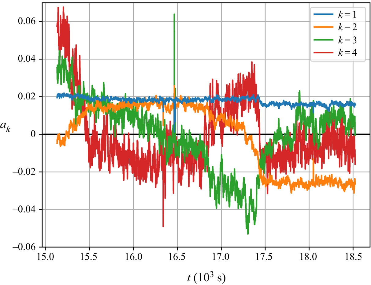
Figure 12. Time development coefficients for the first four POD modes as presented in figure 11.
However, the presented modes allow us to shed more light on the flow processes during a reconfiguration event: the first mode's coefficient remains constant until  $t\approx 17.5\times 10^3\ \mathrm {s}$, then it drops from $0.02$ to $0.016$. We explain this drop as an artefact of the incomplete reconfiguration process as input of the POD. It can also be retraced in an imperfection of the longitudinal convection roll visible at the left vertical edge of the vector plot $k=1$ in figure 11. However, since the change of this coefficient is small compared to the dynamic of the other coefficients, the reconfiguration is captured sufficiently by the POD.
The coefficient of mode 2 crosses zero at  $t\approx 15.2\times 10^3\ \mathrm {s}$ and rises to $0.02$ where it remains stable during the time span $15.75\times 10^3\ \mathrm {s}\leq t\leq 16.75\times 10^3\ \mathrm {s}$. Afterwards, it falls with increasing rates to a value of $-0.025$ and levels off for the remainder of the time series. As for the influence on the flow, the coefficient's changes of sign at ${t\approx 15.2\times 10^3\ \mathrm {s}}$ and ${t\approx 17.3\times 10^3\ \mathrm {s}}$ imply that the main thermally induced structure reverses twice during a reconfiguration event. Interpreting this in the context of super-positioned angular momenta, a reversing second mode reflects a change in the diagonal alignment of the main convection roll by rotation (see Soucasse et al. Reference Soucasse, Podvin, Rivière and Soufiani2019; Vasiliev et al. Reference Vasiliev, Frick, Kumar, Stepanov, Sukhanovskii and Verma2019).
This poses the following question: how do the buoyancy-induced coherent structures behave in comparison with the LSCs of RBC?
A similarity to the cessations observed in cylindrical RBC (Brown & Ahlers Reference Brown and Ahlers2006) is indicated by the two zero crossings in the time course of the coefficient of the second mode. These two zero crossings reflect that the main structure driven by the buoyancy force ceases to exist during reconfiguration events. The cessation process is, like other Poisson processes in cubic RBC (Bai et al. Reference Bai, Ji and Brown2016), based on the breaking of a potential barrier by turbulent fluctuations. However, taking the remaining modes 3 and 4 into account contradicts the explanation of random fluctuations as a cause for the reversals of the present case: in particular, the coefficients of mode 3 and 4 display increased absolute values during the sign changes of mode 2 and lower ones during the level intervals of mode 2. This means that momentum is transferred between the coherent structures of mode 2 and the two following modes. Thus, this exchange resembles a coordinated process rather than random fluctuations as it proceeds for both sign changes of mode 2.
Further investigation of mode 3 in figure 12, reveals that this mode approximates the change rate of mode 2. As mode 3 is associated with an angular momentum in the  $Z$-direction, it might represent a azimuthal motion which drives the reconfiguration (see Vasiliev et al. Reference Vasiliev, Frick, Kumar, Stepanov, Sukhanovskii and Verma2019). However, the consideration of the sign of $a_3$ yields an azimuthal flow contrary to the one expected from the evolution of the flow structure. That means the observed reconfigurations are not driven by azimuthal flow. Rather, the $Z$-oriented rotation of mode 3 adds another, vertical angular momentum component to the model describing the diagonally aligned convection roll with the first two modes. This way, mode 3 mainly represents an additional vertical tilt of the convection roll core. Tangible descriptions of its effect are given by the depiction of the reconstructed roll cores in figure 13: the addition of mode 3 allows the reconstruction of a stronger elevation of the roll core next to the sidewall for time step II. On the contrary, the correct central core position at time step IV is also achieved by including mode 3.
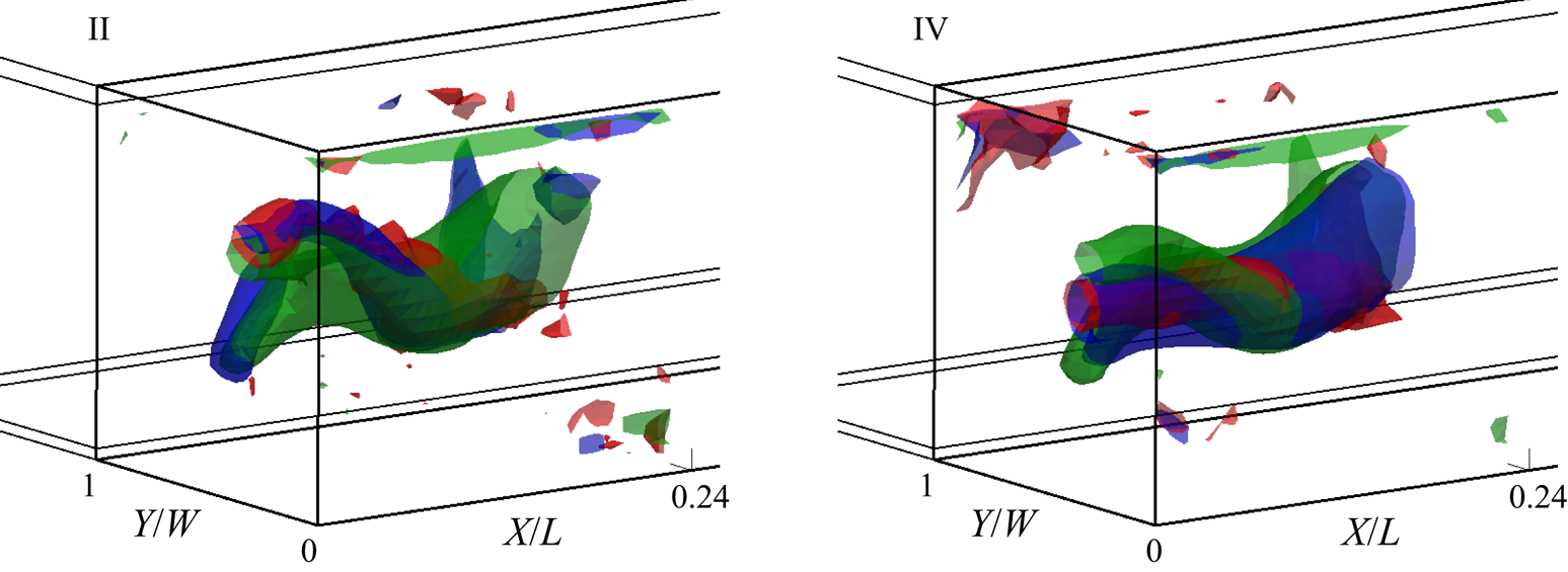
Figure 13. The  ${\|\boldsymbol {u}\|}={v_{in}}/8$ isosurfaces representing the convection roll core for the short-time average PIV fields (red) and the POD reconstructions with the modes $k\leq 2$ (green) and $k\leq 3$ (blue) for the times II and IV from figure 9(a). Tracking shots of these isosurface plots are part of supplementary movies 3 and 4.
Furthermore, the time coefficient of mode 3 falls constantly in the period  $15.75\times 10^3\ \mathrm {s}\leq t\leq 16.75\times 10^3\ \mathrm {s}$, in which the direct observation of the flow fields revealed no significant transition process. This again underlines the presence of a accumulation and release reversal mechanism (Wang et al. Reference Wang, Lai, Song and Tong2018). In detail, the kinetic energy accumulated in the coherent structures of mode 3 is released and transferred to mode 2 rather quickly after a critical level was reached ( $t\approx 17.4\times 10^3\ \mathrm {s}$).
Further indication for this kind of process is provided by mode 4: it keeps fluctuating around  $-0.01$ for most of the time but shows elevated values surpassing $0.03$ while the large-scale flow structure is being transformed. Spatially, this mode has the strongest contributions at $X\approx 0.14L$, see figure 11. Hence, we associate its flow structure with the ‘release’ which triggers the progression of the reconfiguration.
More information about the characteristics of the present reconfiguration event can be deduced from its progression in the phase space of the time coefficients of modes 2 and 3 displayed in figure 14. It shows, that approximately three quarters of the reconfiguration cycle are covered by the measurement, which is consistent with the temporal consideration of figure 9(a). The distribution of flow states in this phase plane further reveals an elliptical shape. While it is almost axisymmetric to  $a_3=0$, its extent in the $a_2$ direction is larger in the negative direction. This might be caused by parts of the secondary roll branch inherent to this mode. Another possible explanation is that negative $a_2$ values represent the flow state which is preferred in comparison with the reversed one.
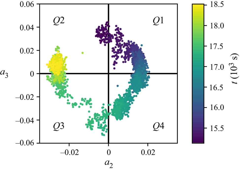
Figure 14. Phase space of the modes 2 and 3 during a reconfiguration event.
Besides that eccentricity, the point density reveals the rate at which the states change. This also indicates an accumulation and release process, as the state evolves slowly around  $a_3=0$ as well as in quadrant $Q4$ and rapidly in the quadrants $Q1$ and $Q3$.
$Q3$.
Projecting the progression of  $Q4$ onto $Q2$ yields point-symmetric change rates relative to the origin. This indicates that both diagonally aligned states of the main convection roll can be considered as meta-stable states with similar mechanisms depleting their stability.
To identify relations between the different dynamics of the temperature and velocity field, we conducted correlations of the cosine and POD coefficients, see figure 15. It reveals that the prevalence of the 4 LSC state ( $A_4$) strongly correlates with the respective coherent structure determined by the POD $\rho _{A_4a_2}=0.96$. During the events, both $A_3, A_5$ and $a_3, a_4$ become particularly active. However, only $a_3$ yields reasonable correlation coefficients for $\rho _{A_3a_3}$ and $\rho _{A_5a_3}$ with differing signs. However, these correlations may be coincidental, as the structure of mode 3 itself does not contain flow structures explaining rear-wall hot spots, whose positions would match the implied wavenumbers. As the cosine functions cover the complete sample, connecting features between the temperatures and the flow process represented by mode 3 might also exist outside the PIV domain. Regarding $a_4$, only low correlation values are registered. However, the ‘ $<$’-shape of the correlation plots indicates that there is a correlation with the absolute values of $|A_3|$ and $|A_4|$. That means this mode is associated with the transition period characterised by the hot spot movement. This also explains that, the mode's contribution is of the same sign for both directions of the reversal of mode 2.
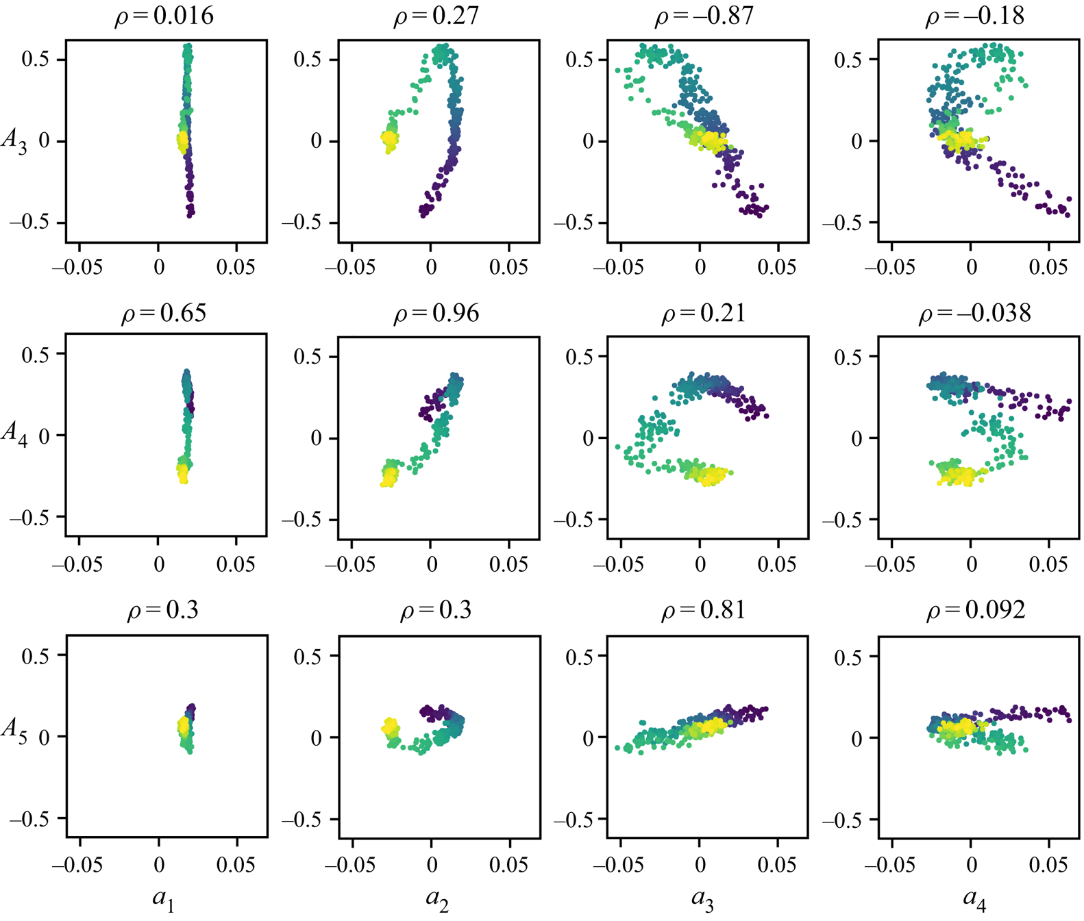
Figure 15. Correlation plots of the cosine coefficients  $A$ and the POD coefficients $a$ with the respective Pearson's correlation coefficients $\rho$ for case $\mathcal {S}$.
In summary, the POD provided coherent structures to generate a model concept for the reconfiguration events. It includes constant (mode 1) and reversing (mode 2) fractions of the flow structure. Modes 3 and 4 represent details of the two reversals processes of mode 2, which are dependent and independent from the reversal direction, respectively. In particular, the separation of the superimposed forced flow (mode 1) allowed us to consider these events as buoyancy-induced flow reversals with an accumulation and release process.
The correlation plots of the latter two modes showed that there is a correlation of these modes and the cosine fit amplitudes which describe the translation mechanism. Nevertheless, the causal connection cannot be deduced from the modes’ coherent structures in an obvious manner. Therefore both concepts, translation and switching, represent projections of a complex underlying flow process. Thus, their connection should be further investigated in the future.
4.3. Velocity fields of continuous reconfigurations
As discussed in § 4.1, the wavenumbers 7, 8 and 9 are dominant at certain times of a reconfiguration cycle for the smaller Richardson number  $Ri_{\mathcal {C}}=1.5$. In figure 16(a), we depict coefficient $A_8$, which showed the largest amplitudes, to emphasise how the acquired flow fields are associated with the cycle. The graph shows approximately six cycles of varying amplitudes of which just over four were covered by PIV. Six exemplary flow fields of that measurement are shown in figure 16(b) analogous to § 4.2.
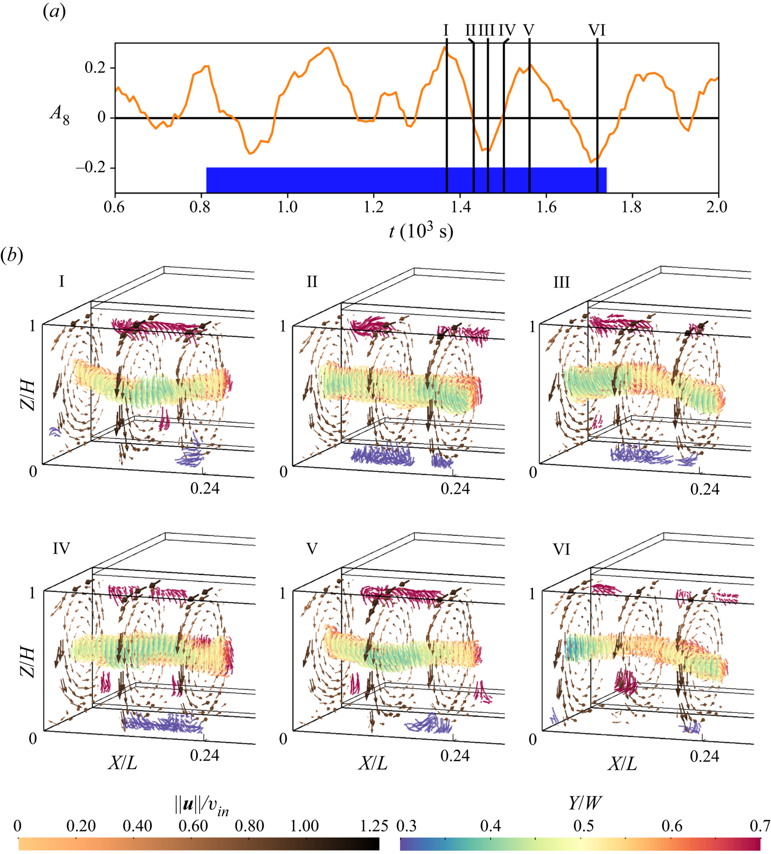
Figure 16. (a) Time series of the wavenumber amplitudes over the course of a reconfiguration event. The interval for which velocity fields were measured is marked by a blue bar. (b) Velocity fields for 6 points in times, which are indicated in the temperature series. The fields are represented by vectors in 3 cross-sections and streamlines in areas of  ${\|\boldsymbol {u}\|}/{v_{in}}<0.2$, which reflect the convection roll core. The displayed fields are short-time averaged over 25 frames. The complete time series can be seen in supplementary movie 5.
Snapshot I shows a convection roll which is straight in relation to the different alignments of case  $\mathcal {S}$. However, with regard to the color-coded $Y$-positions, it is possible to observe a displacement towards the rear at the sides of the measurement volume and towards the front at $X \approx L/8$. That equals a doubled number of distinct diagonal alignments in the PIV domain in comparison with case $\mathcal {S}$. It further matches the dominant wavenumber $w=8$ derived from the temperature data by the cosine fits. For snapshot II, there are no roll displacements from the centre. This coincides with a constant decline and zero crossing of $A_8$. The next snapshot (III) relates to a minimum of $A_8$ and shows the opposite displacements in the velocity field as compared to I. Snapshot IV completes the cycle since it again represents a zero crossing of $A_8$ with no roll displacement observable in the corresponding velocity field. To demonstrate the repeatability, the snapshots V and VI show similar roll core arrangements as I and III. Both pairs represent a maximum and a minimum of $A_8$, respectively.
Just as in case  $\mathcal {S}$, this case also shows a switching of the diagonal roll alignment, whereas the analysis of the temperature data indicates a translation. However, this case is characterised by different associations of the hot and cold regions at the rear wall with the main roll's $Y$-displacement: by comparing the implied temperature distribution of $A_8$ with the velocity fields, we found that warmer regions are associated with areas where the convection roll's core is displaced towards the rear. This is the opposite behaviour compared to the $\mathcal {S}$ case.
To better understand this observation, it is necessary to gain insight into the coherent structures of this flow by applying a POD to the velocity fields. Above all, these roll core displacements are superimposed by erratic fluctuations which have nearly the same amplitude as the displacement in the exemplary snapshots, as supplementary movie 5 associated with figure 16(b) shows. This emphasises the need for a filtering analysis of the flow structures also represented by the POD. Following the same approach as in § 4.2, the eigenvalue distribution as well as the normalised structure of the most prevalent modes is depicted in figure 17.
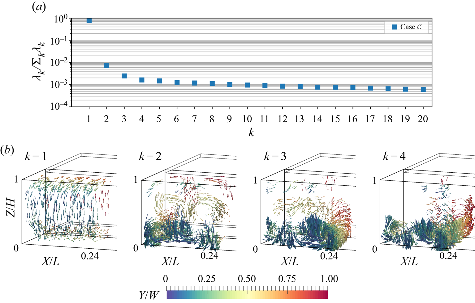
Figure 17. Eigenvalue distribution for the POD of case  $\mathcal {C}$ (a) and the four most prevalent modes normalised by the square root of the respective eigenvalue (b). Their structure is represented by the vectors of the highest magnitude. Supplementary movie 6 contains tracking shots of the displayed structures.
For this case, the first mode includes significantly more energy (79 %) than the first mode of case  $\mathcal {S}$ (60 %). Since a larger amount of energy is concentrated within this mode, less energy is allocated to the following modes compared to their equivalents of case $\mathcal {S}$. For instance, the contribution of the second mode is already smaller than 1 %. This corresponds to the smaller Richardson number of case $\mathcal {C}$, as it signals that the inertial forces, which support the structure of the first mode, are even more dominant for this case.
Similar to case  $\mathcal {S}$, the second mode incorporates coherent structures with rotation axes parallel to the $Y$-axis. In contrast to the single circulation which spreads across the whole domain for case $\mathcal {S}$, we observe six smaller circulations for the $\mathcal {C}$ case. Their arrangement, two rolls in the longitudinal direction and three of these pairs in the vertical direction of the domain, was similarly found by Westhoff (Reference Westhoff2012, pp. 57–59).
Modes 3 and 4 also display vortical structures, whose rotation axes are parallel to  $Y$. However, their strongest contribution is limited to one layer of vortices above the bottom plate. Together with mode 2 and with regard to Brunton & Kutz (Reference Brunton and Kutz2019, pp. 396–397), these structures represent the translation of vortices in this lower layer. This motion is not transferred to the centre of the sample, as contributions of modes 3 and 4 are weak in this region and a switching can be observed. Our analysis of these modes is limited to their structure, as the time development coefficients of modes with lower eigenvalues appear increasingly noisy.
Superimposing the first two modes yields, similar to case  $\mathcal {S}$, diagonally aligned convection roll segments in the centre $XY$-plane. Regarding mode 2, only the circulations at central $Z$-positions influence the alignment of the core of forced convection structure of mode 1, which is positioned at the same height. This explains the difference between both cases regarding the association of warm regions at the rear wall and the displacement of the convection roll core: while the centre pair of rotating coherent structures controls the roll displacement, the counter-rotating bottom structures affect the air reaching the temperature sensors.
In order to assess whether roll segments of this case perform a switching motion during reconfigurations, we consider the time development coefficients displayed in figure 18. Again, the first mode has a constant coefficient of just under  $0.02$, signalling a consistent contribution of the main forced convection roll structure to the flow. Whereas the second mode shows fluctuations around zero with varying amplitudes. The changes of sign of this mode's coefficients indicate that the direction of the coherent structures of mode 2 reverses for case $\mathcal {C}$, too. That means that the overall convection roll alignment switches as in case $\mathcal {S}$, but with the doubled spatial wavenumber.
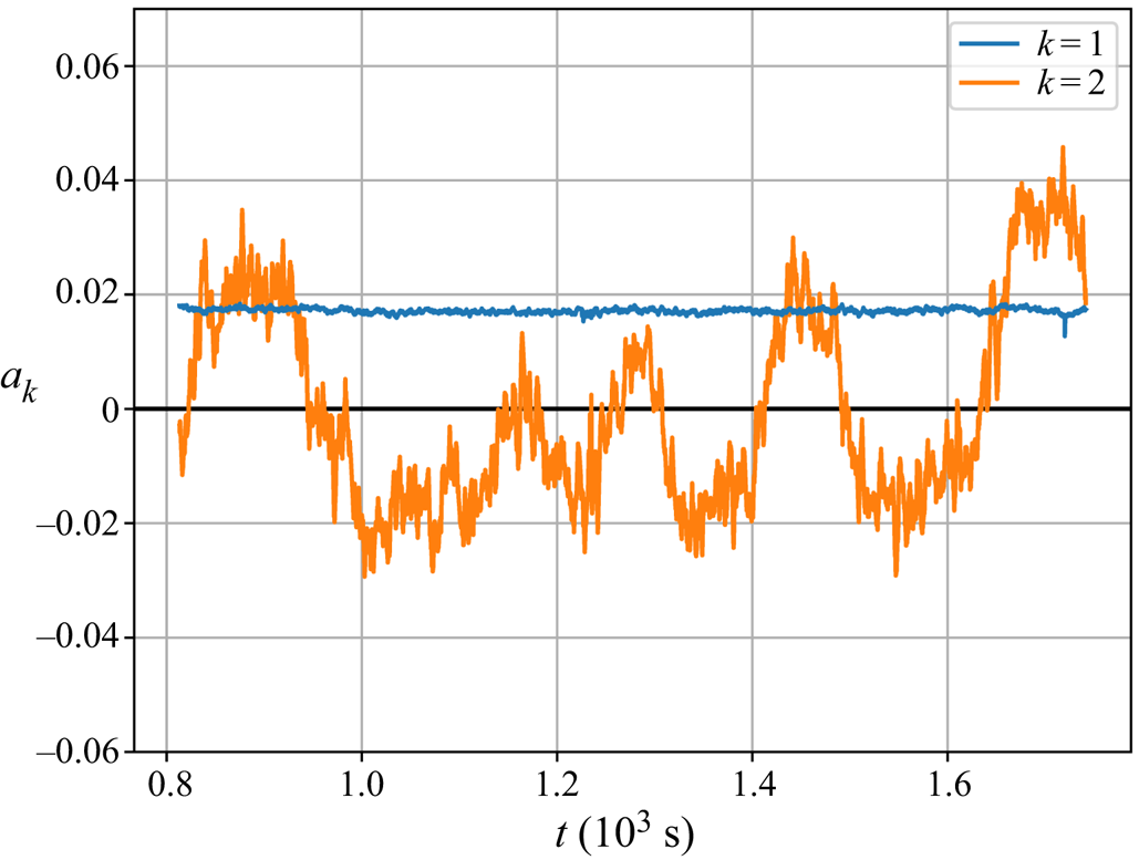
Figure 18. Time development coefficients for the first 2 POD modes also displayed in figure 17.
The relation between velocity and temperature fields is investigated by means of correlation plots presented in figure 19. The strongest correlation occurs with  $|\rho _{A_8a_2}|=0.83$ which confirms that the lower $Y$-parallel roll pair of mode 2 is responsible for the appearance of LSC-indicating hot spots at the rear wall.
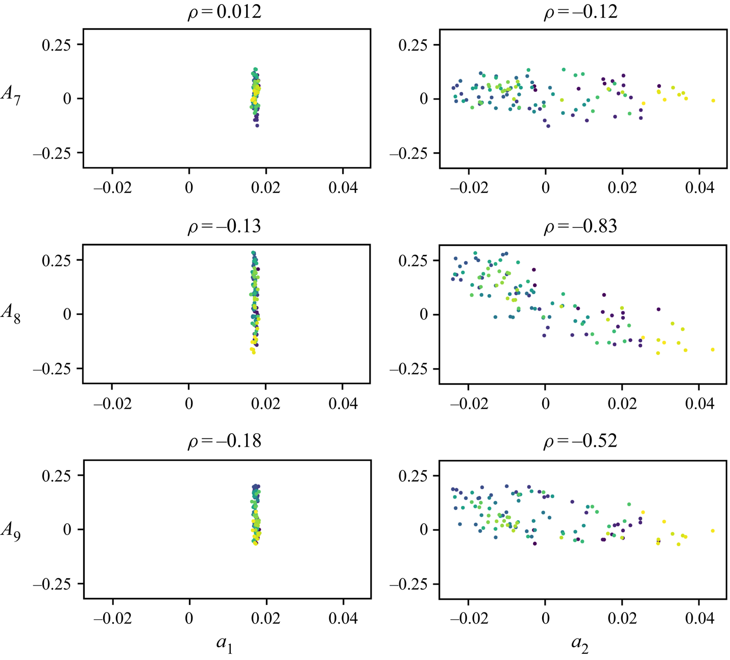
Figure 19. Correlation plots of the cosine coefficients  $A$ and the POD coefficients $a$ with the respective Pearson's correlation coefficients $\rho$ for case $\mathcal {C}$.
As stated in § 4.1, the characteristics of the temperature fit parameters indicated a mechanism driven by forced flow. The second mode in case  $\mathcal {C}$ confirms this concept: the strong bottom pair of coherent structures of this mode has a similar appearance as Taylor–Görtler-like vortices appearing in lid-driven or open cavity flows (Koseff & Street Reference Koseff and Street1984; Iwatsu et al. Reference Iwatsu, Ishii, Kawamura, Kuwahara and Hyun1989). Both studies show that these structures can occur with a size of $H/3$ for $Re$ numbers of the same magnitude as those of the present study.
These structures originate from a Görtler or Taylor instability as the down-welling flow follows concave streamlines bending towards the bottom plate near the front edge of the sample. Both instabilities are based on an unstable radial stratification of the flow's angular momentum (Strutt Reference Strutt1917; Taylor Reference Taylor1923; Görtler Reference Görtler1954). Yet, the Taylor and Görtler numbers are tailored to determine the onset of unstable behaviour for the respective flows and are thus unsuitable to explain the different behaviour of the two present cases. Therefore, we apply the Rayleigh criterion for stability ( $\varPhi >0$) presented by Chandrasekhar (Reference Chandrasekhar2013, pp. 273–275). In order to compare both cases, the stability discriminant $\varPhi = ({1}/{r^3})\nabla_{\boldsymbol {r}}(r\,\|\boldsymbol {u}\|)^2$ is calculated for the flow fields averaged over complete respective time series. These fields are similar to the first modes and thereby contain the longitudinal roll structure from which Taylor–Görtler-like vortices eventually arise. All details regarding the definition of $\varPhi$ can be found in appendix A.
Figure 20 shows the  ${\varPhi }$ fields in a representative cross-section at $X=L/8$. For both cases, regions of unstable angular momentum stratifications ( ${\varPhi }<0$) can be found next to the edge vortices in the top and bottom left corners of the cross-sections, where the vortex boundaries (see appendix A) are highlighted by green contour lines. The decisive difference between the cases is that the instability regions occurring for case $\mathcal {C}$ at the bottom edge vortex are stronger and larger. Integrating the regions of negative $\varPhi$ next of the bottom edge vortex yields $-0.018\ \mathrm {m}^2\,\textrm {s}^{-2}$ for case $\mathcal {S}$ and $-0.056\ \mathrm {m}^2\,\textrm {s}^{-2}$ for case $\mathcal {C}$. This proves that the centrifugal forces, which can induce Taylor–Görtler-like vortices, are significantly stronger for the low $Ri$.
$Ri$.
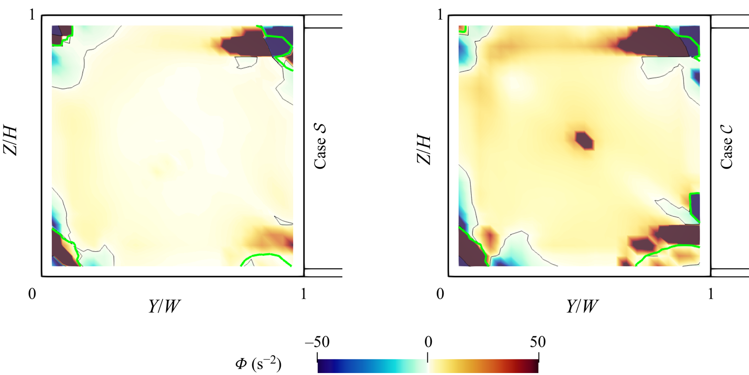
Figure 20. Value of  ${\varPhi }$ at $X=L/8$ of the average velocity field for both cases. The thin black contour line highlights the change of sign. The thicker green contour indicates the extent of the edge vortices, as it shows where the $X$-curvature equals zero.
To sum it up, the different behaviour of both cases can be attributed to the different manifestations of their longitudinal convection rolls. While they appear similar in figures 11 and 17, the different relation between thermal and forced convection causes the inlet jet to curve dissimilarly around the front edges of the sample and consequently to develop different angular momentum gradients.
Besides displaying similar vortex structures as case  $\mathcal {C}$, open cavity flow also holds analogies for the observed dynamic behaviour of these structures. Douay, Pastur & Lusseyran (Reference Douay, Pastur and Lusseyran2016) and Picella et al. (Reference Picella, Loiseau, Lusseyran, Robinet, Cherubini and Pastur2018) presented cases of these flows where sidewall effects lead to an instability of the arrangement of Taylor–Görtler-like vortices. Such effects lead to Bödewadt flow (Schlichting & Gersten Reference Schlichting and Gersten2016, pp. 329–330). However, this type of flow alone would induce a movement of the structures from the centre to the sidewalls of the sample. Hence, this mechanism can only function as an initial stimulus, while the switching process is then driven by an interaction of both buoyancy and inertial forces. Therefore, future research should focus on the proposed interaction, for example with parameter studies regarding the exact onset of this reconfiguration type.
5. Conclusion and outlook
Mixed convection flow in a cuboidal sample was investigated for two cases of different Richardson numbers,  $Ri_{\mathcal {S}}=3.7$ and $Ri_{\mathcal {C}}=1.5$, in order to determine to what extent concepts of RBC can be transferred to the occurring spontaneous or continuous flow reconfigurations. An initial rear-wall temperature analysis allowed us to allocate different prevalent numbers of LSCs, namely $w_{\mathcal {S}}=4$ and $w_{\mathcal {C}}=8$, to the cases. For both cases, the temperature measurements confirmed the translation of the structures observed by Schmeling et al. (Reference Schmeling, Bosbach and Wagner2013). We showed that this translation can be described by fitting a sum of cosine functions to the temperature distribution. The time evolution of the fit parameters implied – in accordance with earlier findings – that the apparent translation is accompanied by dissolving and emerging LSCs near the sidewalls. However, 3-D PIV measurements of the volume next to the left sidewall were analysed for both cases and showed that the translation mechanism cannot be transferred to the dynamics of the velocity structures. Instead, a switching of the observable diagonal section(s) over the course of a reconfiguration was identified.
In accordance with RBC in rectangular samples, a secondary circulation in shape of a convection roll branch was found for the case of spontaneous reconfigurations ( $\mathcal {S}$). However, it rather manifests a given LSC structure than it influences the reconfiguration process. The POD of the observed $\mathcal {S}$-type event extracted a set of influential modes. One mode represented a large fraction of the thermally forced flow as it resembles the flow structure of pure RBC. It allowed us to consider the switching of a diagonal LSC as superposition of constant forced flow combined with a reversal of the thermal flow components. Furthermore, the time evolution of the cosine and POD coefficients revealed that a process of accumulation and release is the underlying reconfiguration concept of this case. In particular, the events are associated with the release of multiple strong plumes from the front bottom edge vortex.
The POD results for the continuous reconfiguration case ( $\mathcal {C}$) showed that the second mode also supports the concept of switching diagonals, which was observed in the velocity fields of this case, too. The second mode's structure of vertically stacked coherent circulations further explained the opposite relation between convection roll displacement and hot spots in comparison with case $\mathcal {S}$. The stacked structures additionally indicated that this case including its reconfigurations is mainly driven by forced convection. We found that these structures form due to the predominant influence of the Taylor or Görtler instability. A consideration of similar structures in open cavity flow shows that secondary instabilities provided also explanations for the onset of reconfigurations of this structure.
Correlations between the different time coefficients obtained from the temperature and velocity fields showed that the respective second mode covers the formation of the prevalent temperature structure for both cases. However, many aspects of the relation between the different flow structure dynamics, translation of temperatures and switching of velocities, are still not understood. Future research should focus on the coupling of both mechanisms and on how the different states affect the heat transport in the sample.
Overall this study showed that certain concepts of RBC are transferable to mixed convection. As case  $\mathcal {S}$ showed, it is possible to approximate the reconfigurations as a reversal of the thermal fractions of the flow, while the forced fractions remain constant. However, this simplification is only valid for high enough $Ri$. This was shown by the investigation of the low- $Ri$ case $\mathcal {C}$, which had nearly the same $Ra$ as case $\mathcal {S}$ but showed completely different coherent structures.
This raises the question of a critical  $Ri$ for this distinction, as it may not necessarily be bound to the reconfiguration type and is therefore a topic for future research. Future investigations should also focus on confirming the implications for the complete sample which are so far only extrapolations, due to the technical limitations of 3-D PIV. The present study provides an important prerequisite, as the knowing the three-dimensional structure of a complete LSC provides the basis for interpretation of future two-dimensional measurements covering the complete sample.
Acknowledgements
The authors thank A. Köhne for her support provided by proofreading the manuscripts.
Declaration of interests
The authors report no conflict of interest.
Supplementary movies
Supplementary movies are available at https://doi.org/10.1017/jfm.2020.705.
Appendix A. Calculation of the Rayleigh criterion discriminant
In § 4.3, the reason for the existence of Taylor–Görtler-like vortices is explained by comparing the fields of the Rayleigh criterion discriminant  $\varPhi = (1/r^3)\nabla_{\boldsymbol{r}}(r\, \|\boldsymbol{u}\|)^2$. This definition is a modification of the definition in cylindrical coordinates by Chandrasekhar (Reference Chandrasekhar2013, pp. 273–275)
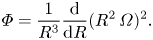 \begin{equation} \varPhi = \frac{1}{R^3} \frac{\textrm{d}}{\textrm{d}R} (R^2\, \varOmega)^2. \end{equation}
The origin of this cylindrical coordinate system with the radius coordinate  $R$ is assumed to be the centre of an analysed vortex. As the position of this centre is not per se known, we replaced $R$ by the local curvature radius $r$ and its associated unity vector $\boldsymbol {r}$. The latter is used for the directional derivative of the squared angular momentum term $(R^2\varOmega )^2$, where the azimuthal velocity $\varOmega = {\|\boldsymbol {u}\|}/{r}$ is replaced by the velocity magnitude $\|\boldsymbol {u}\|$, as each velocity vector is tangential to its local rotation.
In order to calculate the local curvature radii, we refer to Theisel (Reference Theisel1996, pp. 22–23). As a first step, the curvature vector  $\boldsymbol {\kappa }$ is calculated as follows:
 \begin{equation} \boldsymbol{\kappa} = \frac{\boldsymbol{u} \times \boldsymbol{\dot{u}}}{\|\boldsymbol{u}\|^3}. \end{equation}
 This introduces the time derivative  $\boldsymbol {\dot {u}}$ of the velocity vector. As we analyse single vector fields as steady states, it is reduced to the convection term
 \begin{equation} \boldsymbol{\dot{u}} = (\boldsymbol{u} \boldsymbol{\cdot} \boldsymbol{\nabla}) \boldsymbol{\cdot} \boldsymbol{u}. \end{equation}
 The local radius  $r$ and its unity vector $\boldsymbol {r}$ are then calculated as follows:
 \begin{gather} r = \frac{1}{\|\boldsymbol{\kappa}\|}, \end{gather}
 \begin{gather}\boldsymbol{r} = \frac{\boldsymbol{u} \times \boldsymbol{\kappa}}{\|\boldsymbol{u} \times \boldsymbol{\kappa}\|}. \end{gather}
For figure 20, these equations were applied in paraview, which calculates derivatives for the cells inscribed by the grid points of the vector field. These cell values were then interpolated to the original grid to complete the calculations. The curvature vector was further used to highlight the boundaries of the edge vortices, which we defined as  $\kappa _X=0$.


 Open access