


Introduction
Motion parameters of a micro-electro-mechanical system (MEMS), such as frequency and modal vectors, are crucial in optimizing process structures and enhancing the device performance. However, conventional detection methods are difficult to implement since MEMS devices are not only designed in millimeters or even smaller sizes, but also vibrate at a high frequency (kilohertz/megahertz) with a small amplitude (micron/nanoscale units) (Niu et al., Reference Niu, Li, Qi and Guo2019). So many optical techniques have been used and one of the most popular is the laser Doppler vibrometer (LDV) with nanometer precision. However, it is mainly used for out-of-plane motion detection and has limited application, as it can only detect one point at a time. High-speed cameras and holograms can capture the full field of view, but they are not cost-effective. Conversely, the stroboscopic micro-visual system captures the transient image sequences of the MEMS devices with periodic in-plane motion in a direct and practical way. After acquiring the image sequences, an appropriate demodulation algorithm is also essential to effectively extract the motion parameters of the device. Jin et al. (Reference Jin, Jin, Li and Wang2009) proposed an optical flow algorithm, but large errors would occur if the ambient luminance changed during the period of the device's motion. Xie et al. (Reference Xie, Bai, Shi and Liu2005) demonstrated a novel sub-pixel template-matching (TM) algorithm based on cubic spline interpolation, but it was too slow for real-time detection. To address the issues raised above, the authors have proposed a new feature point matching (FPM) algorithm based on Speeded-Up Robust Features (SURF) in this paper. It extracts motion parameters from image sequences by matching identical features. Experimental results show that the proposed algorithm improved the demodulation precision by two orders of magnitude in the same processing time compared with the other two popular algorithms.
Experimental Setup
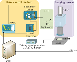
As shown in Figure 1a, the ultrafast stroboscopic micro-visual system mainly consisted of a light-emitting diode (LED) source, a drive control module, and an imaging system. In the microscope (DJY-880, manufactured by Dianying Optical Instruments Co. in Shanghai, China), a blue LED served as the ultrafast stroboscopic light source in place of the original halogen lamp. It was driven by a short pulse driver (LDV-V 03-100 V4.0 produced by PicoLAS) with a minimum pulse duration of 1 ns and a maximum repetition rate of 35 MHz. A field-programable gate array (FPGA) triggered the pulse driver through a level converter. The charge-coupled device (CCD) (E3IS PM produced by KUY NICE) captured the transient image sequences of the MEMS device in motion. The acquired images were saved on a computer via USB 3.0. The experimental setup in our laboratory is shown in Figure 1b.

Fig. 1. (a) Schematic of the ultrafast stroboscopic micro-visual system. (b) Experimental setup of the ultrafast stroboscopic micro-visual system.
The timing chart of the stroboscopic system is illustrated in Figure 2. The illumination time should be kept as short as possible to capture the transient image sequences of the periodically in-plane working MEMS devices. It was impossible for the CCD camera to obtain sufficient luminous flux for clear imaging in a single shot. Thus, the strobe signal was set to the same frequency as that of the MEMS device, measured by the LDV. This ensured that the same position could be exposed multiple times until the CCD acquired a clear image. The CCD was triggered to open prior to the output of the strobe pulse and close after acquiring a clear image at a point in the phase cycle. This feature eliminated the need for a high-frequency electronic shutter on the CCD, allowing for a more cost-effective field implementation of the micro-visual system. Then a phase delay of δ = 2π/n was added to the strobe pulse to acquire the image at the next position of the periodically moving MEMS device until n images of an entire period were acquired (Hart et al., Reference Hart, Conant, Lau and Muller2000; Pandey et al., Reference Pandey, Banerjee, Karkhanis and Mastrangelo2017). The dynamic periodic motion of a vibrating part could be observed and measured using this type of signal synchronization. The reason that the ultrafast stroboscopic system can acquire clear images of the MEMS devices vibrating at a high frequency is derived as follows.

Fig. 2. Timing chart of the stroboscopic system.
The displacement and velocity of the MEMS in-plane motion can be described by the following equation:
 $$\left\{\matrix{y = A\sin ( \omega t) \hfill \cr v = A\omega \cos ( \omega t) \hfill} , \right.$$
where A is the maximum amplitude of motion and ω is the angular frequency which can be calculated by the following equation:
 $$\omega = 2\pi f , $$
where f is the vibrating frequency of the MEMS device.
The maximum velocity of the motion is
 $$v_{\max } = A\omega , $$
and the displacement within the flash width of a single stroboscopic pulse is
 $$\Delta S = \int_{( -\Delta t/2) }^{\Delta t/2} {vdt = 2A\sin \displaystyle{\pi \over n}} = 2A\sin ( \pi f\Delta t) ,$$
where n is the number of image sequences captured during a MEMS device's motion cycle and Δt is the flash width of a single stroboscopic pulse calculated by the following equation:
 $$\Delta t = \displaystyle{1 \over {nf}} . $$
Supposed f = 500 kHz, n = 100, the calculated displacement ΔS was about 3.14 × 10⁻⁷ m, at least two orders of magnitude smaller than the resolution limit of human eyes (10−4 m), which satisfied the conditions for clear imaging.
So, the ultrafast stroboscopic photography utilizing 20 ns light pulses enabled the system to visualize the MEMS devices at a frequency of 500 kHz and acquired clear images of the in-plane motion well beyond the resolution limit of human eyes.
In-Plane Motion Demodulation Algorithm
The SURF-based FPM algorithm was developed to demodulate the motion parameters of the MEMS devices from the image sequences obtained above.
FPM Algorithm Based on SURF
Image matching, which matches the target regions of two or more images, has been widely used in many fields, such as target tracking (Zitová & Flusser, Reference Zitová and Flusser2003; Salvi et al., Reference Salvi, Matabosch, Fofi and Forset2006). And it also provides a possible way to demodulate the motion parameters of the MEMS devices. The image matching algorithms can be divided into two categories: the one based on grayscale and the one based on features. The grayscale-based one directly matches the original images with the image mask by comparing their similarities, which can be calculated by the grayscale information. It is shown to be quite compute-intensive, and many regions of the original image are calculated unnecessarily. The feature-based routine matches the feature points of the two images. It significantly reduces the computational cost as there are fewer feature points than pixels in an image. The three main steps of feature-based methods are feature point detection, feature point matching, matching information output.
As for feature point detection, the three most popular algorithms are scale-invariant feature transform (SIFT) (Lowe, Reference Lowe2004), SURF (Bay et al., Reference Bay, Tuytelaars and Gool2006), and oriented fast and rotated binary robust independent elementary features (BRIEF) with the whole routine abbreviated to ORB (Rublee et al., Reference Rublee, Rabaud, Konglige and Bradski2011). Compared with SURF, SIFT is more time-consuming and less stable, and ORB is insensitive to micro displacements (Banerjee et al., Reference Banerjee, Chaturvedi and Tiwari2019; Bansal et al., Reference Bansal, Kumar and Kumar2021). So, SURF was selected to detect the feature points in our proposed algorithm. Then the feature points of two images were matched according to the matching degrees calculated by Euclidean distance. The random sample consensus (RANSAC) model (Brown & Lowe, Reference Brown and Lowe2002; Zhao & Du, Reference Zhao and Du2004) was applied to eliminate the existing mismatched point pairs, and the motion parameters could finally be calculated.
SURF Feature Point Detection
The main flows of SURF feature point detection are shown in Figure 3.

Fig. 3. The flow chart of SURF feature point detection.
The core of SURF involves constructing a Hessian Matrix for each pixel of the image. In order to retain the scale invariance property of feature points, a Gaussian filter is applied to each image by convolving them with a Gaussian kernel, which can be described as follows (Li et al., Reference Li, Jiang, Ma, Guo, Yuan and Dai2019):
 $$L_{xx}( x, \;y, \;\sigma ) = G( x, \;y, \;\sigma ) \otimes I( x, \;y) , $$
 $$G( x, \;y, \;\sigma ) = \displaystyle{{\partial ^2} \over {\partial x^2}}\displaystyle{1 \over {2\pi \sigma ^2}}e^{( {-}x^2 + y^2/2a^2) }, $$
where I(x, y) is the pixel value of point (x, y) in the image, and G(x, y, σ) is the Gaussian kernel on the σ scale.
Then the Hessian matrix, which can be written as follows, is constructed to detect edges of the integral images:
 $$H( x, \;y, \;\sigma ) = \left[{\matrix{ {L_{xx}( x, \;y, \;\sigma ) } & {L_{xy}( x, \;y, \;\sigma ) } \cr {L_{xy}( x, \;y, \;\sigma ) } & {L_{yy}( x, \;y, \;\sigma ) } \cr } } \right] , $$
where L xx, L yy, and L xy are elements of matrix calculated by formula (6). The discriminant of the Hessian matrix is calculated to get the feature points at extreme values:
 $${\rm Det}( H) = \sigma ^4( L_{xx}( x, \;y, \;\sigma ) L_{yy}( x, \;y, \;\sigma ) -L_{xy}^2 ( x, \;y, \;\sigma ) ) .$$
It took a good deal of CPU time to compute the Gaussian function as it was required to be discrete and cropped in practical use. To reduce the processing time, box filters (Bay et al., Reference Bay, Tuytelaars and Gool2006) were employed in place of the Gaussian kernel, and the integral images were used in place of the original ones. Then formula (9) can be approximately written as follows:
 $${\rm Det}( H_{{\rm approx}}) = D_{xx}D_{yy}-( \omega D_{xy}) ^2 , $$
in which ω, usually set as 0.9, is the compensation coefficient of the box filter for the Gaussian kernel. The box functions D xx, D yy, and D xy correspond to the Gaussian kernel functions L xx, L yy, and L xy, respectively.
Different sizes of the box filters are applied to the images, and multi-scale image pyramids are built (Bay et al., Reference Bay, Tuytelaars and Gool2006). In order to localize feature points in the image and over scales, a non-maximum suppression is applied in a 3 × 3 × 3 neighborhood. If the Hessian matrix discriminant of a pixel, calculated by formula (10), is the maximum or minimum value compared to its neighbors, we save it as a feature point candidate. Interpolation in scale and image space is then applied to precisely obtain the position and scale value of feature points.
In order to be invariant to rotation, Haar wavelet responses are calculated, and SURF descriptors are built (Xie et al., Reference Xie, Li and Zhao2020).
Feature Point Matching
In feature point matching, the Euclidean distance between two sets of feature points, for which a smaller value means higher match quality, can be calculated as follows:
 $$D = \sqrt {\sum\nolimits_{i = 1}^n {{( x_{i1}-x_{i2}) }^2} } , $$
where x i1 is the ist coordinate of the first point and x i2 is the ist coordinate of the second point. The feature point pairs would be reserved if their Euclidean distance was below the setting threshold (Idris et al., Reference Idris, Warif, Arof, Noor, Wahab and Razak2019).
The flow chart of the FPM algorithm based on SURF is shown in Figure 4.

Fig. 4. The flow chart of FPM algorithm based on SURF.
After feature point detection and matching, there still existed some mismatched point pairs, and the RANSAC model was applied to eliminate them. The displacement between adjacent frames was then calculated by taking a weighted average of all the displacements calculated by each point pairs.
Experimental Results and Discussions
The images of the tested MEMS gyroscope, whose designed resonant frequency was 8.189 kHz, are shown in Figure 5. However, the maximum amplitude was an unknown parameter that must be characterized as the manufactured devices were not always consistent with the design criteria. Figure 5a was captured by the CCD camera under the halogen lamp as a light source, while Figure 5b under the ultrafast stroboscopic system. It is evident that the image of the vibrational region highlighted in the red box in Figure 5b is more distinguishable compared with the one in Figure 5a.

Fig. 5. Local images of the MEMS vibratory gyroscope. (a) Image captured by the CCD camera illuminated by the halogen lamp. (b) Image acquired by the ultrafast stroboscopic system.
The image sequences of the periodically in-plane working MEMS devices we captured included 190 frames. The FPM algorithm based on SURF was applied to acquire the velocities and displacements of the device. The demodulation area was limited to the region highlighted with the red box in Figure 5b since the entire area vibrated at the same speed. But for the part outside of the red box, only middle tooth structures in combs were vibrating, while others were static. It could introduce distortion to the demodulation calculation, which was not favorable. The processing time of all 190 frames was 100.85 ms. Therefore, the processing rate was 1884 fps, which could realize real-time detection. Experiments of the demodulation algorithms were conducted on a computer equipped with a Windows 10 operating system and an Intel i7-9700 F CPU. The required software environments were visual studio 2015 and its OpenCV 2.4.9 libraries. The curves of the displacements and velocities were constructed, which are shown in Figure 6.

Fig. 6. Motion parameters demodulated by FPM based on SURF. (a) The velocity curve of the MEMS gyroscope. The inset is an enlarged part to show the error bar area. The reduced χ 2 of sine fit is 0.00625; R 2 is 0.99596; and Adj. R 2 is 0.99589. (b) The displacement curve of the MEMS gyroscope. The reduced χ 2 of sine fit is 0.28380; R 2 is 0.99922; and Adj. R 2 is 0.99921.
The dominant noise in Figure 6a was caused by environmental vibration, which was depicted as the difference between the sine-fitting velocity curve and the measured one. Due to the random nature of environmental vibration, the displacements calculated by integrating the velocities averaged out the random noise as shown in Figure 6b. It had a minor difference between the fitted and measured data. According to the displacement curve of the MEMS gyroscope under test, the amplitude was 26.61 pixels, corresponding to 4.59 μm. This result matched well with the design parameter.
Other two commonly used gray-based motion demodulation algorithms, TM (Lai et al., Reference Lai, Lei, Deng, Yan, Ruan and Zhou2020; Wang et al., Reference Wang, Liu, Li, Li, Zha, He, Ma and Duan2020) and frame-differences (FD) (Li et al., Reference Li, Qiu, Lin and Zeng2006), were also developed to make a comparison with the FPM algorithm based on SURF. TM calculated the displacements by translating the template pixel by pixel from the top left to the bottom right of the image to find the best-matched position. The FD method also obtained the displacements by translating the adjacent frames pixel by pixel. Six of all 190 recorded frames were selected as a sample to be demodulated by the three different algorithms to compare the sub-pixel precision. The results are summarized in Table 1. With the same processing time, the precision achieved by the FPM algorithm based on SURF was 10−5 pixels, while that of the TM and the FD were 10−2 and 10−1, respectively. The precision of TM and FD algorithms could be further improved with interpolation algorithms, but would undoubtedly result in longer processing time.
Table 1. Vibrating Velocities Calculated by Different Demodulation Algorithms.

The vibrating velocity shown in Table 1 was defined as the relative displacement of the current frame to the previous one with a fixed sampling time. Since six frames were under the demodulation process, five relative displacements were calculated. The images of the MEMS devices were magnified by 20 times with an objective, and the pixel size of the Point Gray industrial CCD was 3.45 μm, from which we could calculate the actual image size of the pixel as follows:
 $$1\,{\rm pixel} = \displaystyle{{3.45\,\mu {\rm m}} \over {20}} = 172.5\,{\rm nm}. $$
Finally, the velocity curves demodulated by the three algorithms of all 190 frames are shown in Figure 7.

Fig. 7. Comparison of velocities calculated by the TM, FD, and FPM algorithms based on SURF.
As shown in Figure 7, all three algorithms could roughly demodulate the velocity curves. But at the extreme points, compared with the FPM based on SURF, the TM algorithm displayed more substantial fluctuation, and the demodulation of FD was distorted to some extent. Thus, the FPM method based on SURF achieved higher accuracy while demodulating the image sequences. Additionally, this was also shown from the quantitative R 2 results given in Table 2. The closer the R 2-value was to 1, the more consistent the fitting curve was with the data.
Table 2. R 2 of Different Demodulation Algorithms.

Conclusions
An ultrafast stroboscopic method using a 20 ns flash pulse was developed and implemented to obtain clear “frozen” images of the MEMS devices with in-plane vibration at kHz repetition rates, which overcame the limitation of the slow electronic shutter rate of the CCD. By utilizing the FPM method based on SURF, a precision of 10−5 pixels of the image was achieved, which was 2-magnitude higher than that of the TM and FD algorithms within the same processing time. The velocity and displacement curves of a MEMS vibratory gyroscope, which vibrated at a frequency of 8.189 kHz, were demodulated from the recorded images.
Funding
National Key Research and Development Program of China (2018YFF01013203).


