


INTRODUCTION
Meteorological factors have been recognized as risk factors associated with hand, foot, and mouth disease (HFMD) epidemics [Reference Song1–Reference Hii, Rocklöv and Ng3]. We previously demonstrated that in Wuhan, China, HFMD cases are frequently reported with temperatures of 10–25 °C and reports decrease at temperatures below 10 °C or above 25 °C [Reference Chen4]. This inverse V-shaped relationship between the reported number of HFMD cases and temperature has also been observed during HFMD epidemics in Taiwan and mainland China [Reference Chang5, Reference Liao6]. Our previous results suggest that bimodal seasonal peaks in HFMD epidemics are attributable to enterovirus A71 (EV-A71) epidemics. Current hypotheses explaining the seasonal pattern of EV-A71 infection include host immune competence fluctuations mediated by seasonal factors, such as melatonin or vitamin D levels [Reference Dowell7] as well as seasonal behavioural factors unrelated to weather, such as school attendance and indoor crowding [Reference Chang8]. However, human behavioural factors alone do not appear to account for the seasonal pattern observed in certain cases of EV-A71 infection, including those that occur among school-aged children or in association with household crowding [Reference Chang9].
It has been reported that viruses are devoid of thermostatic mechanisms and that their reproduction and survival rates are strongly affected by fluctuations in temperature, as are those of parasites and bacteria [Reference Meeburg and Kijllstra10, Reference Patz11]. Thus, investigation of the effect of meteorological factors on the epidemiology of infectious diseases, including HFMD, is necessary for practitioners and public health policy makers to control disease and for planning public health media events to promote preventive activities. Based on our previous study in Wuhan, China [Reference Chen4], controlling the spread of viral infections at temperatures ranging from 10 to 25 °C should be considered, to help prevent HFMD infections. In Japan, no concrete temperature range has been associated with HFMD epidemics. Many people believe that HFMD is an infection that occurs in the summer season, but the timing of such infections is too ambiguous to prevent and predict HFMD incidence. Further investigation is required to clarify the association between HFMD and meteorological conditions in Japan.
The purpose of this study was to further clarify the association between HFMD epidemics and meteorological conditions. For this, we used HFMD surveillance data of all 47 prefectures in Japan, collected by Japan's National Epidemiological Surveillance of Infectious Diseases (NESID) [Reference Harigane12]. Japan extends from latitude 45°N to 20°N; therefore, meteorological conditions vary widely. We considered that a subset of the HFMD surveillance data might be useful to clarify the association between HFMD epidemics and meteorological conditions.
Our study used HFMD surveillance data and meteorological data of all prefectures in Japan, based on a study conducted in Japan's southern prefectures reporting that ambient temperature and relative humidity were associated with increased occurrence of HFMD [Reference Onozuka and Hashizume13]. To precisely estimate the relationship between HFMD data throughout Japan and meteorological data, we proposed a method with a clear criterion of adequate estimation. The analyses included spectral analysis using the maximum entropy method (MEM) and least squares method (LSM) [Reference Ohtomo14, Reference Sumi15]. The obtained results might assist in the prediction of epidemics and preparation for the effects of climatic changes on infectious disease epidemiology.
DATA
HFMD data
The time series data analysed in this study represent the weekly reported HFMD incidence data for all 47 prefectures of Japan. These data were obtained from the Infectious Diseases Weekly Report Japan [16]. The incidence data for each prefecture indicates the number of HFMD cases reported weekly per paediatric sentinel clinic in the prefecture. There are approximately 3000 paediatric sentinel clinics nationwide. The number of sentinel clinics (3000) has been set to a standard error rate of annual number of HFMD patients in all of Japan of <5% [Reference Nagai17]. Sentinel HFMD cases were defined by clinical presentation, that is, papular or vesicular rash on the hands, feet, mouth, or buttocks, with or without fever [16]. The data for each prefecture were gathered over 835 weeks (835 data points) from January 2000 to December 2015. Portions of the 2011 data for Miyagi Prefecture (week 10) and Fukushima Prefecture (weeks 10, 11, 13, and 14) were unavailable because of the Great East Japan Earthquake. These missing data were replaced with the mean values, which were calculated using the data immediately before and after the missing observations. The 47 prefectures of Japan are shown in Figure 1.
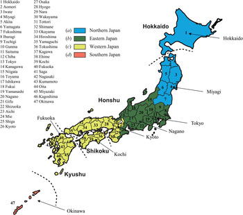
Fig. 1. Distribution of the 47 prefectures of Japan. Dashed lines indicate boundaries of the four main islands constituting Japan: Hokkaido, Hoshu, Shikoku, and Kyushu. The eight prefectures are used as representative sites: (a) Hokkaido and Miyagi Prefectures in northern Japan (blue); (b) Tokyo and Nagano in eastern Japan (green); (c) Kyoto, Kochi, and Fukuoka in western Japan (yellow); and (d) Okinawa in southern Japan (orange).
Meteorological data
The Automated Meteorological Data Acquisition System (AMeDAS) developed by the Japan Meteorological Agency (JMA) is a high-resolution surface observation network. The AMeDAS comprises 1300 stations throughout Japan, of which 840 stations cover temperature, relative humidity, precipitation, and so on; the average distance between stations is 21 km [18]. In the present study, we used daily data collected at the AMeDAS stations in the 47 prefectural capitals. These data were obtained from the JMA website [19] and included average temperature, maximum temperature, minimum temperature, relative humidity, and precipitation. Daily data were obtained for a total of 5845 days from 2000 to 2015 (5845 data points).
Descriptive statistics for the weekly meteorological data are shown in Table 1. Notably, the mean values of average temperature rise with lower latitudes: 9·3 °C in Hokkaido (latitude 43°N), 12·8 °C in Miyagi (38°N), 16·7 °C in Tokyo (35°N), 12·3 °C in Nagano (36°N), 16·2 °C in Kyoto (35°N), 17·4 °C in Kochi (33°N), 17·4 °C in Fukuoka (33°N), and 23·3 °C in Okinawa (26°N).
Table 1. Summary statistics for weekly meteorological conditions of eight prefectures in Japan used as representative site

METHODS
Selection method of eight prefectures as representative sites
Based on geographical division by the JMA [19], we selected eight from among the 47 prefectures in Japan as representative sites. For providing weather information, the JMA divides the entire country into the following four areas: northern, eastern, western, and southern Japan. In this study, we selected one, two, or three prefectures from each area as illustrative examples (Fig. 1), as follows: (a) Hokkaido and Miyagi from northern Japan; (b) Tokyo and Nagano from eastern Japan; (c) Kyoto, Kochi, and Fukuoka from western Japan; and (d) Okinawa from southern Japan; this gave a total of eight prefectures. Among them, Hokkaido has a subpolar climate and Okinawa has a subtropical climate. The other six prefectures (Miyagi, Tokyo, Nagano Kyoto, Kochi, and Fukuoka) have a temperate climate [Reference Donald Ahrens20].
Figure 1 shows the results for eight of the representative sites. In Table 1, the eight prefectures are arranged from northern to southern Japan by latitude and longitude.
Data analysis
Setting up the time series data for analysis
The sampling interval differed for the HFMD data (weekly) and meteorological data (daily). To analyse these two datasets together, it was necessary to choose equal sampling intervals. Therefore, we calculated weekly data for the meteorological variables (835 data points) from the original daily data (5845), to conform to the weekly HFMD data. All meteorological parameters studied and values used for testing the associations are summarized as supplementary information (see online Supplementary Table S1). For example, the weekly average maximum temperature was calculated by averaging the daily maximum temperature for 1 week. The weekly meteorological variables are as follows: T{A}, average temperature (°C); T{M}, maximum temperature (°C); T{m}, minimum temperature (°C); RH, relative humidity (%); RF, total rainfall (mm).
To explain the present method, we used weekly HFMD data of Fukuoka Prefecture (Fig. 2a ), which is located in western Japan (Fig. 1).

Fig. 2. Procedures of the present analysis method, where incidence data of Fukuoka Prefecture are used an example. (a) Weekly incidence of HFMD per sentinel clinic from 2000 to 2015. (b) Average occurrence of HFMD infections against average temperature (T{A}), N T{A} in equation (1). (c) Power spectral densities of N T{A}. (d) Comparison of the least squares fitting curve X T{A}(Temp) in equation (4) (solid line) with the original data N T{A} in equation (1) (dashed line).
Correlation between HFMD data and meteorological data
The average occurrence of HFMD in the different domains of average temperature (T{A}), T to T + ΔT, was calculated using the following formula [Reference Chan21]:
 $$N_{T\left\{ {\rm A} \right\}} = \displaystyle{{\sum\nolimits_i^n {C_if(t_i)}} \over {\sum\nolimits_i^n {\,f(t_i)}}}, $$
where i is the sequence from 0 to n (=834, corresponding to the data point [835] minus one), t i is T{A} for the ith week period, C i is the total number of disease cases per sentinel clinic in the ith week, and f(t i ) is a function with the following values:
 $$f\,(t_i)\left\{ \matrix{ = 1,\,{\rm when}\,T \le t_i \lt T + \Delta T \hfill \cr = 0,\,{\rm otherwise} \hfill} \right.$$
The numerator on the right side of equation (1) represents the sum of all C i comprising the 1-week average temperature (t i ) within the temperature domain of T to T + ΔT during the data period. The denominator is the total number of occasions in which T < t i < T + ΔT is satisfied during the same data period.
Similarly, average occurrences of HFMD infections in the different variable domains for maximum temperature (N T{M}), minimum temperature (N T{m}), RH (N RH), and RF (N RF) were determined. The variables t i , T, and ΔT for T{A} in equations (1) and (2) were replaced with tM i , TM, and ΔTM, respectively, for T{M}; with tm i , Tm, and ΔTm, respectively, for T{m}; with h i , H, and ΔH, respectively, for RH; and with r i , R, and ΔR, respectively, for RF. Values for ΔT, ΔTM, ΔTm, ΔH, and ΔR were determined using semi-empirical procedures, as previously described [Reference Chen4]; these were 1, 1, 1 °C, 5%, and 30 mm, respectively. As a result, we obtained temperature-dependent incidence data (N T{A}, N T{M}, and N T{m}), RH-dependent incidence data (N RH), and RF-dependent incidence data (N RF).
In Figure 2b , we show the temperature-dependent incidence data, that is, the value of N T{A} against Temp [temperature (°C)] for Fukuoka Prefecture.
Spectral analysis and LSM
(i) Theoretical background. We assumed that temperature-dependent incidence data, N T{A} against Temp (Fig. 2b ), was composed of systematic and fluctuating parts [Reference Armitage, Berry and Matthews22]:
 $$N_{T\left\{ {\rm A} \right\}} = {\rm systematic}\,{\rm part} + {\rm fluctuating}\,{\rm part}$$
The systematic part in equation (3) is regarded as the underlying variation in the original data; the fluctuating part, including undeterministic components such as noise, was obtained as the residual data when the underlying part was subtracted from the original data. Estimation of the underlying variation is a key point.
The underlying variation in the original data N T{A} against Temp (Fig. 2b ) is assumed to be described by the function X T{A}(Temp), as follows:
 $$\eqalign{X_{T{\rm \{ A\}}} (Temp) & = A_0 \cr & \quad + \sum\limits_{i = 1}^N {A_i\cos \{ 2\pi f_i(Temp + \theta _i)\}},}$$
which is calculated using the LSM for N T{A} with unknown parameters f i , A 0, and A i (i = 1, 2, 3, …, N), where f i (=1/T i ; T i is the period) is the frequency of the ith component, A 0 is a constant that indicates the average value of N T{A}, A i and θ i are the amplitude and phase of the ith component, respectively, and N is the total number of components. The values of N were determined using a semi-empirical procedure, as previously described [Reference Chen4]. In the same manner, the formulations of the least squares fitting (LSF) curve to N RH and N RF are described by the function h [RH (%)] and by the function r [RF (mm)], respectively, as follows:
 $$X_{{\rm RH}}(h) = A_0 + \sum\limits_{i = 1}^N {A_i\cos \{ 2\pi f_i(h + \theta _i)\}}, $$
 $$X_{{\rm RF}}(r) = A_0 + \sum\limits_{i = 1}^N {A_i\cos \{ 2\pi f_i(r + \theta _i)\}.} $$
The LSM using equations (4)–(6) must be non-linear. Linearization of this non-linearity is required to obtain unique optimum values of these parameters. In the present study, linearization of equations (4)–(6) is achieved using the MEM-estimated frequency f i .
(ii) Determination of f i (spectral analysis). To estimate f i in equation (4), spectral analysis based on MEM was conducted for N T{A} against Temp (Fig. 2b ). Spectral analysis has been applied to spatial series data [Reference Mattfeldt23, Reference Mise24] and time series data [Reference Sumi25, Reference Sumi26]. MEM spectral analysis has a high degree of resolution and is useful for clarifying periodicities within short data series, such as the data examined in this study [Reference Sumi25, Reference Sumi26]. Formulation of the MEM power spectral density (PSD) is described in the Appendix.
The value of f i in equation (4) is determined by the position of the spectral peak in the PSD, shown in Figure 2c . In the figure, prominent spectral lines were observed at f = 0·022 and f = 0·057, which corresponded to 45·5 and 17·5 temperature periodic modes, respectively, owing to a large difference between the beginning and end parts of the data and asymmetrical pattern of the data N T{A} against Temp (Fig. 2b ).
(iii) Determination of A 0, A i and θi, and N (least squares analysis). Using two frequency modes (N = 2), f = 0·022 and f = 0·057 observed in Figure 2c with X T{A}(Temp) in equation (4), the optimum values for parameters A 0, A i , and θ i (i = 1, 2) in equation (4) are determined exactly from the optimum LSF curve calculation. In Figure 2d , the LSF curve X T{A}(Temp) thus calculated is shown with the original data N T{A}.
The reproducibility level of N T{A}, N T{M}, and N T{m} by equation (4), N RH by equation (5), and N RF by equation (6) were evaluated by Pearson's correlation (ρ) using IBM SPSS Statistics for Windows, Version 22·0 (IBM Corp., Armonk, New York, USA). A two-tailed analysis was used for all statistical tests and a P value of ⩽0·05 was considered statistically significant.
RESULTS
Case description
From January 2000 to December 2015, a total 2 521 199 cases of HFMD were reported in Japan. Children under 5 years of age accounted for over 80·4% of the reported cases from 2000 to 2014 [16].
Temporal variations in HFMD data
The eight weekly incidence datasets gathered from January 2000 to December 2015 are shown in Figure 3. All weekly incidence data showed an annual cycle. For Okinawa (Fig. 3h ), bimodal cycles of epidemics were clearly observed in 2002 and 2011.

Fig. 3. Weekly incidence of HFMD per sentinel clinic from 2000 to 2015, in eight prefectures of Japan: (a) Hokkaido, (b) Miyagi, (c) Tokyo, (d) Nagano, (e) Kyoto, (f) Kochi, (g) Fukuoka, and (h) Okinawa.
Correlations between HFMD cases and T{A}, T{M}, and T{m}
Using HFMD data (Fig. 3) and data for T{A}, T{M}, and T{m}, we obtained N T{A}, N T{M}, and N T{m} [equation (1)], respectively. The results of N T{A} are shown in Figure 4, and those of N T{M} and N T{m} are listed in the Supplementary Material (see online Supplementary Figs S1 and S2, respectively).

Fig. 4. Average occurrence of HFMD infection against average temperature (T{A}), N T{A} in equation (1), and its least squares fitting curve, X T{A}(Temp) in equation (4). X T{A}(Temp), solid line; N T{A}, dashed line. (a) Hokkaido, (b) Miyagi, (c) Tokyo, (d) Nagano, (e) Kyoto, (f) Kochi, (g) Fukuoka, and (h) Okinawa.
We conducted MEM spectral analyses for N T{A} for the eight prefectures; MEM-PSDs are shown in Figure 5. In each PSD, two prominent spectral lines were observed. By using the two periodic modes for each prefecture observed in Figure 5, the optimum LSF curve, X T{A}(Temp) [equation (3)], to N T{A} data (Fig. 4) was calculated; the X T{A}(Temp) thus obtained is shown in Figure 4. Therein, X T{A}(Temp) for each prefecture reproduces the underlying variation of N T{A} data. The optimum LSF curves for N T{A}, N T{M}, and N T{m} [X T{A} (Temp), X T{M}(Temp), and X T{m}(Temp), respectively] were similarly calculated using two dominant periodic modes in the PSDs, which are listed in the Supplementary Material (see online Supplementary Table S2). The good fit of the LSF curves to the data of N T{A}, N T{M}, and N T{m} was supported by the result that the values of ρ covered the upper level: ρ = 0·83–0·97 for N T{A}, ρ = 0·87–0·96 for N T{M}, and ρ = 0·83–0·99 for N T{m}.

Fig. 5. Power spectral densities of N T{A}. (a) Hokkaido, (b) Miyagi, (c) Tokyo, (d) Nagano, (e) Kyoto, (f) Kochi, (g) Fukuoka, and (h) Okinawa.
In the LSF curves for N T{A}, that is, X T{A}(Temp), of the eight prefectures (Fig. 4), the patterns showed positive slopes against Temp. Notably, in Fukuoka Prefecture (Fig. 4g ), for example, X T{A}(Temp) indicated a maximum value at Temp = 28 °C and decreased at 28 °C < Temp. This inverse V-shaped relationship between X T{A}(Temp) against Temp was observed in 21 of the 47 prefectures (45%). For cases that exhibited inverse V-shaped slopes, we estimated maximum values of X T{A}(Temp) and inflection points or minimum values just before the maximum values of X T{A}(Temp). Maximum values of X T{A}(Temp) ranged from 24 to 30 °C (Fig. 6a ), and inflection points or minimum values of X T{A}(Temp) ranged from 12 to 18 °C (Fig. 6b ). Each set of the values shown in Figure 6a , b for X T{A}(Temp) indicated no significant correlations with latitude of the prefectures.

Fig. 6. Number of prefectures against temperature for X T{A}(Temp), X T{M}(Temp), and X T{m}(Temp). (a) Number of prefectures against temperature for maximum value of X T{A}(Temp), (a′) number of prefectures against temperature for maximum value of X T{M}(Temp), (b) number of prefectures against temperature for inflection point or minimum value of X T{A}(Temp), and (b′) number of prefectures against temperature for inflection point or minimum value of X T{m}(Temp).
In the LSF curves for N T{M}, that is, X T{M}(Temp) (online Supplementary Fig. S1), an inverse V-shaped relationship between X T{M}(Temp) against Temp was observed for 26 of the 47 prefectures (55%). Maximum values of X T{M}(Temp) are shown in Figure 6a′. It is worth noting that the maximum values ranged from 28 to 35 °C, a higher temperature range compared with the case of X T{A}(Temp) (24–30 °C) (Fig. 6a ).
In the LSF curves for N T{m}, that is, X T{m}(Temp) (online Supplementary Fig. S2), an inverse V-shaped relationship between X T{m}(Temp) against Temp was observed for 15 of the 47 prefectures (32%). Inflection points or minimum values of X T{m}(Temp) are shown in Figure 6b′. Interestingly, inflection points or minimum values ranged from 6 to 17 °C, a lower temperature range compared with the case of X T{A}(Temp) (12–18 °C) (Fig. 6b ). Among all 47 prefectures, there were 12 in which both X T{m}(Temp) and X T{M}(Temp) were assigned, as listed in Table 2. Both X T{m}(Temp) and X T{M}(Temp) listed in Table 2 showed no significant correlations with latitude of the prefectures.
Table 2. Prefectures where both XT{M}(Temp) and XT{m}(Temp) were assigned, and the values of each prefecture's XT{M}(Temp) and XT{m}(Temp)

Correlations between HFMD cases and RH
Using the HFMD data (Fig. 3) and RH data, we obtained N RH [equation (1)]; the results of N RH are shown in Figure 7. We investigated the LSF curves of N RH, that is, X RH(h) [equation (5)], using the same procedure as with the cases of N T{A}, N T{M}, and N T{m} (Fig. 4); the results of X RH (h) for the eight prefectures are shown in Figure 7. For all cases, the value of N RH gradually increased with increasing RH > 60%. In Miyagi (Fig. 7b ), for example, the value of X RH (h) peaked at h = 80% and decreased at 80% < h. This inverse V-shaped relationship between X RH (h) against h was observed for eight of 47 prefectures (17%). Maximum values of X RH (h) ranged from 70% to 85% (Fig. 8a ), and inflection points or minimum values ranged from 45% to 70% (Fig. 8b ). Each set of the values shown in Figure 7a , b for X RH (h) indicated no significant correlations with latitude of the prefectures.


Fig. 8. Number of prefectures against relative humidity (RH) for X RH(h). (a) Number of prefectures against relative humidity for maximum value of X RH(h), and (b) number of prefectures against temperature for inflection point or minimum value of X RH(h).
Correlations between HFMD cases and RF
Using data of HFMD (Fig. 3) and RF, we determined N RF [equation (1)]; the results are displayed in Figure 9. We calculated the LSF curves of N RF, that is, X RF (r) [equation (6)], by following the same procedure as that for N T{A}, N T{M}, and N T{m} (Fig. 4); results of X RF (r) for the eight prefectures are shown in Figure 9. For Miyagi, Tokyo, and Kyoto (Fig. 9b, c and e , respectively), the values of X RF (r) increased with increasing r < 300 mm. For Kochi, Fukuoka, and Okinawa (Fig. 9f–h , respectively), the values of X RF (r) still increased at 300 mm ⩽ r: 270 mm ⩽ r < 360 mm for Kochi (Fig. 9f ), 270 mm ⩽ r < 420 mm for Fukuoka (Fig. 9g ), and 360 mm ⩽ r < 480 mm for Okinawa (Fig. 9h). With respect to Hokkaido and Nagano (Fig. 9a , d, respectively), it was difficult to find a relationship between X RF (r) and r because of a relatively small amount of rainfall.

DISCUSSION
The present results for T{A} demonstrated a lower threshold at 12 °C (Fig. 6b ) and a higher threshold at 30 °C (Fig. 6a ). This supports our previous result that the risk of HFMD infection is high at 10 °C ⩽ Temp < 25 °C in Wuhan, China [Reference Chen4]. However, the results for T{M} and T{m} indicated a lower threshold at 6 °C (Fig. 6b′) and a higher threshold at 35 °C (Fig. 6a′). These findings can help with control of HFMD at temperatures 6 °C ⩽ Temp ⩽ 35 °C, which is a wider temperature range than 12 °C ⩽ Temp ⩽ 30 °C for T{A} (Fig. 6a, b ). Based on this result, we recommend the use of maximum and minimum temperatures rather than the average temperature, to estimate the temperature threshold of HFMD infections.
Many studies have found threshold effects between meteorological factors and HFMD epidemics [Reference Song1–Reference Liao6]. Our findings showed that for 26 and 15 of the 47 prefectures, the risk function of T{M} and T{m}, respectively, approximated an inverse V-shaped curve with HFMD incidence, and the threshold of temperature ranged from 6 to 35 °C (Fig. 6a′, b′ ). This association may be partially explained by the fact that temperatures ranging from 2 to 27 °C provide a more favourable environment for enterovirus epidemics [Reference Salo and Cliver27], making it easier for people to be infected. However, extreme temperatures may make it difficult for people to take part in public activities, which makes them less likely to be infected [Reference Liao6].
For RH, there was a lower threshold at 45% and a higher threshold at 85% (Fig. 8a, b ). This result supports that of Zhang et al. [Reference Zhang28], who found a threshold of RH ranging from 45% to 85% in Shenzhen, China. Within a certain range of RH, higher humidity could facilitate viral attachment to the surface of objects, including toys [Reference Wong29], which is also supported by experimental studies wherein viruses exhibit a rapid rate of decline during the dry season [Reference Abad, Pinto and Bosch30].
For rainfall (Fig. 9), our findings of a positive correlation between reported cases of HFMD and rainfall in all cases, except for Hokkaido and Nagano (Fig. 9a, d , respectively), are supported by our previous study. In that study, we demonstrated that Wuhan, China, which is in an area with a subtropical wet monsoonal climate, experiences more outbreaks of HFMD during the rainy season [Reference Chen4]. The large values of X RF (r) at 300 mm ⩽ r for Kochi and Fukuoka in western Japan (Fig. 9f, g , respectively) and Okinawa in southern Japan (Fig. 9h ) might result from typhoons, which often land and develop in these areas during July–November, as well as the East Asian rainy seasons during June–July in early summer and during November–December in early winter.
Until recently, EV-A71 and coxsackievirus A16 (CA16) have been considered the main causes of HFMD in Japan. However, in 2009, coxsackievirus A6 (CA6) began to emerge as a cause of HFMD. Large HFMD outbreaks in the country were caused by CA6 in 2011, 2013, and 2015. Among the prefectures investigated in this study, bimodal seasonality of HFMD was observed in Okinawa Prefecture in southern Japan (Fig. 1). The causative agent of HFMD in Okinawa is not known because only 26 strains of enterovirus have been reported in Okinawa between 1986 and 2016. As a result, the bimodal seasonality of HFMD in Okinawa in 2002 and 2011 is yet to be explained. Because the average value of T{m} in Okinawa (21·1 °C in Table 1) is above 6 °C, Okinawa is the only prefecture that belongs to the subtropical zone in Japan. It is possible that the bimodal HFMD epidemics in Okinawa can be explained by multiple epidemics of CA16, EV-A71, and CA6 within 1 year. One good example of unique enterovirus circulation in Okinawa is a local outbreak of haemorrhagic conjunctivitis that was caused by coxsackievirus A24 (CA24) [Reference Harada31]. No outbreaks of CA24 were observed in Japan, except for in Okinawa, during the period of this study.
Using HFMD surveillance data collected in all 47 prefectures by Japan's nationwide surveillance system for infectious diseases, we confirmed that there is no latitude dependence of maximum values, and inflection point or minimum value of X T{A}(Temp), X T{M}(Temp), X T{m}(Temp) (Fig. 6), and X RH (h) (Fig. 8). The country is divided into prefectures, each of which is further subdivided into cities with respective wards and blocks. In the present study, we used prefecture data of HFMD because prefecture measures are the minimum unit of measurement released by the NESID in Japan. To investigate spatial characteristics of HFMD incidence in Japan in more detail, such as the spatial heterogeneity [Reference Liao32, Reference Liu33], further studies using data from cities, wards, and/or blocks should be conducted.
Causative pathogens of HFMD, such as EV-A71, CA16, and CA6, may affect the disease duration or epidemic peaks [Reference Lum34, Reference Tnag35]; however, in the present study, there was no information available on these pathogens. Under this condition, the use of equations (1) and (2) in this study enabled us to efficiently examine whether HFMD transmission in the 47 prefectures was related to meteorological factors. Information on the causative agents of HFMD for each Japanese prefecture can assist in future investigation of those meteorological factors related to HFMD transmission in the country, using more sophisticated methods such as generalized additive models [Reference Huang36] and non-linear regression models [Reference Takahashi37].
A limitation of the present study is that we used weekly data of HFMD, whereas we used daily data for meteorological factors, because weekly measures are the minimum unit of measurement released by the NESID. We investigated monthly HFMD and meteorological data for Fukuoka Prefecture to compare the results shown in Figure 2d . We confirmed that, with monthly data, we did not obtain the inverse V-shaped curves obtained for weekly data (see online Supplementary Fig. S3). Furthermore, we confirmed that, for the eight prefectures (Fig. 3), the variance of yearly temperature was relatively small compared with the variance of yearly incidence rate of HFMD (see online Supplementary Table S3). Thus, we consider that the monthly and yearly data are too rough to extract a correlation between HFMD data and meteorological data. Further studies using daily data of HFMD should be conducted.
In conclusion, we demonstrated that the ambient temperature and relative humidity thresholds can be extracted from NESID data of the 47 prefectures in Japan by constructing a systematic procedure with a clear criterion of adequate estimation. We recommend the use of maximum and minimum temperatures to estimate the temperature threshold of HFMD epidemics. The obtained results might aid in the prediction of HFMD epidemics and preparation for the effect of climatic changes on HFMD epidemiology.
SUPPLEMENTARY MATERIAL
The supplementary material for this article can be found at https://doi.org/10.1017/S0950268817001820.
APPENDIX
MEM spectral analysis
MEM-PSD P(f) (where f represents frequency) for the time series with equal sampling interval ∆t, can be expressed by
 $$P(\,f) = \displaystyle{{P_m\Delta t} \over {{\left \vert {1 + \sum\nolimits_{k = - m}^m {\gamma _{m.k}\exp \left[ { - i2\pi fk\Delta t} \right]}} \right \vert} ^2}},$$
where the value of P m is the output power of a prediction-error filter of order m and γ m, k is the corresponding filter order. The value of the MEM-estimated period of the nth peak component T n (=1/f n ; where f n is the frequency of the nth peak component) can be determined by the positions of the peaks in the MEM-PSD.
ACKNOWLEDGEMENTS
The authors thank Analisa Avila, ELS, from Edanz Group (www.edanzediting.com/ac) for editing a draft of this manuscript. This study was supported by JSPS KAKENHI, Grant Numbers JP16K09061, JP25460769, JP25305022.
ETHICAL STANDARDS
This study was approved by the Ethical Committee of the National Institute of Infectious Diseases on 8 January 2015.


