


Introduction
Microwave filters are key components of current and future communication systems. The steadily increasing data rates of such systems lead to two effects, which affect the filter design process. On the one hand, the center frequency (especially in e.g. satellite communications) tend to increase which require smaller components and hence higher efforts in the manufacturing. On the other hand, the crowded electro-magnetic spectrum leads to stringent filter requirements in terms of near and far out-of-band rejection.
Transmission zeros (TZs) allow to fulfill at least the out-of-band rejection specifications as well as group delay restrictions in quasi-elliptical filter responses [Reference Cameron1]. Several techniques are known for their realization: frequency-dependent (dispersive) coupling apertures can be a meaningful approach, especially if “negative” cross-couplings should be avoided [Reference Szydlowski, Leszczynska, Lamecki and Mrozowski2, Reference Szydlowski, Lamecki and Mrozowski3]. In this context, a negative cross-coupling is a coupling aperture which realizes a different sign as the main-line couplings of the filter. A commonly used structure for waveguide filters is a partial height post [Reference Szydlowski, Lamecki and Mrozowski3, Reference Politi and Fossati4] or coupling apertures which are able to couple electric and magnetic fields simultaneously [Reference Rosenberg, Amari and Seyfert5]. However, for an application in the W-band or at higher frequencies these apertures are very small and therefore are not always suitable for manufacturing. Another alternative is the use of extracted pole filters. The TZ-generating cavity is designed as a hanging (extracted pole) resonator which usually couples to the main path of the filter by a non-resonating node [Reference Cameron, Kudsia and Mansour6–Reference Amari and Macchiarella8]. Disadvantageously, the position of the TZ determines the required coupling factor between the non-resonating node and the extracted pole cavity. If the TZ is placed far away from the passband, the coupling factor often tends to unrealistically large values. The realization of extracted pole filters is therefore mostly accomplished in a H-plane design and limited to TZs near to the passband [Reference Leal-Sevillano, Montejo-Garai, Ke, Lancaster, Ruiz-Cruz and Rebollar9, Reference Xiao, Li and Sun10].
Filters based on bypass couplings (e.g. the singlet or doublet approach) for the realization of TZs in the near passband vicinity are a meaningful alternative [Reference Amari, Rosenberg and Bornemann11, Reference Ding, Shi, Zhou, Zhao, Liu and Wu12]. However, in the high-frequency range the design possibilities are severely limited. For example, the number of individual components should be as low as possible in order to avoid alignment problems and additional loss generated by contact resistances. The approach proposed in [Reference Bastioli, Tomassoni and Sorrentino13] is therefore not optimal for W-band applications.
In this paper, three fourth-order filters are proposed, which reveal up to seven real frequency axis TZs. These TZs are realized by combining several TZ-generating effects:
• A cross-coupling of non-adjacent cavities is used to realize a symmetric pair of real frequency axis TZs close to the passband.
• Due to the chosen filter structure bypass couplings arise, which accomplish a further TZ in the vicinity of the passband.
• The source to load (SL) cross-coupling is able to realize TZs by classical destructive interference as well as dispersive TZs, which arise due to the distance of the aperture from the source/load port. The frequency of the TZs can be varied with dependence on the position of the SL coupling aperture [Reference Miek, Reinhardt, Daschner and Höft14, Reference Miek, Morán-López, Ruiz-Cruz and Höft15].
The combination of these effects in the proposed filters allows the utilization of up to seven TZs, partially spread over the whole W-band. Especially, TZs far away from the passband might be useful to suppress narrow-band signals which may arise as an intermodulation product from an amplifier. Design charts for proper positioning of the TZs are given within this paper. The use of SL couplings reveals several advantages, especially at high-frequency ranges, where the required manufacturing tolerances are often stringent. As will be shown, up to four TZs can be added to the filter response by manufacturing a coupling aperture with proper dimensions in order to connect the source/load port. The manufacturing of this coupling is comparably easy and the desired rejection specifications might be fulfilled without using additional resonators or diagonal cross-couplings. Furthermore, adding an SL coupling has only small influence on the return loss level of the filter. The first design can therefore be accomplished conventional without this coupling and the de-tuning effect can be compensated by a final optimization. As will be shown in this paper, the rejection properties of a filter can be varied heavily especially by using asymmetric TZs.
The orientation of the manufacturing cut additionally influences the arrangement of the cavities and, therefore, the performance of the filters in terms of number of TZs, quality factor, spurious mode performance, and manufacturing accuracy. All these topics are addressed within this paper and examined on three similar fourth-order W-band filters.
This paper is organized as follows: in Section “Filter set-ups,” the filter specifications are defined and the basic set-ups (without SL coupling) are discussed. The coupling matrices of all filters are presented and manufacturing issues are addressed. Section “Improved filter responses by using source–load couplings” investigates the effect of adding a direct SL cross-coupling to the filter set-ups. Design charts for the positioning of the cross-coupling aperture are given in this section. The measurement results are compared to the simulation in Section “Measurement results and comparison,” and Section “Spurious mode performance” analyzes the spurious mode performance of the different filters with and without an SL coupling. A tolerance analysis of all proposed set-ups is accomplished in Section “Tolerance analysis” and finally Section “Conclusion” summarizes and concludes this paper.
Filter set-ups
Three filters are designed with similar specifications to ease the comparison. All of them are fourth-order filters with a return loss of at least RL = 20 dB in the passband. The center frequency is f 0 = 87.7 GHz and the bandwidth is B ≈ 1 GHz. Two symmetrically placed TZs are foreseen in the initial designs. One possible filter set-up to meet the TZ specification is shown in Fig. 1(a). The filter consists of four cavities, where the first and third cavities are designed to resonate at the TE 102 mode while cavities two and four are realized as standard TE 101 mode cavities. This filter set-up was already proposed in [Reference Miek, Morán-López, Ruiz-Cruz and Höft15, Reference Miek, Boe, Kamrath and Höft16] for Ku-band applications. The design is straightforward and is based on coupling matrix extraction and tuning techniques [Reference Cameron, Kudsia and Mansour6, Reference Hong and Lancaster17].

Fig. 1. Overview of the similar filter set-ups with different cutting planes: (a) filter 1 with H-plane cut in the x–z plane, (b) filter 2 with cut in the y–z plane (the coupling apertures between cavity 1/4 and 2/3 are realized by holes in a metal foil of thickness t = 0.1 mm) and (c) filter 3 with cut in the x–z plane (the cavities are stacked above each other and are separated by a thin metal foil as well). The effect of adding the SL cross-coupling is investigated in Section “Improved filter responses by using source–load couplings.”
The magnetic fields of the first set-up are shown in Fig. 2. Note that the fields along the main path of the filter are oppositely oriented to each other. This orientation eases the evaluation of the sign of the coupling factor, which is proportional to

where i, j indexes two neighboring cavities. In accordance with this definition and the fields in Fig. 2, the couplings along the main path are counted positive while destructive interference of the magnetic fields between cavities one and four arises. This leads to a negative cross-coupling and realizes the desired symmetrical pair of real frequency axis TZs. The basic idea of using oversized cavities for a sign change was first proposed in [Reference Rosenberg18]. In the case presented here, cavity three rotates the direction of the magnetic field and therefore enables a negative coupling between cavities one and four. Resonator one is therefore not required to be an oversized cavity. However, to improve the mechanical stability and increase the Q-factor, this cavity resonates with the TE 102 mode as well. As will be discussed in Section “Measurement results and comparison,” each filter is realized with and without a direct SL cross-coupling. For the sake of completeness, this SL cross-coupling aperture is already depicted in the drawings of Fig. 1.

Fig. 2. Magnetic fields in the filter set-up from Fig. 1(a) in accordance with [Reference Miek, Boe, Kamrath and Höft16].
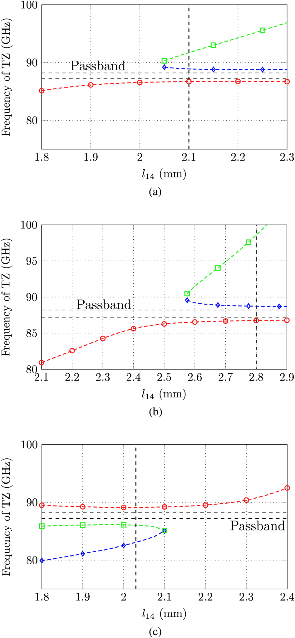
Additionally, bypass couplings propagate over the TE 101 modes in the oversized cavities one and three and finally realize the topology in Fig. 3. The bypass couplings lead to an additional TZ in the vicinity of the symmetric TZ pair. The frequency of this TZ can be varied by e.g. adapting the width (d 14) or position (l 14) of the cross-coupling aperture (compare Fig. 1). This will, however, also influence the position of the TZs generated by the quadruplet. A parameter study regarding the positioning of the third TZ is shown in Fig. 4(a). As can be seen, large values of the parameter l 14 realize three TZs. By increasing the distance l 14, it is possible to shift the TZ which is created by the bypass couplings further away from the passband of the filter. Small values of l 14 realize a complex pair of TZs due to constructive interference of cavities one and four. The filter which was manufactured here as a prototype has a value of l 14 ≈ 2.1 mm (marked in Fig. 4(a)) and d 14 = 0.95 mm.

Fig. 3. Coupling topology of the filters in Fig. 1.
The set-up in Fig. 1(a) is realized as an H-plane filter (termed as “filter 1”). The complete filter structure can be realized in one component while only an additional flat cover-plate is required. The cutting plane is therefore along the x–z axis. Advantageously, a potential misalignment between both components should not affect the filter performance. Otherwise, the ridge separating cavity one/two from cavity three/four is relatively small and may lead to manufacturing inaccuracies. The simulation results of this filter are shown in Fig. 5(a) in comparison with the S-parameters generated by the coupling matrix of Table 1. This coupling matrix was obtained by optimization using the topology in Fig. 3 [Reference Amari, Rosenberg and Bornemann19]. It is worth mentioning that the position of the third TZ was chosen arbitrarily due to mechanical aspects of the filter design process, for example, large values of l 14 might lead to mechanical instability of the center structure which separates all of the cavities if d 14 is kept constant.

Fig. 5. Simulated S-parameters in comparison with the S-parameters generated by the coupling matrices in Tables 1–3. (a) Filter 1 from Fig. 1(a), the inset shows a photograph of the filter (housing and flat cover). (b) Filter 2 from Fig. 1(b), the inset shows a photograph of the two filter halves and the metallic foil in between. (c) Filter 3 from Fig. 1(c), the inset shows a photograph of the two filter halves and the metallic foil in between.
Table 1. Coupling matrix of filter 1 without SL cross-coupling

Other cutting planes for the realization of the similar topology are possible. Filter 2 in Fig. 1(b) is manufactured in three parts, where cavities one and two are separated from cavities three and four by using a thin metallic foil. The cutting plane coincides therefore with the y–z axis. The foil has a thickness of t = 0.1 mm, in which all required coupling apertures can be drilled. With this strategy the “ridge” from the first filter is conveniently avoided as the coupling takes place by holes in the metal foil. Otherwise, the aspect ratio of the structures to be milled is very high as now a channel of depth a = 2b but only a width b must be milled. In the case of filter 1 (H-plane cut) the depth is only b. Additionally, for this design it is critical that the three parts are properly aligned to each other. The simulation results in comparison with the S-parameters generated by the coupling matrix are shown in Fig. 5(b). Figure 4(b) reveals that the third TZ above the passband can be varied by the distance l 14 as well. Obviously, the slope is larger, allowing a higher flexibility in the positioning of this TZ. In the case of filter 2, the position was chosen as l 14 = 2.8 mm and the coupling iris has a diameter of d 14 = 0.8 mm. A potential coupling matrix of the proposed configuration is given in Table 2.
Table 2. Coupling matrix of filter 2 without SL cross-coupling

Finally, Fig. 1(c) shows the third filter which is based on a stacked cavity approach. The cutting plane is set along the x–z plane, identical as in the case of filter 1. However, now the cavities are stacked above each other and are coupled by a metallic foil similar to the second set-up. Again, cavities one and two are placed in the lower part while cavities three and four are positioned in the upper part. Contrary to filters 1 and 2, the coupling of the cavities takes place through the bottom/cover instead of the sidewall. This filter combines some advantages of both former filters: the aspect ratio is similar to the case of the first filter while otherwise no difficult structures like the “ridge” in the center of the four cavities as in filter 1 must be realized. Otherwise, the filter is again segmented into three parts and the correct alignment is critical. The simulated S-parameters are shown in Fig. 5(c) in comparison with the S-parameters generated by the coupling matrix in Table 3. The TZ realized by the bypass couplings is now below the passband at 82.5 GHz and might be moved by varying the distance l 14. For this prototype l 14 = 2.03 mm and d 14 = 0.55 mm was chosen (compare Fig. 5). The position of the TZ below passband must be attributed to a sign change of the bypass couplings due to the electrical cross-coupling between cavities one and four. Note that this coupling aperture is centered in cavity four and allows a primary electric coupling rather than a magnetic coupling as in the case of filters 1 and 2. A further TZ at 106 GHz arises, which cannot be explained by the topology from Fig. 3 and must be assigned to higher order mode resonances.
Table 3. Coupling matrix of filter 3 without SL cross-coupling

All filters are manufactured by using computer numerical control (CNC) milling techniques. Brass is used for the fabrication due to the good machining properties. The metal foil of the second and third filters is realized in brass as well. The insets in Figs 5(a)–5(c) show photographs of the manufactured filters.
Improved filter responses by using source–load couplings
A direct SL cross-coupling aperture can be added to all three filter set-ups as already suggested in Fig. 1. The minimum path rule gives a theoretical upper bound for the maximal available number of TZs n fz, which is limited by the filter order n and hence defines the bound n fz,max = n [Reference Cameron, Kudsia and Mansour6]. In waveguide technology, the maximal number of TZs might be further increased by adding an SL cross-coupling with some distance to the filters input/output coupling. This effect was e.g. described in [Reference Mokhtaari, Bornemann, Rambabu and Amari20] for dual- and triple-band filters and utilized in [Reference Miek, Reinhardt, Daschner and Höft14] for a stacked W-band filter.
The distance l 0 of the SL cross-coupling aperture from the source or load port therefore has a large influence on the wide-band S-parameter response and the rejection properties. A comprehensive parameter study regarding the number and position of TZs in dependency of the distance l 0 is shown in Fig. 6 (compare Fig. 1). As can be seen, a periodic pattern of the TZ positions can be identified.

Fig. 6. Study of the position of all TZs in dependency of the shift l 0 from the input coupling of the source port: (a) filter 1 in Fig. 1(a) with d SL = 0.56, (b) filter 2 in Fig. 1(b) with d SL = 0.5, and (c) filter 3 in Fig. 1(c) with d SL = 0.5. The dashed lines indicate the position l 0 at which an SL coupling was introduced in the filters which are realized as a proof of concept.
Considering first Fig. 6(a), where the position of all TZs of the first filter from Fig. 1(a) is investigated in dependency of the parameter l 0. As can be seen, this structure can simultaneously generate up to six TZs in a frequency range between 75 and ~96 GHz. The red and blue lines mark the frequency of the TZs, which are generated by the cross-coupling of cavities one and four. These TZs are less affected by a variation of l 0, even if a small oscillation of the upper (blue) TZ curve can be observed in dependency of the distance of the nearest TZ above the passband. Moreover, it seems that periodically two TZs combine above the passband. If the distance l 0 is further increased, the TZs separate again below the passband. In order to achieve an improved rejection performance of the filter, a value of l 0 should be chosen which provides the maximal number of TZs while having the smallest distance from the source port. In the considered case, l 0 was chosen to 3.05 mm, which is also marked in Fig. 6(a).
A similar TZ pattern is generated by the second filter set-up of Fig. 1(b), which is shown in Fig. 6(b). Again, a combination of two individual TZs in the vicinity of the passband can be observed, which are separated again below the passband. However, due to the improved behavior below the passband, in total up to seven TZs can be utilized in a frequency range between 75 and 104 GHz. As will be discussed later, one filter set-up with l 0 = 2.9 mm was realized as a proof of concept.
Finally, Fig. 6(c) shows the TZ pattern of the third filter set-up from Fig. 1(c). This TZ pattern is clearly different from those in Figs 6(a) and 6(b). In this case, TZs arise over the entire W-band frequency region. This property might be useful, if narrow-band signals far away from the passband should be suppressed. Furthermore, only one TZ above the passband is more or less fixed. The TZ below the passband, which is generated by the quadruplet, can also be moved toward lower frequencies. In order to realize a high number of TZs, a filter set-up with l 0 = 5.575 mm was realized as a proof of concept.
Figure 7 compares the wide-band S-parameter responses of the filter set-ups from Fig. 1 with and without an SL cross-coupling.

Fig. 7. Rejection comparison of the different filters: (a)+(b) from filter 1, (c)+(d) from filter 2, and (e)+(f) from filter 3.
In Fig. 7(a) the transmission coefficient of the first filter (Fig. 1(a)) with SL coupling (red curve) is compared to that without SL coupling (blue curve). With the selected parameter combination (l 0, d SL) an improved rejection behavior in a wide area around the passband can be observed. Two TZs below and four TZs above the passband are achieved. Especially, above the passband a high rejection can be realized by the three consecutive TZs. Figure 7(b) shows the rejection improvement (RI) of the proposed configurations, which is defined as

An improvement compared to the set-up without SL coupling is achieved, if the curve is above 0 dB.
Obviously, the best improvement in terms of rejection can be achieved with filter 2 from Fig. 1(b), as can be seen in Figs 7(c) and 7(d). In total three TZs below and four TZs above the passband can be realized, which allow a rejection improvement over nearly the entire W-band frequency region.
Figures 7(e) and 7(f) finally compare the S-parameter responses of the stacked filter set-up from Fig. 1(c) with and without SL coupling. Even if in total six TZs might be realized by the set-up with SL coupling, there is no overall rejection improvement compared to the filter without SL coupling.
Measurement results and comparison
The filter set-ups from Fig. 1 are manufactured with the CNC milling technique as a proof of concept and for comparison purposes. The measurement results in comparison with the simulation are shown in Fig. 8. In total a set of six measurements are presented. Each filter set-up from Fig. 1 was realized once with and once without an SL cross-coupling. Note that only the H-plane filter from Fig. 1(a) must be manufactured two times as it requires milling of the SL-coupling in the cavity body. In case of the filters from Figs 1(b) and 1(c) an exchange of the centered metal foil is sufficient while the resonator housing can be reused.

Fig. 8. Measurement results in comparison with simulation. (a) and (b) show the results of the set-up in Fig. 1(a) without and with SL coupling, respectively. (c) and (d) show the results of the set-up in Fig. 1(b) without and with SL coupling, respectively. (e) and (f) show the results of the set-up in Fig. 1(c) without and with SL coupling, respectively.
Figure 8(a) shows the simulation results in comparison with the measurement for filter 1. In total three TZs can be observed. The TZs close to the passband are realized by the cross-coupling of cavities one and four while the third one arises due to bypass couplings in the oversized cavities one and three. The passband is visibly shifted toward lower frequencies. The reason for the center frequency shift is highly probable an outward spin of the cutter in the manufacturing process, which mainly increases the width of the cavities. This shift might be compensated without much effort in few iterations by reducing the width of all cavities. The return loss is decreased to ~7 dB due to further manufacturing tolerances, most probable due to the small ridge which separates the cavities. The H-plane filter with SL coupling (Fig. 8(b)) shows a similar behavior within the passband. A systematic manufacturing error is assumed to be the reason, as both filters have a similar filter structure but are manufactured independently from each other. However, it is possible to realize four consecutive TZs above the passband as predicted by the simulation (compare also Fig. 7(a)).
In Fig. 8(c) the measurement results for filter 2 (Fig. 1(b)) are shown. As an interesting result, no significant frequency shift is noticeable. The outward-drill, which probably enlarges the cavities of the first filter, may also arise by the manufacturing of this filter. However, the deviations arise in the y-direction, which does not influence the center frequency of the TE 101 or TE 102 mode due to the height independence. The measurement results of the set-up with SL coupling (Fig. 8(d)) show a behavior similar to the simulation. Three TZs below and four TZs above the passband can be noticed.
Finally, the measurement results of filter 3 (Fig. 1(c)) are shown in Figs 8(e) and 8(f). A smaller frequency shift compared to filter 1 arises due to the same reason as in the case of filter 1, but this might be compensated in few iterations if the filter is constructed with smaller cavities widths. The rejection behavior of both filter set-ups is close to the simulated ones.
Table 4 summarizes and compares important filter parameters. The unloaded Q-factor was estimated by using an adapted Cauchy extraction method as e.g. described in [Reference Macchiarella21]. Filter 1 shows a slightly higher Q-factor compared to filters 2 and 3, probably due to the filter structure which consists of only two components.
Table 4. Comparison of the results of the filter set-ups

The estimated unloaded Q-factor is given for the filter set-ups without an SL coupling. For the estimation the design center frequency and bandwidth is used.
Spurious mode performance
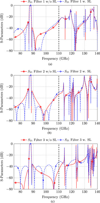
The spurious mode performance might be a major design criterion in specialized applications. Several techniques exist in order to shift the spurious modes as far away from the passband as possible, e.g. [Reference Wu, Zhu, Yang and Shi22, Reference Valencia, Boria, Guglielmi and Cogollos23]. The filters proposed here are not designed to fulfill certain rejection requirements above the W-band frequency range. However, it is worth to investigate if adding an SL coupling has a significant influence on the spurious mode performance of a filter. A comparison of the simulation results for all three filters is shown in Figs 9(a)–9(c). The simulation is extended to the upper frequency limit of the F-band (140 GHz). Obviously, the number of peaks slightly increases if an SL coupling is added to a filter, which can be seen in the case of filter 1 at 122.5 and 129.5 GHz or in the case of filter 2 at 118.8 GHz. Otherwise, the spurious mode performances of the filter responses with and without an SL coupling are very similar to each other.

Fig. 9. Simulated spurious mode performance of (a) filter 1 with and without SL coupling, (b) filter 2 with and without SL coupling, and (c) filter 3 with and without SL coupling.
Tolerance analysis
A tolerance analysis for all three filters without SL coupling is accomplished. In order to allow a fair comparison between the filters, the length and width of all cavities are varied as well as the width of all coupling apertures. This tolerance analysis therefore only gives information about the sensitivity of the different filters with respect to deterministic tolerances. Other effects as, for example, a displacement or gaps in between the different filter halves as well as milling-specific manufacturing errors are not considered. These systematic errors are difficult to represent in simulation models and should be considered separately. These errors might be estimated by considering e.g. the alignment pins tolerances as well as the tolerances with which the associated holes are drilled.
The tolerance analysis for all three filters is shown in Fig. 10. Note that the set-ups without an SL coupling were used for this evaluation.

Fig. 10. Tolerance analysis of the proposed filter set-ups: (a) filter 1, (b) filter 2, and (c) filter 3.
In this tolerance analysis the ideal dimensions of the filters were used and randomly varied in a certain range. The x-axis of the plots in Fig. 10 shows the dimensional root mean square error (RMSE) in accordance with (3):

where T is the number of varied dimensions and d describes the ideal dimension or the dimension effected by potential tolerances. In order to obtain statistically stable results, ~20 000 simulations are accomplished for each filter set-up in a range between 0 μm ≤ RMSE ≤ 12 μm.
The y-axis describes the return loss of the simulated filters in dependency of the dimensional RMSE. In case of ideal Chebyshev filters, the prescribed return loss level is reached in total n + 1 times in the passband including the band edges. However, the return loss at the band edges is extremely sensitive regarding manufacturing tolerances. Therefore, in practice, a filter is usually defined for a larger bandwidth as required in order to compensate these effects. The same approach is used in this tolerance analysis for the evaluation of the return loss level. Therefore, (4) is used to evaluate the return loss from each simulation:

where f 0 is the desired center frequency and B′ is the evaluation bandwidth. In the cases discussed here, the bandwidth is reduced to 75%, i.e. 750 MHz. The return loss is then given by the negative maximal value of S 11 within this frame.
The results of this tolerance analysis for filters 1, 2, and 3 are given in Figs 10(a)–10(c), respectively. Note that the normalized occurrence of the return loss values is coded by the color of the heat-map. The black lines identify a kind of trend line for the highest incidence whereas the red lines mark an area, in which nearly 80% of the results are included. Approximately 10% of these simulation results are below and above these red curves. If one assumes for example manufacturing tolerances of 8 μm, filter 2 can be expected to achieve an average return loss of ~7 dB. Filter 1 achieves on average a return loss of slightly better than 5 dB while the expected return loss of filter 3 is ~4 dB. This is in agreement with the measurement results from Figs 8(a)–8(c). However, it is important to mention that the sample size of the manufactured filters is too small in order to prove this theoretical tolerance analysis.
Conclusion
In this paper, the performance of three similar but differently cut W-band waveguide filters is compared. All filter set-ups are discussed, coupling matrices are derived and manufacturing issues are shortly addressed. An improvement of the rejection properties can be achieved, if a direct SL cross-coupling with relatively large distance from the input ports of the filters is added. In this case, between six and seven real frequency axis TZs can be realized. A tolerance analysis of all three filters is accomplished, showing potential differences of the filters realized by a different manufacturing cut.
Acknowledgments
This project has received funding from the European Union's Horizon 2020 research and innovation programme under the Marie Skłodowska-Curie grant agreement 811232-H2020-MSCA-ITN-2018.
 Daniel Miek received his B.Sc. and M.Sc. degrees in electrical engineering and information technology from the University of Kiel, Kiel, Germany in 2015 and 2017, respectively, where he is currently pursuing his Dr.-Ing. degree as a member of the Chair of Microwave Engineering with the Institute of Electrical Engineering and Information Technology. His current research interest includes the design, realization and optimization of microwave filters as well as parameter extraction and computer-aided tuning.
 Chad Bartlett was born in Nelson, BC, Canada in 1987. He received his B.Eng. and MASc in electrical engineering from the University of Victoria in 2017 and 2019, respectively. He is currently pursuing a Dr.Ing. degree at the Chair of Microwave Engineering, Institute of Electrical Engineering and Information Technology, University of Kiel, Kiel, Germany. and is a member of the European Union's Horizon 2020 research and innovation program for early-stage researchers. His primary research interests include microwave and millimeter-wave passive components, filters, and antenna networks for the next-generation of satellite systems.
 Fynn Kamrath received his B.Sc. and M.Sc. degrees in electrical engineering and information technology from Kiel University, Kiel, Germany in 2017 and 2019, respectively. Currently, he is pursuing his Dr.-Ing. degree as a member of the Chair of Microwave Engineering with the Institute of Electrical Engineering and Information Technology. His current research interests include the design, realization, and optimization of center frequency and bandwidth tunable microwave filters in the Ka-band.
 Patrick Boe received his B.Sc. and M.Sc. degrees in electrical engineering, information technology and business management from Kiel University, Kiel, Germany, in 2017 and 2019, respectively. Currently, he is pursuing his Dr.-Ing. degree as a member of the Chair of Microwave Engineering with the Institute of Electrical Engineering and Information Technology. His current research interest includes the design, realization, and optimization of dielectric resonator filters as well as dielectric multi-mode filters.
 Michael Höft was born in Lübeck, Germany, in 1972. He received his Dipl.-Ing. degree in electrical engineering and Dr.-Ing. degree from the Hamburg University of Technology, Hamburg, Germany, in 1997 and 2002, respectively. From 2002 to 2013, he joined the Communications Laboratory, European Technology Center, Panasonic Industrial Devices Europe GmbH, Lüneburg, Germany. He was a Research Engineer and then Team Leader, where he had been engaged in research and development of microwave circuitry and components, particularly filters for cellular radio communications. From 2010 to 2013 he had also been a Group Leader for research and development of sensor and network devices. Since October 2013 he is a Full Professor at the Kiel University, Kiel, Germany in the Faculty of Engineering, where he is the Head of the Microwave Group of the Institute of Electrical and Information Engineering. His research interests include active and passive microwave components, (sub-) millimeter-wave quasi-optical techniques and circuitry, microwave and field measurement techniques, microwave filters, microwave sensors, as well as magnetic field sensors. Dr. Höft is a member of the European Microwave Association (EuMA), the association of German Engineers (VDI), a member of the German Institute of Electrical Engineers (VDE), and a senior member of IEEE.


 Open access