


1. Introduction
The initial ice formation in turbulent water is due to formation of frazil ice, fine crystals suspended in the water. Interest in supercooling and initial ice formation in turbulent sea-water has increased during the last few years. This is related partly to problems in the marginal ice zone and partly to industrial desalination of sea-water by freezing. Relevant review papers on frazil ice in sea-waterare by Reference MartinMartin (1981), Reference Weeks and AckleyWeeks and Ackley (1982), and Reference DalyDaly (1984).
Cooling and ice formation in sea-water introduce several specific processes compared with fresh water. The temperature of maximum density is a function of salinity and pressure (Reference CaldwellCaldwell, 1978). If the salinity is less than 24.7‰, the temperature of maximum density is higher than the freezing temperature. This means that cooling from the temperature of maximum density causes stable stratification, which damps the turbulent mixing.
If the salinity is above 24.7‰, the temperature of maximum density is lower than the freezing temperature. The cooling of water with a salinity higher than 24.7‰ will thus be associated with an unstable stratification and an increased turbulent mixing.
The freezing temperature is a function of salinity and pressure – the higher the salinity or pressure, the lower the freezing temperature becomes (Reference GillGill, 1982, Appendix A3.7, p. 602). The freezing temperature can thus be depressed because of a salinity increase, e.g. associated with ice formation or evaporation, and also by a pressure increase, e.g. associated with sinking water. On the other hand, the freezing temperature can be increased, e.g. associated with sinking water. On the other hand, the freezing temperature can be increased, e.g. because of dilution from rivers or precipitation, and also by a pressure decrease, e.g. associated with rising cold water.
The specific heat of sea-water is a function of temperature, salinity, and pressure (Reference GillGill, 1982, p. 601). At sea-surface pressure and 0°C, the specific heat of sea-water of 35‰ salinity is about 5% less than that of fresh water.
The thermal conductivity of sea-water is also a function of temperature, salinity, and pressure (Reference CaldwellCaldwell, 1974). The thermal conductivity shows, however, only a very slight dependence on salinity.
In the laboratory-flow under consideration here, the influence of pressure on supercooling and ice formation was negligible, and will thus not be discussed further in this paper.
The latent heat of sea ice is a function of salinity and temperature (Reference YenYen, 1981). During frazil-ice formation in sea-water, all the salt is probably rejected from the crystal, increasing the salinity of the surrounding water and creating pure ice crystals. This principle is used when sea-water is desalinated by freezing. For a review of saline frazil-ice properties in industrial crystallizers, see Reference DalyDaly (1984).
The frazil-ice rise velocity results from the difference in density between ice and water. As the water density increases with salinity, the frazil-ice rise velocity will increase in sea-water.
Another specific property for frazil-ice formation in sea-water is the well-known fact that molecular heat diffusion is much more effective compared with molecular salt diffusion. The Lewis number – the ratio between thermal diffusivity and salt diffusivity – is, for sea-water, in the order of 100. A high Lewis number indicates that a saline boundary layer is established around the growing frazil-ice crystal, forming a thin salt jacket. This will probably influence the growth rate and the surface properties of the saline frazil-ice crystals. To gain further insight into supercooling and ice formation in sea-water, some laboratory experiments have been conducted.
Reference Katsaros and LiuKatsaros and Liu (1974) reported on 76 experiments. These experiments were conducted with three different sodium chloride solutions (5, 20, and 50‰). The amounts of supercooling in the experiments varied but were particularly reduced in the case of a high sodium chloride concentration, which was probably due to convection.
In some recent laboratory experiments conducted by Reference TsangTsang (1983), Reference Hanley and TsangHanley and Tsang (1984), and Reference Tsang and HanleyTsang and Hanley (1985), several properties of supercooling and frazil-ice formation in waters of different salinities were reported.
These experiments were conducted at salinities of about 0, 11.5, 23.0, 30.0, and 48.0‰. By non-dimensionalizing the data, different functional relationships were found. It was, for example, found that the average rate of frazil-ice production during the initial period was less for saline frazil ice compared with fresh-water frazil ice. On the other hand, the maximum amount of supercooling, in mechanically stirred water, did not show any dependence on salinity.
From these experiments it was also observed that saline frazil ice had a different morphology compared with freshwater frazil ice. Also, saline frazil ice showed much less cohesiveness and adhesiveness than fresh-water frazil ice. All the experimental data are collected in the paper by Reference Tsang and HanleyTsang and Hanley (1985) and will therefore be used as the main reference in the following sections.
For modelling of supercooling and ice formation in a turbulent Ekman layer, a new mathematical model was presented by Reference Omstedt and SvenssonOmstedt and Svensson (1984). The basic idea is that the problem can be described by a boundary-layer theory, in which buoyancy effects become important because of stratification that is caused by vertical gradients in temperature, salinity, and suspended ice crystals.
The purpose of the present study is to analyse the experimental data by Reference Tsang and HanleyTsang and Hanley (1985), based on a modified version of the model by Reference Omstedt and SvenssonOmstedt and Svensson (1984); the modifications are that the ice crystals are assumed to be thin uniform plates and that the boundary layer is treated as a turbulent channel flow.
In the next section, the experiments by Reference Tsang and HanleyTsang and Hanley (1985) are reviewed. In section 3, the mathematical model is given. In section 4, some details about the calculations are discussed. In section 5, the calculated and measured data are compared. In section 6, some further calculations on the model are presented. Finally, a summary and conclusions are given in section 7.
2. Experiments
In the paper by Reference Tsang and HanleyTsang and Hanley (1985), three groups of experiments were reported: A, B, and C. Two different experimental equipments were used. In groups A and B, a Plexiglass tank was filled with artificial sea-water at different salinities and also with distilled water. The turbulence was generated by a propeller and the tank was placed in a cold room.
In group C experiments, a Plexiglass flume of racetrack shape was filled with genuine Atlantic sea-water at approximately 30‰ salinity and placed in a cold room. In the following calculations, only the flume in group C is considered. This choice was made because the experiments in group C were better controlled compared with the experiments in groups A and B.
In Figure 1, a sketch is shown of the flume used in the group C experiments conducted by Reference Tsang and HanleyTsang and Hanley (1985). To prevent nucleation at the side walls and at the bottom, the flume was enclosed in a warm air jacket. The water cooling was therefore only caused by the heat loss at the air/water interface.
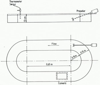
Fig. 1. A sketch of the flume used in the group C experiments conducted by Reference Tsang and HanleyTsang and Hanley (1985).
For recirculation of the water, a propeller was inserted into the flume at one end, which produced a current of about 0.15 m s−1. The flow Reynolds number during all experiments in group C was kept constant at 8.54 × 10³.
Nine different experiments were conducted in the flume. By putting the cold-room temperature at about −10°C, the water cooling rates became slightly less than 3 × 10⁻⁴ deg s−1. The water temperature was measured with a high-precision thermometer with a resolution of 0.001°C.
At different supercooling levels, the water surface was seeded by scraping a piece of ice with a saw blade. Care was taken to ensure that the same number of nuclei was planted into the water for all nine experiments. During the experiments, excellent photographs showing the time evolution of frazil-ice formation were also taken.
In analysing the data, Reference Tsang and HanleyTsang and Hanley (1985) used the integrated equation for heat conservation. By nondimensionalizing the data, several conclusions on supercooling and frazil-ice formation in sea-water were reached. Basic questions, answered by the laboratory analysis, were related to the frazil-ice morphology and the temperature evolution during freezing. In their analysis, Reference Tsang and HanleyTsang and Hanley (1985) introduced several parameters. In Table I, some of these, which will also be used in the present paper, are given. Also, in Figure 2, some parameters are clarified.

Fig. 2. Time–temperature curve during ice formation with definitions of some basic parameters. For nomenclature, see Table I.
Table I. Some Parameters Used by Reference Tsang and HanleyTsang and Hanley (1985)

In section 5, the experimental findings will be compared with calculations by the present model. First, however, the mathematical formulation and some details about the calculation will be given.
3. Mathematical Formulation
3.1. Basic assumptions
The mathematical model will restrict its attention to horizontally homogeneous flow, which means that horizontal inhomogeneities in the experiment will be neglected. It will be assumed that there is no mean vertical velocity, except for the frazil-ice rise velocity. The flow is considered to be a one-dimensional turbulent channel flow. The buoyancy effects in the flow are assumed to be caused by vertical gradients in temperature, salinity, and frazil-ice concentration.
Turbulent exchange coefficients are calculated with a kinetic energy-dissipation model of turbulence.
The initial nucleation, which was due to seeding in the experiments, is treated as a surface-boundary condition for the frazil-ice concentration equation.
The frazil-ice crystals are assumed to be thin plates of uniform size. The heat transfer between the ice crystals and the surrounding water is calculated by introducing the Nusselt number. The two phases, water and ice, are treated as one mixture phase.
The flow Reynolds number, the seeding rate, the mean size of the frazil-ice crystals, and the Nusselt number are all assumed to be constant during the calculations.
3.2 Mean flow equations
Primarily, it is the temperature and the ice concentration that are of interest but a few more variables are needed. The velocity distribution in a turbulent channel flow needs to be considered, since turbulence is produced by shear. Also, salinity is needed, as the ice crystals reject salt during ice formation.
Within the assumptions made and using a simplified water-density equation, the mean flow equations take the following form:


where z is the vertical space coordinate positive upwards, t is the time coordinate, U is the mean horizontal velocity, W c is the frazil-ice rise velocity, C i is the mean volume fraction of frazil ice, S is the mean salinity, T is the mean temperature, ρ M is the mixture density of frazil ice and sea-water, ρ I is the density of frazil ice, ρ W is the density of sea-water, ρ 0 is the reference density, T ρM is the temperature of maximum density, and α and β are constants used in the sea-water density calculation. The kinematic eddy viscosity is denoted by v T, while, σ C, σ S, and σ T are Prandtl/Schmidt numbers for frazil-ice concentration, salinity, and temperature, respectively. The mean flow is driven by a pressure gradient denoted by ∂P/∂x. The source terms, because of ice formation, are denoted by G C, G S, and G T, respectively. The mean volume fraction of frazil-ice concentrations satisfies the inequality
The convection heat transfer per unit ice area between an ice crystal and surrounding water reads:
where h is the average convection heat-transfer coefficient and T i the ice-surface temperature.
The average convection heat-transfer coefficient is calculated by introducing the Nusselt number, defined as

where l is a characteristic length and k w the thermal conductivity of sea-water.
For ice crystals growing edgewise and thus forming plates, the ice-crystal thickness (de ) is assumed to be the relevant length scale (see Fig. 3).

Fig. 3 The assumed frazil-ice crystal morphology.
The convection heat transfer for melting ice in sea-water has been studied in a series of experiments by Reference Gebhart, Gebhart, Sammakia and AudunsonGebhart and others (1983) and by Reference Samakia and GebhartSammakia and Gebhart (1983). In their analyses, experimental relationships on the Nusselt number for different melting situations can be found. The author is not aware of corresponding studies on ice formation in sea-water.
The convection heat transfer per unit ice area then reads:

The different source termas associated with frazil-ice formation can now be derived by considering a unit volume with a mixture of water and frazil ice.
The total heat gained during freezing per unit volume becomes:

where N is the total number of ice crystals in the volume V M and Ae is the mean ice-crystal area in the growing direction.
From the definition of frazil-ice concentration one can write:

where Vi is the mean ice-crystal volume.
The temperature increase during ice formation from ice crystals growing edgewise then reads:
where d f is the mean face diameter and c p is the specific heat of sea-water.
The temperature increase per unit volume corresponds directly to an ice formation of:
where L is the latent heat of ice.
Also, as salt is rejected from the crystals, the salt production reads:

where S i is the ice-crystal salinity, assumed to be zero in the present calculations.
Boundary conditions for the mean-flow equations at the surface are specified according to:


where F c is the mass exchange through the air/water interface caused by seeding, and F N is the net heat loss.
At the lower boundary, a zero-flux condition is used for all variables, except for velocity, where a zero velocity condition is given.
3.3. Turbulence model
The turbulence model is based on turbulent-exchange coefficients calculated with a two-equation model of turbulence, one equation for the turbulent kinetic energy and another for the dissipation rate of turbulent kinetic energy. The present turbulence model is the same as the one used by Reference Omstedt and SvenssonOmstedt and Svensson (1984). The equation reads:


where k is the turbulent kinetic energy and ϵ is its dissipation rate, P s is production rate due to shear, and P b is production/destruction due to buoyancy; C µ, C 1ϵ, C 2ϵ and C 3ϵ are constants used in the turbulence model (see Table II).
Table II. Constants in the Turbulence Model

Boundary conditions used in the turbulence model are that the turbulent kinetic energy and its dissipation rate are related to the friction velocity and the heat loss at the surface, and that zero-flux conditions are assumed at the bottom.
3.4. Consideration of applicability
The purpose of the present study is to analyse the laboratory experiments conducted by Reference Tsang and HanleyTsang and Hanley (1985) in relation to the mathematical model given above. First, the applicability of the model is considered.
In the race-track-shaped flume, the water was recirculated and cooled through the air/water interface. This implies that a one-dimensional approach should be suitable for the mathematical formulation of the experiments.
Turbulence was generated partly by a propeller inserted into the flume at one end and partly by bottom- and side-wall effects. Also, because the flume was curved, secondary circulation was probably present in the experiments. The mathematical model treats the flume as a turbulent channel flow, using a turbulence model, which is well established for this kind of flow (see Reference RodiRodi, 1980).
In a turbulent channel flow, the flow is driven by a pressure gradient and mixed because of current shear at the water/bottom interface. As the propeller, the side-wall effect, and the geometry all work to change and increase the turbulence level in the experiments, it was decided to test how sensitive the solutions were for different flow Reynolds numbers. This too will be discussed in section 6.2.
The initial nucleation in the experiments was caused by seeding the supercooled water with ice crystals. This model treats the seeding as a boundary condition for the frazil-ice concentration. The initial condition for the frazil ice is zero ice concentration, which implies that frazil ice can only start to increase in the calculations because of the boundary condition.
From the experimental data, it was observed that saline frazil ice formed crystals of two basic shapes: a twodimensional Christmas-star shape and a three-dimensional thorn-ball shape. From photographs taken during these experiments, made available to the present author, one can notice that the two-dimensional crystal shape dominates. In the model, the crystal structure is therefore approximated as a two-dimensional uniform plate.
These considerations indicate that the mathematical model is well suited to the experimental situation. Details about the frazil-ice growth, multiplication, break-up, and flocculation are not treated in the present formulation.
4. Details of Calculations
Equations (1)–(10) and (15)–(19) form a closed system. The equations, in their finite difference form, were integrated forward in time using an implicit scheme and a standard tri-diagonal matrix algorithm (Svensson, 1984). The equations were solved for all the nine experiments in group C conducted by Reference Tsang and HanleyTsang and Hanley (1985), using input data according to Tables III and IV.
Table III. Experimental Data

Table IV. Model Constants used in Present Calculation

The rise velocity, within the Stokes range, for a mean frazil-ice crystal size according to Table IV and with a resistance factor of 1.7, is calculated as 5 × 10⁻³ m s−1 (see Reference Ashton and MeyerAshton, 1983). This is, however, an overestimate, since turbulence influences the drag and increases the resistance factor (see Reference GrafGraf, 1971). The rise velocity is therefore somewhat reduced in Table IV.
The initial conditions were given as zero velocity, −1.5°C temperature, no ice crystals, and 30‰ salinity.
For each experiment the calculation procedure was as follows. The pressure gradient was first iterated until it converged, which was achieved with 200 time steps. Next, the net heat loss, F N, was added, giving a cooling rate in accordance with the specific experiment. At a given amount of supercooling, the mass exchange, F C, was added and after four time steps switched off, giving about 1000 ice crystals in the water. After that the calculations were continued to the desired frazil-ice concentration.
The numerical solutions were tested and found to be grid and time-step independent. This was achieved with 20 grid cells covering a depth of 0.11 m and with a time step, which was chosen as 30 s for cooling down to the seeding temperature and as 1 s for further calculations. For comparison with the experimental data, the results were integrated vertically.
5. Results
5.1 Introduction
The results are presented in this section. First, calculations of some characteristic parameters are compared with the experimental data. Secondly, the average rate of frazil-ice production is treated. Finally, the time evolutions for frazil-ice formation are analysed, based on calculations and measurements. The nomenclature follows that of Reference Tsang and HanleyTsang and Hanley (1985) (see Table I and Fig. 2).
It should also be noted that the experimental data are represented by solid lines in Figures 4–7, Reference Tsang and HanleyTsang and Hanley (1985) obtained these curves by fitting the data, using the least-squares method, to different experimental relationships. For a discussion about the accuracy of the experimental data and also how well the data were represented by the different experimental relationships, the reader is referred to Reference Tsang and HanleyTsang and Hanley (1985).

Fig. 4 Measured and calculated relationship between the characteristic lime. tc, and the amount of supercooling at seeding, ΔTn.

Fig. 7 Measured and calculated relationship between the average rate of frazil-ice production.
5.2 Characteristic parameters
Reference Tsang and HanleyTsang and Hanley (1985) characterized the data by the supercooling amount at seeding (ΔT n), the maximum supercooling (ΔT min), the characteristic time (tc ), and the characteristic ice concentration
In Figure 4 the experimental relationship found by Reference Tsang and HanleyTsang and Hanley (1985) between tc and ΔT n is compared with calculated values according to the present model. The experimental relationship is based on data from all salinity experiments in groups A, B, and C. The good agreement between the experimental findings and the present calculations was achieved by assuming a mean face diameter, a mean thickness, and a mean Nusselt number of 10−3 m, 10−4 m, and 4, respectively. From inspection of the photographs taken during the experiments, this mean size of the frazil ice seems to be in reasonable accordance with the experimental data. It should be noted that the mean values represent both time and space averages during the ice formation.
From theoretical considerations, Reference DalyDaly (1984) proposed a Nusselt number formulation for fresh water. In that formulation, the Nusselt number was related to a non-dimensional crystal size, defined as the ratio between the ice-crystal radius and the Kolmogorov length scale of turbulence.
In the present calculations, based on a flow Reynolds number of 8.54 × 10³, the non-dimensional crystal size becomes 0.6. Using this value and observing that the Nusselt number in the present study is based on the whole ice thickness, Reference DalyDaly (1984) predicted a slightly higher Nusselt number than the present one. For turbulent flow at higher Reynolds numbers, which is most likely to be the case in the experiments, the non-dimensional crystal size increases and the Nusselt number decreases.
In Figure 5 the experimental relationship found by Reference Tsang and HanleyTsang and Hanley (1985) between

Fig. 5 Measured and calculated relationship between the characteristic frazil-ice concentration by mass,
In Figure 6 the experimental relationship found by Reference Tsang and HanleyTsang and Hanley (1985) between ΔT min and ΔT n is compared with calculated values according to the present model. The agreement is excellent, except there is a slight discrepancy at zero ΔT n. The calculations illustrate that a small amount of supercooling is needed before ice starts to form. This can also be found in the laboratory data.
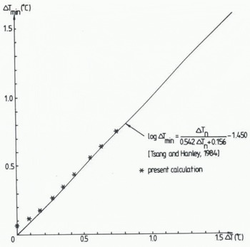
Fig. 6 Measured and calculated relationship between the temperature at maximum supercooling. ΔTmin, and the amount of supercooling at seeding, ΔTn.
5.3 Average rate of frazil-ice production
The average rate of frazil-ice production


For nomenclature see Table I.
In Figure 7, the experimental relationship found by Reference Tsang and HanleyTsang and Hanley (1985) between

5.4 Normalized parameters
The time evolution during frazil-ice formation is studied by non-dimensionalizing the data.
In Figure 8 the data from all nine experiments in group C are plotted against calculations according to the present model. It should be noted that the solid lines now represent the calculated values while the experimental data are given by different symbols.
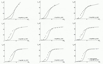
Fig. 8 Measured and calculated relationship between the normalised frazil-ice concentration
From this figure one can observe that the calculations reproduce the data quite well, except for small values of the normalized time. This is due to the fact that a constant mean size is used in the calculations. In the experiments one could easily observe how the crystals grew. The discrepancy in Figure 8 is therefore attributed to the growth of the very first small crystals, which probably heated the surrounding water more effectively compared with the larger ones.
Reference Tsang and HanleyTsang and Hanley (1985) condensed all experimental data from groups A, B, and C into one average curve for the normalized concentration as a function of the normalized time. The scatter of the data from that average curve was considered to be due to experimental uncertainty. The accuracy of the experimental data in Figure 8 was discussed further by Reference Tsang and HanleyTsang and Hanley (1985) but no statistical interpretation was given because of the rather small number of experiments.
6. Discussion
6.1. Introduction
In this section some further details and implications from the calculations are given. First, the sensitivity of the mean flow parameters are tested against turbulent intensity. Secondly, some vertical profiles of frazil-ice concentration and turbulent viscosity are discussed. Finally, the normalized rate of frazil-ice production is used as a tracer on frazil-ice dynamics.
6.2. Turbulent mixing
In the experiments, additional mixing effects (propeller, side walls, and geometry) were introduced compared with a turbulent channel flow. Turbulent mixing was therefore probably increased. To test how sensitive the mean flow parameters were to increased mixing, the flow Reynolds number was increased by factors of 2 and 10. In the sensitivity test it was found that the vertically integrated mean flow parameters did not change, within the tested Reynolds number range. However, the calculated values of the Kolmogorov length scale of turbulence decreased. The implication of this effect on the Nusselt number was discussed in section 5.2.
6.3. Damping
In the present model there is a strong interaction between ice formation and the hydrodynamics of the boundary layer. Stratification effects in the model are caused by vertical gradients in temperature, salinity, and frazil-ice concentration. During ice formation the ice concentration soon dominates, damping the turbulence due to a stable stratification.
From the photographs taken during the experiments, one could easily observe how the frazil ice was initially suspended in the flume, but, as ice formation proceeded, the frazil-ice concentration became more and more stratified with less tendency for mixing.
In Figure 9 some vertical profiles from the present model are given. The plots are taken from calculations simulating experiment number 9 in group C and they illustrate how the dynamical eddy viscosity is damped due to an increased frazil-ice concentration. The calculated profiles seem to be in good qualitative agreement with the experimental ones.
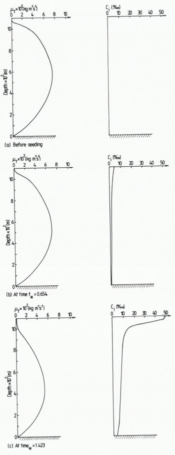
Fig. 9 Calculated vertical distribution of the frazil-ice concentration Ci and the dynamical eddy viscosity µT. Calculations according to group C, experiment number 9.
6.4. Frazil-ice dynamics
Reference DalyDaly (1984) stated that “frazil-ice dynamics” describe the unique internal feed-back loop that regulates the crystal-size distribution. In this section we shall follow Reference Tsang and HanleyTsang and Hanley (1985) and discuss the normalized rate of frazil-ice production as a tracer of the frazil-ice dynamics.
From the experiments by Reference Tsang and HanleyTsang and Hanley (1985) it was found that the normalized rate of frazil-ice production

Reference Tsang and HanleyTsang and Hanley (1985) claimed that a single-peaked bell-shaped curve was a tracer of discoid frazil-ice crystals. The double-peaked production curves were due to the formation of two types of frazil-ice crystals, the Christmas-star-shaped and the thorn-ball-shaped ones.
In Figure 10 the calculated values of

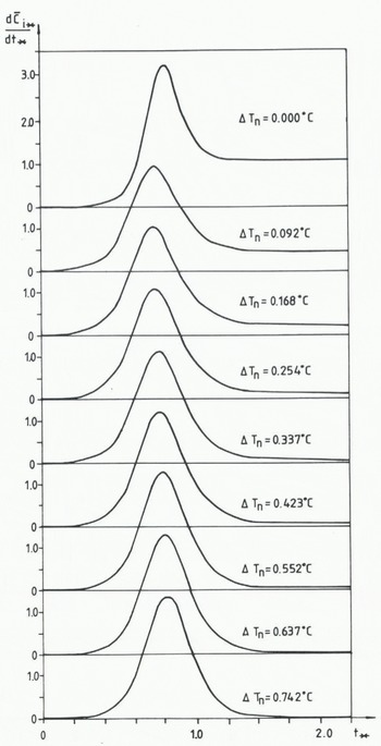
Fig. 10 Calculation relationship between the normalized rate of frazil-ice production.

In modelling double or triple peaks, some more basic shapes have to be introduced into the mathematical formulation. Also, knowledge about how the different crystals grow and interact is required. This is, however, probably far from the present knowledge.
7. Summary and Conclusions
The objective of this study has been to examine supercooling and frazil-ice formation in sea-water. For this purpose, laboratory measurements conducted by Reference Tsang and HanleyTsang and Hanley (1985) were compared with calculations from a modified version of the mathematical model presented by Reference Omstedt and SvenssonOmstedt and Svensson (1984).
The experiments were conducted in a Plexiglass flume of race-track shape, filled with sea-water, recirculated by a propeller, and placed in a cold room. The mathematical model was based on a turbulent channel-flow boundary-layer theory, in which buoyancy effects became important because of vertical gradients in frazil-ice concentration, salinity, and temperature. The initial nucleation was due to seeding and the frazil-ice crystals were treated as thin uniform plates.
The general experimental findings were most satisfactorily reproduced by the model, giving confidence to the mathematical formulation. The mathematical model can thus serve as a good base for further studies on frazil-ice dynamics.
Acknowledgement
This work is a part of the Swedish–Finnish Winter Navigation Research Programme and has been financed by the Swedish Administration of Shipping and Navigation. I should like to thank L. Funkqvist, L. Nyberg, and U. Svensson for valuable comments on an earlier version of the present paper and also Dr G. Tsang for his kind assistance during my stay at the Canada Centre for Inland Waters.


