


1. Introduction
Viscoelastic fluids exhibit both viscous and elastic behaviour owing to a microstructural component that responds elastically under strain, thus imparting an elastic response in addition to the viscous response. This class of fluids is commonly encountered in biological (e.g. blood and mucus) and industrial (e.g. polymer processing and surfactants) flows. Taking a polymer solution as a representative viscoelastic fluid, as the polymer chains advect over curved streamlines, they can accumulate stress while being elongated, and dissipate that stress over a characteristic time scale  $\lambda$ while recoiling. A measure of the contribution of the elastic effect is the Weissenberg number (
 $Wi =\lambda \dot {\gamma }$, where
  $\dot {\gamma }$ is the shear rate). Beyond a critical
  $Wi_{c}$, accumulated elastic stress has been observed to drive purely elastic flow instabilities on curvilinear streamlines (McKinley, Pakdel & Öztekin Reference McKinley, Pakdel and Öztekin1996; Pakdel & McKinley Reference Pakdel and McKinley1996) despite negligible inertial effects; while at small Reynolds number
  $Re \ll 1$, Newtonian fluids would remain laminar and stable. The Pakdel–McKinley criterion has been used to capture effectively the onset of the elastic instability when the parameter
  $M = \sqrt {2\,Wi\,\lambda U/R}$ surpasses a critical
  $M_{c}$ dependent on the flow geometry and fluid rheology (McKinley et al. Reference McKinley, Pakdel and Öztekin1996; Pakdel & McKinley Reference Pakdel and McKinley1996). The
  $M$ parameter relates flow field perturbations and elastic stresses as a perturbation scale
  $\lambda U/R$ from the average flow velocity
  $U$ and streamline radius of curvature
  $R$, and takes
  $Wi$ as the strength of elastic tensile stresses. Thus a critical
  $M_{c}$ must be surpassed for an elastic instability to propagate in an arbitrary flow. The
  $M$ parameter has been shown to generalize the critical conditions for elastic stress buildup for a broad spectrum of flow geometries spanning microscopic to macroscopic scales, with a typical transition point of approximately
  $M_{c} = 1\unicode{x2013}7$ (McKinley et al. Reference McKinley, Pakdel and Öztekin1996; Morozov & van Saarloos Reference Morozov and van Saarloos2007; Zilz et al. Reference Zilz, Poole, Alves, Bartolo, Levaché and Lindner2012; Haward, McKinley & Shen Reference Haward, McKinley and Shen2016; Qin et al. Reference Qin, Salipante, Hudson and Arratia2019; Kumar & Ardekani Reference Kumar and Ardekani2021).
At high  $Wi \gg 1$ and low
  $Re \ll 1$, a chaotic elastic flow instability can arise bearing qualitative similarities to inertial turbulence (IT), thus termed elastic turbulence (ET). Both IT and ET exhibit substantial increases in flow resistance and mixing rate compared to their corresponding laminar regimes, and are comprised of a broad range of spatiotemporal modes with a spectral power-law decay exponent
  $\alpha$ (Groisman & Steinberg Reference Groisman and Steinberg2000, Reference Groisman and Steinberg2001; see review article Steinberg Reference Steinberg2021). For ET, various studies have reported a steep
  $\alpha \approx 3.5$, with sensitivity to the specific flow geometry (Steinberg Reference Steinberg2021). ET is thus temporally chaotic but spatially smooth, with dominance of a few low-order, vessel-scale modes, similar to IT flow on scales below the dissipation scale, viz. the Batchelor regime (Batchelor Reference Batchelor1959; Burghelea, Segre & Steinberg Reference Burghelea, Segre and Steinberg2005; Steinberg Reference Steinberg2021). These characteristics lend utility to ET, and numerous industrial and environmental processes have been proposed that leverage the ET flow of polymer solutions through porous media for a spectrum of applications such as enhanced oil recovery (EOR), filtration, or groundwater remediation (Clarke et al. Reference Clarke, Howe, Mitchell, Staniland, Hawkes and Leeper2015; Howe, Clarke & Giernalczyk Reference Howe, Clarke and Giernalczyk2015). ET is driven by elastic stress reacting on the flow field, which is inherently difficult to quantify in situ. Furthermore, the spatiotemporal nature of ET means that a complete evaluation would be supported by the quantification of three-dimensional (3-D) flow fields spanning several vessel scales over long time scales. ET has been characterized in three dimensions primarily via direct numerical simulations for flows such as Taylor–Couette flow (Thomas, Sureshkumar & Khomami Reference Thomas, Sureshkumar and Khomami2006; Thomas, Khomami & Sureshkumar Reference Thomas, Khomami and Sureshkumar2009) and von Kármán swirling flow (Khambhampati & Handler Reference Khambhampati and Handler2020; van Buel & Stark Reference van Buel and Stark2022). Experiments have used holographic particle tracking to probe aspects of ET in three dimensions, such as particle dispersion (Afik & Steinberg Reference Afik and Steinberg2017), while ET flow fields have been assessed about a 3-D cross-channel via particle tracking velocimetry and supported by pressure measurements (Qin et al. Reference Qin, Ran, Salipante, Hudson and Arratia2020). However, a volumetric quantification of ET near zero
  $Re$ evolving over a broad spatial scale (numerous vessel scales) remains lacking.
Regarding porous media flow in general, whereas viscous flow through porous media mixes poorly at the micro-scale due to the low  $Re$, the elastic contribution provided by polymer stretching enhances the mixing in each pore and the overall dispersion of flow through the medium (Scholz et al. Reference Scholz, Wirner, Gomez-Solano and Bechinger2014). For shear-thinning solutions in this context, viscoelastic effects lead to a seemingly paradoxical pressure increase from the flow for increasing flow rates, despite the accompanying shear-thinning behaviour of the bulk solution (Marshall & Metzner Reference Marshall and Metzner1967; Durst, Haas & Kaczmar Reference Durst, Haas and Kaczmar1981). Clarke et al. (Reference Clarke, Howe, Mitchell, Staniland and Hawkes2016) demonstrated that the viscoelastic effect in question was likely caused by elastic turbulence, supporting earlier observations in situ by Mitchell et al. (Reference Mitchell, Lyons, Howe and Clarke2016), and further validated the efficacy of ET for EOR. Recently, Browne & Datta (Reference Browne and Datta2021) were able to deduce an energy balance to relate directly the energy dissipation of a random porous medium to the pore-scale flow fluctuations of ET above
  $Wi_{c} = 2$. However, they noted that the energy balance neglected extensional viscosity and strain history effects, and that these effects likely became significant for
  $Wi > 4$ where the energy balance underpredicted the losses observed from experiments.
In a prior work, Browne, Shih & Datta (Reference Browne, Shih and Datta2020a) investigated viscoelastic flow through one-dimensional (1-D) model porous media for a system scale ranging from a single pore up to a thirty-pore sequence. Their experiments highlighted the importance of spatial correlation. Whereas flow above  $Wi_{c}$ through a single pore generates an upstream vortex typical of a viscoelastic contraction flow instability (McKinley et al. Reference McKinley, Raiford, Brown and Armstrong1991; Rothstein & McKinley Reference Rothstein and McKinley1999; Carlson, Shen & Haward Reference Carlson, Shen and Haward2021), the presence of sequential pores results in a reduced
  $Wi_{c}$ and the occurrence of bistable states of laminar and unstable flow. Flow through pores under a laminar state exhibits a corner vortex, while unstable flow is typified by strongly fluctuating streamlines flooding the corners of the pore. They hypothesized that the flow states were driven by competition between the extension and relaxation of polymer chains as they advected through the array. This notion was supported by later numerical work by Kumar et al. (Reference Kumar, Aramideh, Browne, Datta and Ardekani2021). For closely placed pores in a 1-D array, Kumar et al. showed that the laminar flow through pores with eddy-dominated flow was accompanied by increased polymeric stress (extended polymer chains), whereas unstable flow through thus eddy-free pores exhibited reduced stress (coiled polymer chains).
Of relevance to these findings is the time scale ratio for which they manifest. Within the context of repeating pores, the pertinent time scales can be related as a pitch-based Deborah number, generally defined as  $De = U\lambda / L$, where
  $L/U$ provides a time scale for material advection between pores separated by distance
  $L$. For
  $De > 1$, microstructures are advected between pores faster than they can relax. Kumar et al. (Reference Kumar, Aramideh, Browne, Datta and Ardekani2021) noted that the flow instability for a ten-pore sequence started at
  $Wi > 18$ and
  $De > 1$: pore interaction affects the onset of instability for sufficiently large arrays. A later work reported a similar onset with
  $De$ for an instability occurring between two cylinders (Kumar & Ardekani Reference Kumar and Ardekani2021), and experiments by Ekanem et al. (Reference Ekanem, Berg, De, Fadili and Luckham2022) found that increased
  $De$ lowers
  $M_{c}$ for flow instability about separated pores. Indeed, the significance of
  $De$ for flow instability in repeating arrays was shown in experiments by De et al. (Reference De, Van Der Schaaf, Deen, Kuipers, Peters and Padding2017) for a two-dimensional (2-D) ordered array of cylinders. They found coexisting lanes of fast and slow flow in the array above
  $De = 1.5$, leading to flow crossing between channels driven by strong crossflow action. They conclude that
  $De$ is more apt than
  $Wi$ to indicate large-scale instabilities in repeating arrays. Walkama, Waisbord & Guasto (Reference Walkama, Waisbord and Guasto2020) and Haward, Hopkins & Shen (Reference Haward, Hopkins and Shen2021) considered viscoelastic flow through ordered and increasingly disordered cylinder arrays, and both works show that ET is likely controlled by the concentration of stagnation points in 2-D arrays. This is an analogous explanation for the
  $De$ scaling by De et al. (Reference De, Van Der Schaaf, Deen, Kuipers, Peters and Padding2017), where they in effect also modulated the concentration of stagnation points while geometrically scaling cylinder spacing for different
  $De$.
$De$.
Experiments for viscoelastic flow through porous media encounter common limitations: the media are typically opaque, and flow is spatiotemporally sensitive to the specific geometric configuration of the medium (Walkama et al. Reference Walkama, Waisbord and Guasto2020; Haward et al. Reference Haward, Hopkins and Shen2021; Browne & Datta Reference Browne and Datta2021; with reviews by Browne, Shih & Datta Reference Browne, Shih and Datta2020b; Kumar, Guasto & Ardekani Reference Kumar, Guasto and Ardekani2022). Refractive index matching (RIM) such that the medium and flow are transparent permits direct optical access for image-based interrogation techniques. Such methods include streak imagery and particle image velocimetry (PIV) for 2-D quantification, while recent works probed 3-D flows via particle tracking velocimetry (PTV) (Holzner et al. Reference Holzner, Morales, Willmann and Dentz2015; Souzy et al. Reference Souzy, Lhuissier, Méheust, Le Borgne and Metzger2020) and tomographic PIV (TPIV) (Larsson, Lundström & Lycksam Reference Larsson, Lundström and Lycksam2018; Forslund et al. Reference Forslund, Larsson, Lycksam, Hellström and Lundström2021). Souzy et al. (Reference Souzy, Lhuissier, Méheust, Le Borgne and Metzger2020) used scanning PTV to resolve Newtonian creeping flow through randomly packed spheres (2 mm in diameter), achieving a fine spatial resolution for a time-averaged grid to show that 3-D mixing results in Lagrangian chaos for material advection. This result expanded upon prior numerical works (Turuban et al. Reference Turuban, Lester, Le Borgne and Méheust2018, Reference Turuban, Lester, Heyman, Le Borgne and Méheust2019) that showed similarly enhanced mixing for flow past a body-centred cubic array of spheres compared to a simple cubic array.
For TPIV, synchronized cameras image a region of interest (ROI) from different lines of sight (LOS) and reconstruct the position of seeded particles within a volume of interest (VOI) for local cross-correlation in time to yield a velocity field. Applied for micro-scale, a stereo microscope provides limited optical LOS such that  $\mathrm {\mu }$-TPIV can be conducted: recently, we have shown this approach to be useful for capturing transient viscoelastic flow instability in three dimensions (Carlson et al. Reference Carlson, Shen and Haward2021). While we do not match the spatial resolution of scanning PTV,
  $\mathrm {\mu }$-TPIV can time-resolve flow, which is crucial for quantifying the unsteady volumetric velocity fluctuations of ET.
In the present work, we apply  $\mathrm {\mu }$-TPIV to the study of ET in a micro-scale ordered 3-D porous medium. Besides the applied virtues for studying viscoelastic flow through porous media, we can probe a variety of length scales by imaging simultaneously multiple pores and throats across a constant focal plane, thereby accessing the flow history between pores. Thus this configuration enables a more fundamental study of the spatiotemporal evolution of ET, where due to the dominance of vessel-scale (i.e. pore-scale) modes, ET flow will appear spatially smooth at a given pore for a temporal instant. The desired geometry is therefore a geometrically ordered fully 3-D array of cubicly packed glass spheres – a hitherto unstudied configuration, with fabrication made possible via selective laser etching (Gottmann, Hermans & Ortmann Reference Gottmann, Hermans and Ortmann2012; Meineke et al. Reference Meineke, Hermans, Klos, Lenenbach and Noll2016; Burshtein et al. Reference Burshtein, Chan, Toda-Peters, Shen and Haward2019). We utilize
  $\mathrm {\mu }$-TPIV via RIM to assess flow through this novel 3-D ordered porous medium, together with pressure measurements, to provide a spatiotemporally complete quantification of ET.
From these experiments we scale the transition from laminar, to elastically unstable, to ET flow against the  $M$ parameter, showing via localized (
 $M_{L}$) calculation over pore-scale instantaneous streamlines that coexisting regions of unstable and laminar flow hold locally consistent with the
  $M$ instability criterion. In the ET state, which we validated via comparison against common spectral characteristics, we relate the seemingly disparate coexisting states of laminar and unstable flow as a continuous progression between the two that comprises the core velocity fluctuations of ET. Finally, we relate inversely correlated flow states via competing streamline curvature, and the spatial evolution between states, as positive feedback between flow resistance and upstream streamline curvature.
2. Experimental methods
2.1. Flow cell and refractive index matching
The test cell was designed to confine flow about a  $70 \times 5 \times 5$ array of
  $500\,{\mathrm {\mu }}{\rm m}$ diameter cubicly packed solid spheres (spaced
  $w_p = 500\,{\mathrm {\mu }}{\rm m}$) placed in a square-sectioned channel of width
  $w_c = 2.5\,\mathrm {mm}$, yielding nominal porosity
  $\phi = 0.4675$. The array nature of the geometry permits a simultaneous study of numerous pores at a given focal plane, and due to the constant
  $De$ throughout the array, we can assess the local flow history from time-resolved measurements. To fabricate this system, we used selective laser-induced etching (SLE) of an open-faced slab of fused silica (
 ${\rm SiO}_2$) (Gottmann et al. Reference Gottmann, Hermans and Ortmann2012; Meineke et al. Reference Meineke, Hermans, Klos, Lenenbach and Noll2016; Burshtein et al. Reference Burshtein, Chan, Toda-Peters, Shen and Haward2019) on a commercial LightFab SLE printer (LightFab GmbH, Germany), followed by chemical etching in potassium hydroxide to remove unwanted material. The open-faced flow cell was subsequently sealed with glass slides about the
  $z$ direction. As manufactured, the spheres are slightly over-etched and remain connected by glass ‘necks’ (images in figure 1a). To incorporate the actual sphere contacts in a stereolithography (STL) surface for
  $\mathrm {\mu }$-TPIV masking, we used X-ray microtomography (
 $\mathrm {\mu }$-CT; Pimenta et al. Reference Pimenta, Toda-Peters, Shen, Alves and Haward2020) to quantify precisely the surface of the geometry (shown in figure 1b). Flow was driven through the device with a volumetric flow rate
  $Q$ via two syringe pumps (neMESYS, Cetoni GmbH, Germany) in a push–pull configuration, with a wet/wet differential pressure transducer (OMEGA, USA) spanning the inlet and outlet (
 $p_1$,
  $p_2$ in figure 1c) sampling at 100 Hz. The characteristic velocity of flow passing about the array of spheres is
  $U_{p} = Q/A\phi$, the average flow velocity in each pore between spheres for a volumetric rate
  $Q$, total cell cross-sectional area
  $A = w_{c}^2$, and porosity
  $\phi$.
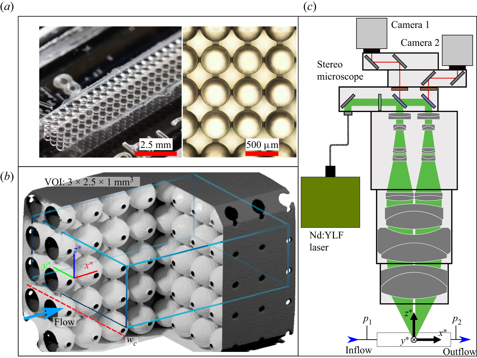
Figure 1. (a) Images of the model porous medium as manufactured and filled with water for contrast.(b) A section of the micro-CT of the porous array together with the alignment of the volume of interest (VOI, blue), centred 35 pores into the array. The fluid–solid interface is coloured white. (c) The beam path of the LaVision FlowMaster  $\mathrm {\mu }$-TPIV system.
We image the very midpoint of the array considering a VOI shown in figure 1(b) with the coordinate system triad. Views in three dimensions reference the coloured triad for orientation. For optical access through multiple fluid–solid interfaces throughout the depth of the array, we used RIM between the fluid and solid following a scheme similar to that in Larsson et al. (Reference Larsson, Lundström and Lycksam2018). A continuous 5 mW green laser was passed through the fluid-filled array onto a target 1 m away in a 25  $^\circ$C environment, and the diameter of the distorted beam for different concentrations of glycerol in deionized water was measured. In our configuration, this approach could detect a refractive index (RI) disparity of
  $10^{-4}$. We obtained a minimum distortion and thus achieved RIM at 89.5 wt% glycerol. A viscoelastic solution was prepared consisting of 130 parts-per-million partially hydrolyzed polyacrylamide (HPAA,
  $M_W = 18$ MDa, Polysciences Inc., USA), in the RI-matched solvent. For
  $\mathrm {\mu }$-TPIV measurement purposes, the fluid was seeded with
  $2\,{\mathrm {\mu }}{\rm m}$ fluorescent particles (excitation/emission 530 nm/607 nm, PS-FluoRed-Particles, Microparticles GmbH, Germany) to a particle concentration of approximately 0.03 particles per pixel at the desired magnification. Ultimately, the RI of the fluid was measured with an Anton-Paar Abbemat MW refractometer operating at 589 nm, yielding RI 1.4582 at 25
  $^\circ$C. This is in good agreement with the nominal RI 1.4584 for
  ${\rm SiO}_2$ at 589 nm (Malitson Reference Malitson1965). Although the refractometer operates at a narrow selection of wavelengths, both materials exhibit normal chromatic dispersion, and the RIM errors incurred from imaging at other wavelengths will partially cancel out (Larsson et al. Reference Larsson, Lundström and Lycksam2018).
We characterized the shear-rate dependent viscosity and extensional flow characteristics of the HPAA solution using an Anton-Paar MCR stress-controlled rheometer and a Haake capillary breakup extensional rheometer (CaBER), respectively. The fluid is weakly shear-thinning with zero shear viscosity  $\eta _0 = 500$ mPa s (figure 2a), and we take a subset of the shear rheology sweep at moderate
  $\dot {\gamma }$ to fit power-law extrapolations for the first normal stress difference
  $N_1$ and shear stress
  $\sigma$ (figure 2b) to evaluate a local
  $Wi_{L} = N_{1}(\dot {\gamma }_{L})/2\sigma (\dot {\gamma }_{L})$ discussed in § 3. Considering the extensional rheology, the fluid is viscoelastic with relaxation time
  $\lambda = 1.2$ s (figure 2c), and is strongly strain-hardening with
  $\eta _{E,app} \approx 340\eta _{0}$ at high strains (figure 2d). Here, the accumulated Hencky strain is
  $\epsilon _H = 2\ln (d_{0}/d(t))$, with the measured filament diameter
  $d$, and the initial filament diameter
  $d_0 = 6$ mm. For flow within the porous medium, the zero shear viscosity
  $\eta _{0}$ and length scale
  $w_p/2$ are used to calculate
  $Re = \rho U_{p}w_{p}/2\eta _{0}$ and the characteristic shear rate
  $\dot {\gamma } = 2U_{p}/w_{p}$ for
  $Wi = \lambda \dot {\gamma } = 2\lambda U_{p}/w_{p}$. The Reynolds number
  $Re \lesssim 10^{-3}$ is considered negligible in the present work. As the array of spheres is cubicly packed, the relevant length scale
  $L$ for a pitch-based Deborah number is
  $w_{p}$, thus in the present work,
 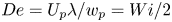 $De = U_{p}\lambda /w_{p} = Wi / 2$.
Figure 2. (a,b) Shear rheology of the HPAA solution, where (b) is at a moderate  $\dot {\gamma }$ subset of (a) to fit power-law interpolations for
  $N_1$ and
  $\sigma$. (c,d) Extensional rheology of the elastocapillary response for the relaxation time
  $\lambda$ and strain hardening response.
2.2. Microtomographic PIV ( $\mathrm {\mu }$-TPIV)

Tomographic particle image velocimetry (TPIV) is a volumetric flow measurement whereby for a particle-laden flow, numerous camera angles are used to reconstruct a particle volume that is then locally cross-correlated in time to resolve the velocity vector  $\boldsymbol {u}$ on a 3-D grid (Elsinga et al. Reference Elsinga, Scarano, Wieneke and van Oudheusden2006a). It is possible to conduct TPIV at micro-scale (
 $\mathrm {\mu }$-TPIV) via imaging from the dual LOS afforded by a stereo microscope (see Carlson et al. Reference Carlson, Shen and Haward2021). Flow was captured by a LaVision FlowMaster
  $\mathrm {\mu }$-TPIV system in a 25
  $^\circ$C environment as time-resolved recordings from dual high-speed cameras (Phantom VEO 410,
  $1280\times 800$ pixels) at a velocity-dependent frame rate spanning 25–250 Hz such that no particle moved more than 8 pixels between frames when illuminated by a coaxial Nd:YLF laser (527 nm wavelength). Images were pre-processed with an ROI mask spanning 7–5 spheres in
  $x$–
$x$– $y$ and filtered with local background subtraction and Gaussian smoothing at
  $3 \times 3$ pixels. Three-dimensional calibration was achieved by capturing images of a micro-grid in air at the planes
  $z_{air} = \pm 500$ and
  $0\,\mathrm {\mu }$m, and mapping the coordinate
  $z_{air}$ elevation to an equivalent position
  $z$ in the working fluid due to the RI change. A preliminary coordinate system was achieved by interpolating a third-order polynomial between the calibration planes. The final coordinate system was reached via volumetric self-calibration (Wieneke Reference Wieneke2008) of the pre-processed images, which distorts the original grid using the actual particle images to create a refined calibration. By iterating volume self-calibration, we reached a typical maximum disparity of 0.02 voxels. Particle reconstruction was achieved using the Fast MART (multiplicative algebraic reconstruction technique) algorithm implemented in the commercial PIV software DaVis 10.2.1 (LaVision GmbH). This algorithm creates an initial particle volume using multiplicative line of sight (Worth & Nickels Reference Worth and Nickels2008; Atkinson & Soria Reference Atkinson and Soria2009) followed by iterations of Sequential MART (Atkinson & Soria Reference Atkinson and Soria2009), then sequential motion tracking enhancement (SMTE) for ‘ghost’ suppression (Novara, Batenburg & Scarano Reference Novara, Batenburg and Scarano2010; Lynch & Scarano Reference Lynch and Scarano2015), where spurious ghost particles arise from randomly overlapping LOS and contaminate the cross-correlation (Elsinga, Van Oudheusden & Scarano Reference Elsinga, Van Oudheusden and Scarano2006b). For the present work, we determined that eight iterations of Fast MART resulted in a suitable compromise between vector quality and computation time (6 CPU-minutes per tomogram VOI,
  $T$), and observed that SMTE converged ghost intensity after a temporal march over 30 volumes. Before temporal cross-correlation, we applied the 3-D masking procedure described below to eliminate the solid region in the reconstruction.
2.3. Tomogram masking
Masking protocols for TPIV range from simple ROI projection to more sophisticated backward projection algorithms such as the visual hull approach (Adhikari & Longmire Reference Adhikari and Longmire2012), but such methods are inapplicable when the RI-matched solid is transparent and the 3-D array has highly overlapping LOS in the back-projection. Therefore we developed an alternative procedure by volume masking directly from the  $\mathrm {\mu }$-CT geometry. First, we generate a manifold of the
  $\mathrm {\mu }$-CT STL about the VOI via a solid Boolean operation in the 3-D modelling software Blender (Blender Online Community 2018), referring to the surface yielded as
  $S$. Second, we time-averaged a subset of the tomogram volumes
  $T$ as
  $\bar {T}$, and further applied
  $11 \times 11 \times 11$ voxel Gaussian smoothing to generate a reference volume for mask generation. To centre and align
  $\bar {T}$ with
  $S$, we leverage the uniform spacing of the array: we project
  $S$ and
  $\bar {T}$ onto
  $x^*$–
 $z^*$ and
  $y^*$–
 $z^*$ planes, and sum about the
  $x^*$ and
  $y^*$–
 $z^*$ axes, respectively. We compare two central
  $\bar {T}$ maxima against
  $S$ minima for the
  $x^*$–
 $y^*$ axes, and directly align the maxima and minima in
  $z^*$. An example alignment is shown in figure 3. By weighting multiple minima to locate
  $S$ in
  $\bar {T}$ in
  $x^*$–
 $y^*$, we obtain sub-voxel mask placement resolution in
  $x^*$–
 $y^*$ and single voxel resolution in
  $z^*$.
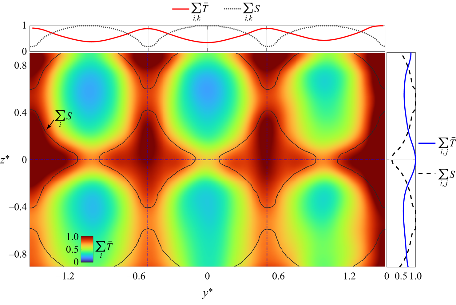
Figure 3. Example alignment between the tomogram volume  $T$ and the edges of the STL manifold
  $S$ in the
  $y^*$–
 $z^*$ plane. Here,
  $S$ and
  $T$ are projected onto the plane, then summed along
  $y^*$ and
  $z^*$.
Voxels in the de-warped mask planes of  $\bar {T}$ that were found to be inside
  $S$ via a ray-tracing algorithm are set as masked, and the planes are subsequently warped back into voxel space. We apply the mask planes in DaVis 10.2.1 to
  $T$ before multi-grid iterative cross-correlation with a final window of
  $32 \times 32 \times 32$ voxels with 8 voxel steps (75 %) to calculate the velocity field
  $\boldsymbol {u}$ with components
  $u$,
$u$,  $v$ and
  $w$. Finally, we spatiotemporally filtered the vector fields with a second-order polynomial regression across neighbourhoods of
  $5 \times 5 \times 5 \times 11$ vectors (Scarano & Poelma Reference Scarano and Poelma2009; Elsinga et al. Reference Elsinga, Adrian, Van Oudheusden and Scarano2010; Schneiders, Scarano & Elsinga Reference Schneiders, Scarano and Elsinga2017). We can estimate a signal-to-noise ratio (SNR) of this approach by taking the ratio of the average
  $\bar {T}$ intensity in the fluid (particles and ghosts) and that of the mask region (ghosts and near-boundary particles). In the present work,
  ${\rm SNR} = 3.0$, indicating that our masked reconstruction is of good quality (
 ${\rm SNR} = 2.2$ without SMTE). Whereas historically, time-resolved PIV has been burdensome technically, modern approaches for TPIV are increasingly reliant on accessing time-resolved quantities such as in SMTE (Beresh Reference Beresh2021).
For a posteriori assessment of our measurement quality, we validated conservation of mass for a time-averaged vector field (Zhang, Tao & Katz Reference Zhang, Tao and Katz1997). We take flow divergence  $\boldsymbol {\nabla }\boldsymbol {\cdot }\boldsymbol {u}$ assessed relative to an assumption of incompressible flow (relative error
  $\zeta = (\boldsymbol {\nabla }\boldsymbol {\cdot }\boldsymbol {u})^2 / \mathrm {tr}(\boldsymbol {\nabla }\boldsymbol {u}\boldsymbol {\cdot }\boldsymbol {\nabla }\boldsymbol {u})$, using the trace
  $\mathrm {tr}$). At the maximum
  $Re$, the error is
  $\zeta = 0.2$ (see figure 4 for joint p.d.f.s of
  $\boldsymbol {\nabla }\boldsymbol {\cdot }\boldsymbol {u}$ components and the p.d.f. of
  $\zeta$), in good agreement with limited LOS TPIV experiments (Kempaiah et al. Reference Kempaiah, Scarano, Elsinga, van Oudheusden and Bermel2020) and our prior work (
 $\zeta = 0.25$; Carlson et al. Reference Carlson, Shen and Haward2021). In addition, a comparable
  $\zeta$ from our prior work indicates that the fluid–structure RIs are properly matched: the fluid–structure reconstruction results in a vector quality similar to that from a fluid only.

Figure 4. (a) Joint probability density functions (p.d.f.s) of the components of divergence for the solvent at  $Re = 10^{-3}$. Points away from the zero divergence plane (
 $\boldsymbol {\nabla }\boldsymbol {\cdot }\boldsymbol {u} =0$) indicate measurement error, which can be calculated as a relative divergence error parameter
  $\zeta$. (b) The p.d.f. of
  $\zeta$.
3. Results and discussion
Pressure and  $\mathrm {\mu }$-TPIV measurements were taken over a range of flow rates corresponding to
  $0.5\leq Wi \leq 8.2$ for the HPAA solution, and
  $10^{-5}\leq Re \leq 10^{-3}$ for the solvent, considering a VOI midway into the porous array (35 pores). We use the pressure data, which can be interpreted in real time, to gauge the overall flow state and limit resource-intensive
  $\mathrm {\mu }$-TPIV reconstruction to selected
  $Wi$ and
  $Re$. In discussing the flow, we non-dimensionalize the vector field
  $\boldsymbol {u}$ by the average pore velocity
  $U_{P}$, and length scales by
  $w_{p}$ (e.g.
  $\lvert \boldsymbol {u} \rvert ^*=\lvert \boldsymbol {u} \rvert /U_{p}$,
  $v^*=v/U_{p}$,
  $x^* = x/w_{p}$). From the rate-of-strain tensor
  ${{\boldsymbol{\mathsf{D}}}} = (\boldsymbol {\nabla } \boldsymbol {u}+\boldsymbol {\nabla } \boldsymbol {u}^{\rm T})/2$, we calculate the magnitude
  $|{{\boldsymbol{\mathsf{D}}}}|$ as
  $\dot {\gamma }_{L} = \sqrt {2({{\boldsymbol{\mathsf{D}}}}:{{\boldsymbol{\mathsf{D}}}})}$ and reduce it as
  $\dot {\gamma }^* = \dot {\gamma }_{L} w_p / (2 U_p)$. We introduce the common flow type parameter
  $\xi$ (Astarita Reference Astarita1979) as a map of the flow topology:
  $\xi = (|{{\boldsymbol{\mathsf{D}}}}|-|\pmb {\it \varOmega }|)/(|{{\boldsymbol{\mathsf{D}}}}|+|\pmb {\it \varOmega }|)$, where
  $\pmb {\it \varOmega }= (\boldsymbol {\nabla } \boldsymbol {u}-\boldsymbol {\nabla } \boldsymbol {u}^{\rm T})/2$ is the spin tensor. Thus
  $\xi = -1$ for flow dominated by solid body rotation,
  $\xi = 0$ for shear flow, and
  $\xi = 1$ for extensional flow.
We present the solvent flow field in figure 5 as a baseline case at the maximum  $Re$ (
 ${Wi = 0}$). Here, we show
  $x^*$–
 $y^*$ slices of
  $v^*$ and
  $\dot {\gamma }^*$ as well as numerically advected massless particles (Paraview 5.10; Ahrens, Geveci & Law Reference Ahrens, Geveci and Law2005) coloured by
  $\lvert \boldsymbol {u} \rvert ^*$ and
  $\dot {\gamma }^*$ from the background grid. A single ring of particles is injected from
  $x^* = 0$ at each time step, thus their consistent grouping indicates steady-state flow. The particle fields show fluctuating
  $\lvert \boldsymbol {u} \rvert ^*$ and
  $\dot {\gamma }^*$ as they are advected between pore throats and bodies, tracking shear flow through pore throats and extension-dominated flow about the pore bodies consisting of alternating compressional and extensional flow in each pore. Spatially, the fields of
  $v^*$ and
  $\dot {\gamma }^*$ are consistent between sequential pores, thus we determine that the VOI is sufficiently deep in the array to consider it fully developed laminar flow.

Figure 5. Instantaneous numerical particle field and  $x^*$–
 $y^*$ slice at
  $z^* = 0$ for the glycerol solvent flow at
  $Re = 10^{-3}$. The particle fields are coloured by (a)
  $\lvert \boldsymbol {u} \rvert ^*$ and (b) the flow type parameter
  $\xi$, while the slices map the crossflow velocity
  $v^*$ and rate of strain
  $\dot {\gamma }^*$, respectively.
3.1. The transition from laminar to elastically turbulent flow
Flow passing through a porous medium at low  $Wi$ and low
  $Re$ is expected to drive a pressure drop that varies approximately linearly with flow rate for the Boger fluids used in our experiments, as per Darcy's law. Thus to delineate our flow regimes, we consider the pressure drop data presented in figure 6. In figure 6(a), we show the time-averaged polymeric contribution to the pressure drop
  ${\rm \Delta} \bar {p}-{\rm \Delta} \bar {p}_{n}$ between the inlet and outlet of the microchannel. Here,
  ${\rm \Delta} p$ is the pressure drop (i.e.
  $p_1 - p_2$) measured for the flow of the polymer solution, and
  ${\rm \Delta} p_n$ is the pressure drop measured for the Newtonian solvent. Both were recorded over 180 s at each imposed volumetric flow rate
  $Q$. We see that for low
  $Wi$ (
 $0.5\leq Wi \leq 1.8$), the pressure drop obeys the laminar model (
 $r^2 = 0.99$), with a slight deviation at
  $Wi = 1.8$, but the polymeric contribution breaks this expectation at higher flow rates
  $Wi \geq 2.6$, resulting in the often discussed increased flow resistance driven by elastic effects (Marshall & Metzner Reference Marshall and Metzner1967; Durst et al. Reference Durst, Haas and Kaczmar1981; Browne & Datta Reference Browne and Datta2021). We use the departure point of the pressure drop data from the linear trend to estimate the critical
  $Wi$ as
  $Wi_{c} = 1.8$, i.e. the highest
  $Wi$ data point to fall near the trend.
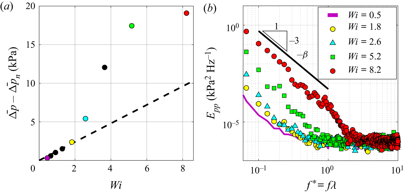
Figure 6. (a) The polymeric contribution to the pressure drop across the flow cell. (b) Power spectra  $E_{pp}$ for selected
  $Wi$ highlighting the gradual strengthening of ET for increasing
  $Wi$. The dashed line in (a) indicates a linear regression fit below
  $Wi_{c}$.
To further describe the transition from laminar to unstable flow, we present power spectra  $E_{pp}$ of the fluctuating pressure
  $p' = {\rm \Delta} p - \bar {{\rm \Delta} p}$ against dimensionless frequency
  $f^* = f\lambda$ in figure 6(b). Despite the pressure drop deviation in figure 6(a) for
  $1.8\leq Wi \leq 2.6$, when comparing the pressure power spectra of laminar flow at
  $Wi = 0.5$ to that of an apparently unstable flow at
  $Wi = 2.6$, one observes that they are quite similar, with slightly increased power in the lower
  $f^*$ for the unstable state. Evidently, the near-critical unstable flow state is weakly transient (we quantify the flow transience in the Appendix). For increasing
  $Wi$, the transient state grows in power, and by
  $Wi = 8.2$, we observe sustained increased power throughout the lower frequency range, with a steep power-law decay exponent
  $\beta \approx 3$ (which is typical of ET) up to
  $f^*=1$, i.e. the fluctuation time scale
  $1/f$ matches that of the polymer relaxation time
  $\lambda$. We hypothesize that the higher frequency roll-off towards
  $f^* = 2$ down to the noise floor is due to polydispersity of the HPAA, and generalize that
  $1/\lambda$ is a common upper bound for capturing the majority of the energy of ET (Browne & Datta Reference Browne and Datta2021). While the power spectra show that a smooth macro-scale transition towards stronger ET occurs with increasing
  $Wi$, we next consider the local micro-scale evolution.
3.2. Instability: a local curvature balance
In § 1 we introduced a common scaling parameter  $M = \sqrt {2\,Wi\,\lambda U/R}$ (McKinley et al. Reference McKinley, Pakdel and Öztekin1996; Pakdel & McKinley Reference Pakdel and McKinley1996) as a generalized predictor for the onset of elastic instability by coupling streamline curvature with normal stresses. The reported literature for
  $M$ typically uses characteristic values for
  $Wi$,
$Wi$,  $U$ and
  $R$. Instead, we substitute in local parameters such that
  $M$ can describe the flow on instantaneous streamlines. We first assume that the vector field is quasi-static as sampled (1/250 Hz
  $\ll 1/f$), then seed streamlines randomly in the
  $x^*$–
 $y^*$ plane about
  $z^* = 0$, and use a Runge–Kutta 4–5 integrator to progress streamlines forwards and backwards in time until they exit the 3-D volume. The streamlines provide a local radius of curvature
  $R_{L}$ in three dimensions directly, but we linearly interpolate for
  $U$ and
  $\dot {\gamma }$ at each streamline from the background grid of
  $\boldsymbol {u}$ and
  ${{\boldsymbol{\mathsf{D}}}}$ to provide
  $\lvert \boldsymbol {u} \rvert$ and the local Weissenberg number
  $Wi_{L} = N_{1}(\dot {\gamma }_{L})/2\sigma (\dot {\gamma }_{L})$. Thus in the present work, we discuss the local form of the Pakdel–McKinley criterion,
  $M_{L} = \sqrt {2\,Wi_{L}\,\lambda \,\lvert \boldsymbol {u} \rvert /R_{L}}$.
In figures 7(a–d), we present the outcome of this approach for  $M_{L}$ at selected
  $Wi$ near
  $Wi_{c}$, in figure 7( f) the p.d.f. of
  $M_{L}$, and in figure 7(g)
  $M_{max}$ and
  $M_{avg}$. For increasing
  $Wi$ approaching
  $Wi_{c} = 1.8$, streamline curvature and
  $M_{L}$ increase, particularly at the throat but also at the midpoint of each pore. Furthermore, the streamlines are pushed outwards incrementally towards the necks between rows for increasing
  $Wi$. This behaviour is generally symmetric between crossflow pores for
  $Wi = 0.9, 1.3$. However at
  $Wi = 1.8$, we see that this symmetry is broken. For any given column of pores in
  $y^*$, streamlines will tend to flood the neck region asymmetrically from one of the pores, leading to straightened streamlines and reduced
  $M_{L}$ at the opposing pore.
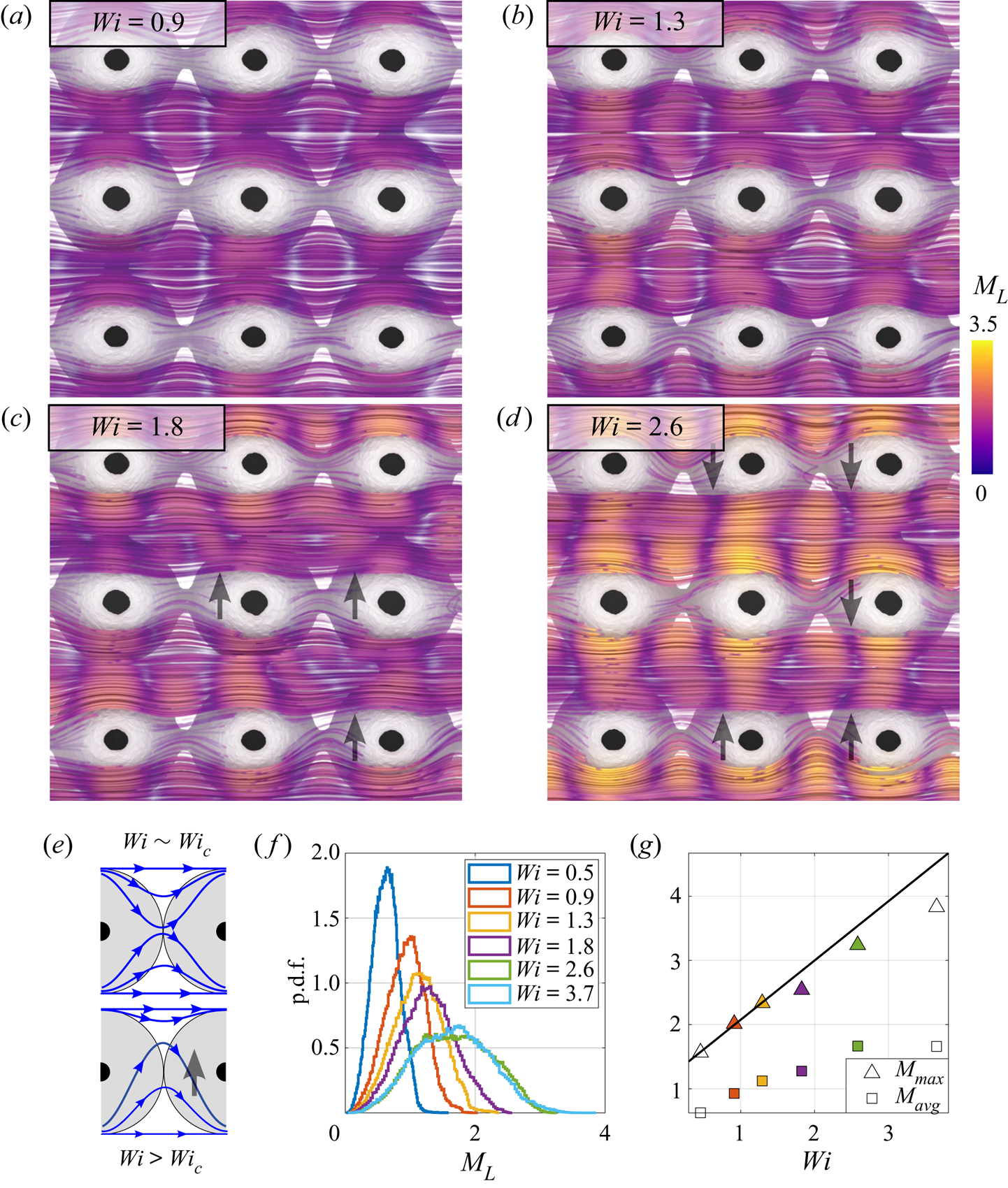
Figure 7. (a–d) Streamlines of local  $M_{L}$ evaluation for selected
  $Wi$ near
  $Wi_{c}$, with arrows highlighting asymmetry (sketch in (e)). ( f) The p.d.f. of the streamline fields. (g) The maximum and average
  $M_{L}$ at each
  $Wi$. Streamline curvature does increase with
  $Wi$ above
  $Wi_{c}$, but in doing so, symmetry is broken as streamlines flood towards neighbouring pores, thereby enforcing stability.
For  $Wi = 2.6$ (figure 7d), asymmetric flooding behaviour is shown more distinctly. Regions with this effect have been highlighted with arrows, and a sketch is shown in figure 7(e). Thus we infer that pores with elastically unstable flow will stabilize their peers as the instability manifests as a flooding incursion into neighbouring pores. Notably, this effect also correlates along the streamwise direction, such that rows of pores in
  $x^*$ show a similar flow response. Above
  $Wi_{c}$, we can see that local curvature and
  $M_{L}$ continue to increase with
  $Wi$, but at a reduced rate (figure 7g), owing to the overall distribution of
  $M_{L}$ tailing towards higher values but maintaining a similar mean (figure 7g). From
  $M_{max}$ in figure 7(g), we can estimate our critical
  $M_{c}$ for this geometry by taking
  $M_{max}$ at
  $Wi_c = 1.8$, yielding
  $M_{c} = 2.5$, with the caveat that although
  $M_{L}$ is self-consistent for different
  $Wi$, it will underestimate the theoretical
  $M$ due to discrete sampling limitations. Nonetheless,
  $M_{c}$ here is in good agreement with reported values of
  $M_{c}$ based on
  $M$ ranging from 1 to 7.
In the transient unstable state, spatial heterogeneity resolves the increased stresses via localized regions of increased flow instability. Although the pressure power spectra indicate that these pockets of instability must be transient, tomogram storage for masking remains computationally burdensome, thus instead we time-resolve the fluctuations of ET at high  $Wi$ where stronger low-frequency modes make it feasible to capture multiple state changes in the VOI within a 10 s recording. A sample description of the low-frequency velocity fluctuations is available for
  $Wi = 1.8$ in the Appendix. Moreover,
  $Wi_{c} \approx 2$ aligns with
  $De = \lambda U_{p}/ w_{p} = 1$ by definition, thus transient effects can grow in the array in this regime as polymer chains are advected between pores faster than they can relax.
3.3. Inter-pore heterogeneity
We consider the evolving flow state at  $Wi = 8.2$ as a representative case for ET. We support this assertion with selected power spectral densities extracted from a point in the velocity field (
 $x^* = z^* = 0$,
  $y^* = -0.75$) to expand upon the prior spectral analysis of the pressure field. In figure 8 we present the global
  $E_{pp}$ spectra discussed previously, together with local fluctuating crossflow velocity spectra
  $E_{vp}$, at
  $Wi = 3.7$ and
  $Wi = 8.2$. Here,
  $E_{vp}$ and
  $E_{pp}$ show the algebraic decays typical of ET: for
  $E_{pp}(f) \sim f^{-\beta }$ and
  $E_{vp}(f) \sim f^{-\alpha }$,
  $\beta \approx 3$ and
  $\alpha \approx 3.5$, consistent with a recent review (Steinberg Reference Steinberg2021). Furthermore, the analysis of Steinberg (Reference Steinberg2019) deduced a scaling relation
  $\beta = 2(\alpha -2)$ that supports our experimental data. The Taylor frozen flow hypothesis (Taylor Reference Taylor1938) has been applied reasonably well for parts of ET flow. Specifically, experiments and simulations have noted similarly steep decay exponents for the temporal and spatial power spectra (Burghelea et al. Reference Burghelea, Segre and Steinberg2005; Burghelea, Segre & Steinberg Reference Burghelea, Segre and Steinberg2007; van Buel & Stark Reference van Buel and Stark2022). Thus our scaling in the frequency domain will also track the wavenumber contribution in the spatial domain, yielding the common observation that ET is governed by the nonlinear interaction of only a few large-scale modes (Burghelea et al. Reference Burghelea, Segre and Steinberg2005; Steinberg Reference Steinberg2019).
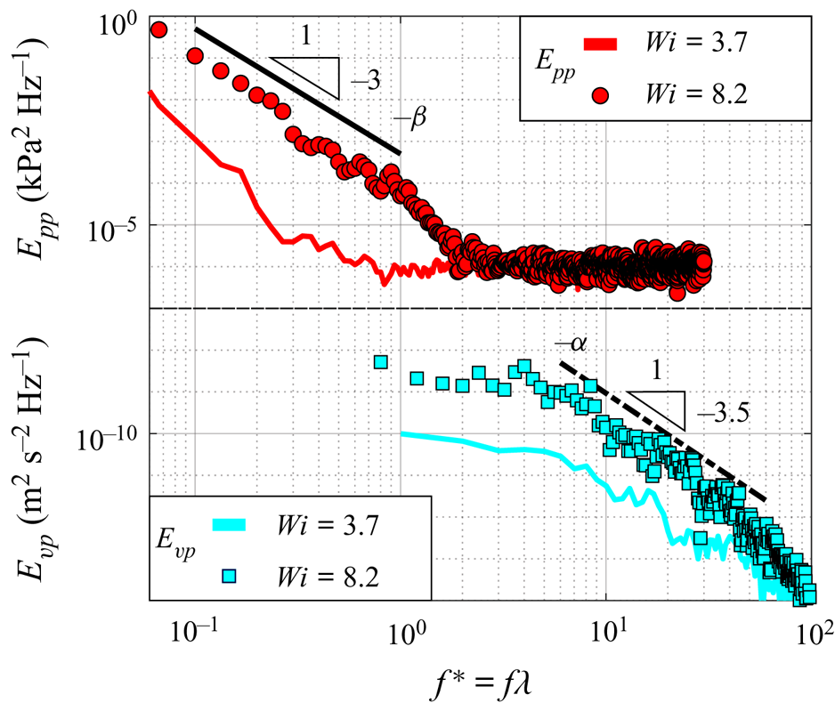
Figure 8. Power spectral densities of the fluctuation pressure  $E_{pp}(f)$ and the fluctuating crossflow velocity
  $E_{vp}(f)$ at moderate and high
  $Wi$. The power law decays for
  $E_{pp}(f) \sim f^{-\beta }$ and
  $E_{vp}(f) \sim f^{-\alpha }$ follow a scaling
  $\beta = 2(\alpha -2)$ (Steinberg Reference Steinberg2019).
For a local description of ET flow, in figures 9(a,b) we show streamlines coloured by  $\lvert \boldsymbol {u} \rvert ^*$ and
  $M_{L}$, respectively, to inspect local flow properties between the central rows of pores (labelled as
  $r_a$ and
  $r_b$, respectively). Generally, flow through row
  $r_a$ remains stable from pore columns 0–2, with a flow rate
  $\lvert \boldsymbol {u} \rvert ^*$ above the volume average, straightened streamlines, and low
  $M_{L}$. Flow through row
  $r_b$, however, has an opposite reaction for the same quantities: reduced
  $\lvert \boldsymbol {u} \rvert ^*$, strongly curving streamlines, and increased local
  $M_{L}$ across pore columns 1–3, but a reduction in pore 4. Remarkably, we can also see flow through
  $r_a$ transition to a state similar to flow through
  $r_b$ by pore 4, in this case driven by out-of-plane streamline curvature towards
  $+z^*$. Preceding the unstable flow in pore 4, we observe a reduction in
  $\lvert \boldsymbol {u} \rvert ^*$ in pore 3 as either the elastic instability or other rheological parameters drive increased pore resistance. Finally, we also see the same correlation behaviours noted in the prior section: streamwise correlation and crossflow inverse correlation of pores with unstable flow. The inversely correlated state is particularly compelling, with no
  $y^*$-adjacent pair of pores responding with mirrored unstable flow. This further supports our hypothesis that pore flooding can promote stability in adjacent pores. In pores farther from the unstable region, however, we do observe adjacent stable flow states, such as at
  $x^* = y^* = 0$ in figure 9. Therefore, the adjacent peer stabilization effect may be alternatively classed as a crossflow exclusion of instability. Streamwise correlation generally holds true, apart from the transition states noted in pores 3 and 4 as
  $r_a$ goes unstable and
  $r_b$ reduces curvature, respectively. A likely explanation for the streamwise consistency is flow history, which we will investigate by continuing this analysis throughout time in § 3.4.
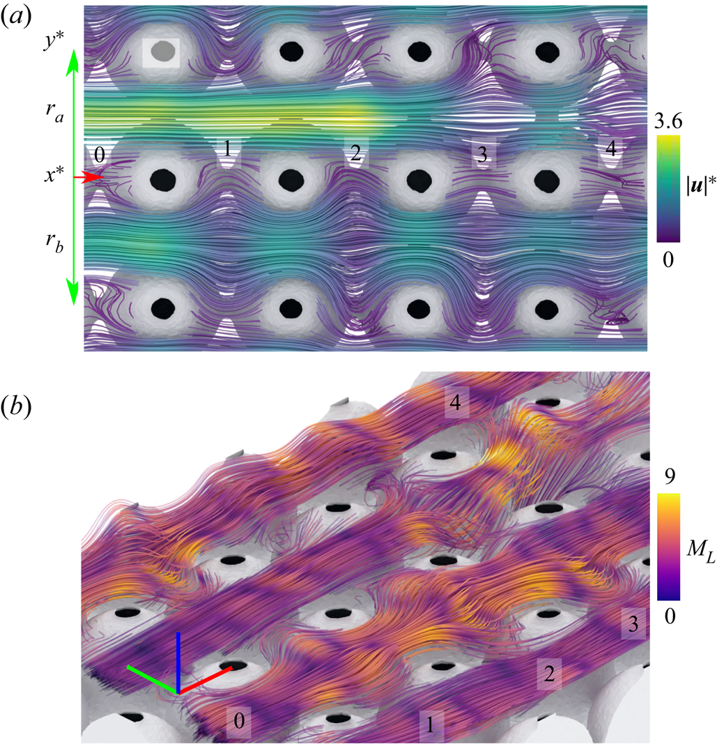
Figure 9. Instantaneous streamlines for the HPAA flow under a state of ET at  $Wi = 8.2$, coloured by (a) the dimensionless velocity magnitude
  $\lvert \boldsymbol {u} \rvert ^*$, and (b) the Pakdel–McKinley criterion
  $M_{L}$. We have numbered columns of pores along
  $x^*$.
To describe the laminar and unstable flow states, we take a snapshot also at  $Wi = 8.2$, but at an instant when
  $r_a$ and
  $r_b$ are in consistent states along
  $x^*$. Figure 10 presents both the local
  $M_{L}$ streamlines previously described together with planes of
  $\lvert \boldsymbol {u} \rvert ^*$,
  $v^*$,
  $\xi$ and
  $\dot {\gamma }$. Here,
  $r_a$ and
  $r_b$ have almost fully reversed their states from the figure 9 snapshot, with
  $r_a$ uniformly unstable between pores along
  $x^*$ and in
  $r_b$ repeating pores with laminar flow. Hence we can relate the instability to local rheological effects. As discussed previously, pores with unstable flow lead consistently to increased flow resistance (locally decelerated) compared to the laminar channel, but importantly, we see here that the laminar channel
  $r_b$ is also shear-dominated with strong rate-of-strain. The shear-thinning behaviour of the fluid is likely in effect, leading to a locally accelerated flow reaching
  $\lvert \boldsymbol {u} \rvert ^* = 3.6$. Along the unstable zone, we observe competing influences: while the fluid is strongly extensionally strain hardening, and these pores manifest with extensionally dominant flow, the rate-of-strain is locally reduced. Thus while strain hardening may be an influence in the evolution of the local instability, we cannot confirm this hypothesis in the present work.

Figure 10. (a,b) Instantaneous streamlines for the HPAA flow under a state of ET at  $Wi = 8.2$, together with (c–f)
  $x^*$–
 $y^*$ slices showing
  $\lvert \boldsymbol {u} \rvert ^*$,
  $\xi$,
  $v^*$ and
  $\dot {\gamma }$, respectively.
3.4. Feedback between streamline curvature and flow resistance
To describe the temporal evolution of the unstable flow state, we first refer back to the fluctuating pressure power spectra from figure 6(b). As we mentioned previously,  $f^* \approx 1$ appears to be a natural upper limit for the frequency of the spatiotemporal modes of ET as fluctuations approach
  $1/\lambda$ but decay rapidly at higher frequencies (figure 8). Therefore, we compare snapshots with a temporal stride of approximately
  $\lambda$, but with some variation permitted to capture disturbances evolving away from
  $\lambda$.
Selected streamline fields are presented in figure 11 to describe generally instability propagation forward in time. We start the sequence in figure 11(a), where an individual pore in the VOI is unstable (3, the last pore). All of the pores upstream of this point are stable in this row. Forward in time at  $t^* = 0.7$ (figure 11b), we see that pores 2 and 3 are now unstable; the unstable region has evidently propagated upstream. This trend continues for
  $t^* = 1.8$ and
  $2.8$ (figures 11c,d), with the full row now unstable at
  $t^* = 2.8$. Upstream propagation continues at
  $t^* = 3.9$ (figure 11e), with relaminarization occurring in pore 3. Clearly, flow history is important in this context, for both the onset of instability as well as the termination thereof. We support this notion by considering the streamline curvature of pores upstream of the local maximum
  $M_{L}$. The transition from a laminar state to a strongly unstable flow is spatially smooth, with streamline curvature and elastic stresses building for pores progressing along increasing
  $x^*$ towards a pore with a locally maximum state of instability (protruding streamlines). Positive feedback between streamline curvature and flow resistance is a likely explanation: in a given pore, local streamlines respond with increased curvature due to raised resistance in neighbouring pores downstream. In a given pore with unstable flow, streamlines protrude from the pore centre (figure 7e), and this excursion becomes more pronounced over time while being accompanied by locally increased flow resistance. Thereafter, flow in an adjacent pore upstream responds to the raised resistance with streamline protrusion, hence the instability propagates upstream in the array.
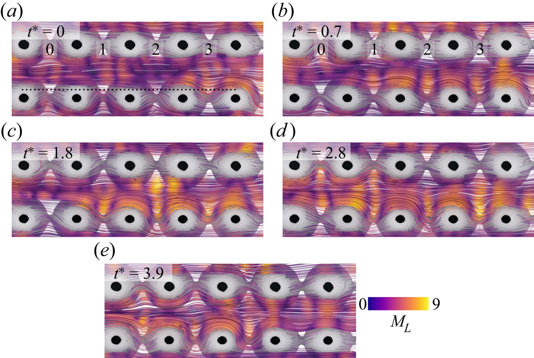
Figure 11. Snapshot streamline fields of  $M_{L}$ over selected
  $t^*$ at
  $Wi = 8.2$. Note that the black line in (a) indicates
  $y^* = -0.75$, which is used in figure 12.
To further explain the instability propagation, we present space–time diagrams in figure 12 extracted along  $y^* = \pm 0.75$ from separate recordings at the same
  $Wi = 8.2$. For reference, we also show the advection length scale
  $U_{p}\lambda /w_{p}$ overlaid on the figure. Here, we see that for a given point
  $x^*$, flow maintains a consistent laminar or unstable state over long
  $t^*$. Whereas for a time
  $t^*$, the fluctuating state persists over
  $x^*$ with a scale on a par with the advection length scale. Polymer chains in the flow would thus be in a state where strain is accumulated throughout a cohesive pocket of instability. Crossflow fluctuation may propagate rapidly upstream, as it does near
  $t^{*}_{0} = 2$ for
  $x^* = 2\unicode{x2013}3$, or the laminar state could linger as it does along
  $t^{*}_{0} = 2\unicode{x2013}4$ for
  $x^* = 1$. Similar behaviour is noted in the termination of instability shown in figure 12(b), where, for example, fluctuations decay along low
  $x^* = 0\unicode{x2013}2$ over a long time scale surpassing the recording limit. These time scales are not surprising when we compare the space–time diagrams to the fluctuating pressure power spectra from figure 6, where the lowest frequencies continued to gain power for decreasing
  $f^*$ towards the lower limit
  $0.06 f\lambda$ (period
  $17\lambda$). Thus although an upstream propagation speed of instability can be estimated roughly as
  $\approx$
 $-0.3U_p$, the progression from laminar to unstable flow is spatially smooth but not temporally, in support of the spectral characteristics of ET.
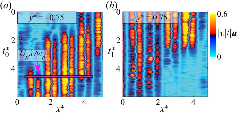
Figure 12. Space–time diagrams along  $y^* = \pm 0.75$ of the crossflow velocity magnitude ratio
  $|v|/|\boldsymbol {u}|$ from separate recordings at
  $Wi = 8.2$. We also include the advection length scale
  $U_{p}\lambda /w_{p}$ as the pink bar.
From our simplified ordered porous medium, we have elucidated viscoelastic flow effects relevant to porous media flow in particular, and to the evolution of vessel-scale modes for ET in general. Namely, we have highlighted the importance of spatial correlation via flow history effects as well as via communication between pore flow states. An area for further research, however, would be probing longer time scales; such are not feasible for a volumetric time-resolved study given current processing times, but a 2-D study of ET in our ordered porous medium would be a promising direction for future work, to better quantify the propagation nature of unstable flow near  $Wi_{c}$. Furthermore, while ET has been quantified in 3-D randomly packed media (Browne & Datta Reference Browne and Datta2021), packing structure and disorder are known to be significant for the onset of instability for viscoelastic flow (Walkama et al. Reference Walkama, Waisbord and Guasto2020; Haward et al. Reference Haward, Hopkins and Shen2021) and for chaotic mixing for creeping porous media flow (Turuban et al. Reference Turuban, Lester, Le Borgne and Méheust2018, Reference Turuban, Lester, Heyman, Le Borgne and Méheust2019), and these are thus topics of ongoing research.
4. Conclusions
From time-resolved measurements of dilute polymer flow through a refractive- index-matched novel arrayed porous medium, we have produced the first spatiotemporally complete description of elastic turbulence (ET). By reconstructing flow over multiple pores simultaneously, we can capture the local evolution of viscoelastic instability as flow evolves over a time span surpassing that of the polymer relaxation time  $\lambda$. Above a critical
  $Wi_{c} = 1.8$, a purely elastic instability occurs, leading to increased resistance, strongly curving streamlines and localized pore flooding, the last of which is an effect that actually stabilizes flow in neighbouring pores in crossflow by causing a reduction in streamline curvature there. The strongly fluctuating flow is accompanied by increased drag and in the spectral domain, steep power-law decays for velocity and pressure matching proposed ET scaling for
  $\alpha$ and
  $\beta$. In this state, we describe unsteady yet coexisting regions of laminar flow and unstable flow. We relate the spatially heterogeneous laminar zones to the local shear-thinning behaviour of the solution, but see low rate-of-strain with extensional flow in the resisting pores. We hypothesize that the pockets of instability are transient in nature and driven by locally raised downstream resistance acting as positive feedback on upstream streamline curvature. Whereas ET is typically characterized at the vessel scale, these new findings considering a flow volume developing over several vessel scales elucidate the significance of spatiotemporal correlation on the local evolution of ET.
Acknowledgements
We thank E. Chen, C. Browne and S. Datta from Princeton University for fruitful discussion. Under the Research Support Division at the Okinawa Institute of Science and Technology Graduate University (OIST), we also thank the Scientific Computing and Data Analysis section and the Engineering section for computation support and machining support, respectively.
Funding
We gratefully acknowledge the support of OIST with subsidy funding from the Cabinet Office, Government of Japan. We also acknowledge financial support from the Japanese Society for the Promotion of Science (JSPS, grant nos 21K14080 and 21K03884).
Declaration of interests
The authors report no conflict of interest.
Data availability statement
Raw data are available upon reasonable request from the authors.
Author contributions
Conceptualization by D.W.C., A.Q.S. and S.J.H.; methodology by D.W.C., K.T-P. and S.J.H.; fabrication by K.T-P.; writing by D.W.C., A.Q.S. and S.J.H.; supervision by A.Q.S.; funding acquisition by D.W.C., S.J.H. and A.Q.S. All authors have read and agreed to the published version of the manuscript.
Appendix
We describe a weakly transient flow state near the critical  $Wi_{c}$. From the trend of the power spectra, we expect this state to gain power across progressively higher frequency modes as
  $Wi$ is increased. To validate that
  $Wi = 1.8$ is indeed transient, we present sample streamlines coloured by
  $M_{L}$ for two arbitrary snapshots, along with the change in crossflow velocity
  ${\rm \Delta} v / U_p$ from a slice of the background grid, in figure 13. Clearly, the flow is weakly transient, so we quantify the temporal evolution of ET at higher
  $Wi$ as a generalized description of the unstable state.
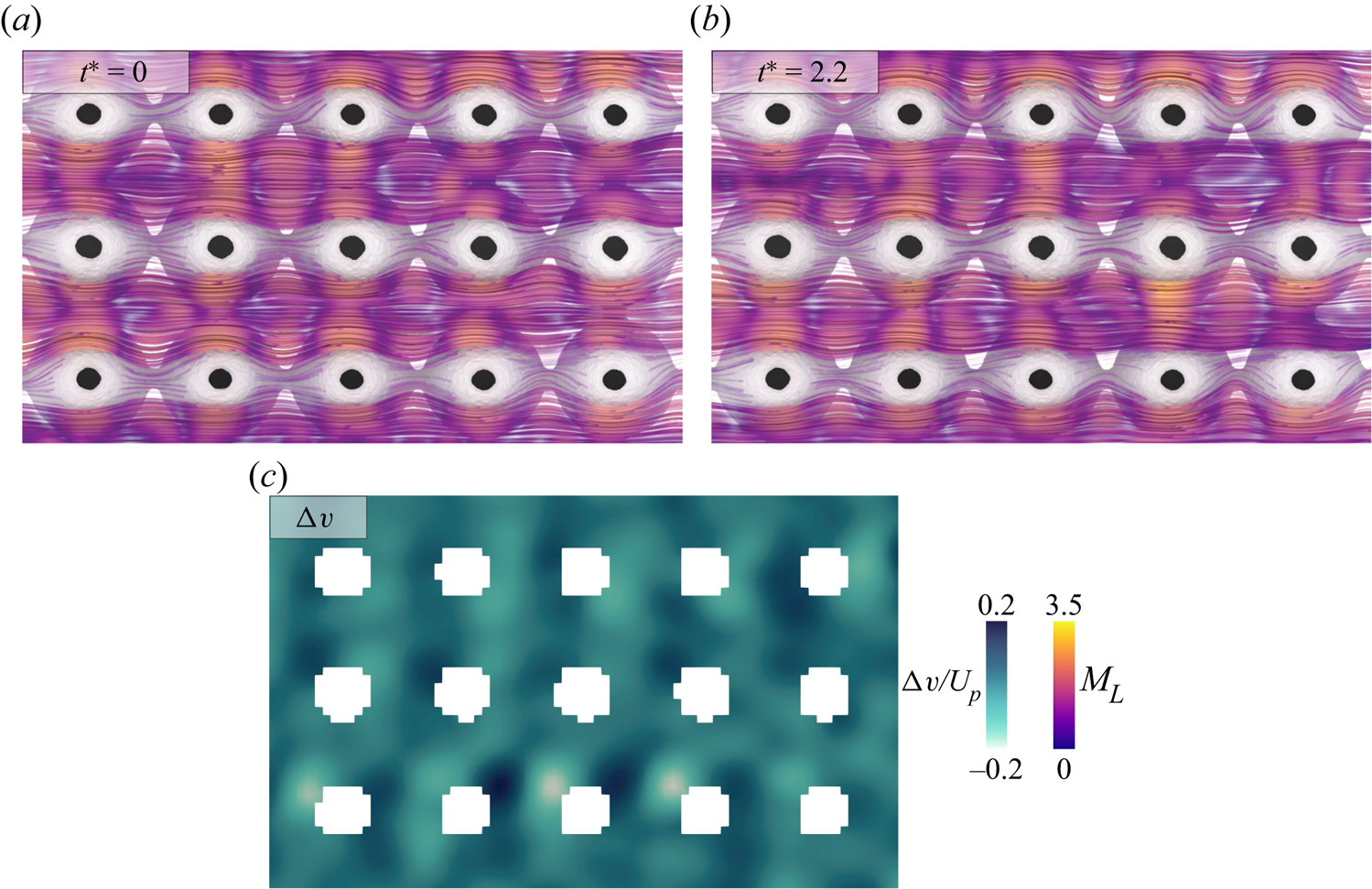
Figure 13. (a,b) Streamlines coloured by  $M_{L}$ at
  $Wi = 1.8$; after the onset of instability, the flow is weakly transient with (c) minor velocity fluctuations.


 Open access