


Introduction
Animal and plant breeders are often concerned with the improvement of complex traits. A new approach called ‘genome-wide selection’ or ‘genomic selection’ (GS) (Meuwissen et al., Reference Meuwissen, Hayes and Goddard2001), based on genome-wide marker profiling, can accelerate the genetic improvement of such traits. GS means using genomic information to evaluate and select potential candidates. A key feature of this method is that the entire genome is covered by dense markers. When several thousand markers are genotyped throughout the genome, it is assumed that the markers are next to the causal mutations and, therefore, capture and reflect causal effects. All genetic variance is justified by these markers and it is assumed that the markers are in linkage disequilibrium (LD) with quantitative trait loci (QTL) (Goddard and Hayes, Reference Goddard and Hayes2007; de Roos et al., Reference de Roos, Hayes, Spelman and Goddard2008). Single nucleotide polymorphism markers (SNPs) are the most abundant type of DNA polymorphism in the genome, have lower mutation rates and are easily genotyped, and that is why they are used for GS. The individual effect of each SNP is calculated using both genotypic and phenotypic data with statistical methods and by summing up the effects of all SNPs, the genomic estimated breeding values (GEBVs) of individuals are estimated. Thus, QTL analysis for working out marker–trait associations is not needed (Kumar et al., Reference Kumar, Pratap, Solanki, Gupta, Goyal, Chaturvedi, Nadarajan and Kumar2012). Although GS was introduced in 2001, its application delayed until availability of high-density SNP panels for genotyping of animals (Van Tassell et al., Reference Van Tassell, Smith and Matukumalli2008). GS has contributed significantly to increase genetic gain for a variety of economically important traits, both in animal (Van Raden Reference Van Raden2008; Szyda et al., Reference Szyda, Żukowski, Kamiński and Żarnecki2013) and plant species (Kumar et al., Reference Kumar, Pratap, Solanki, Gupta, Goyal, Chaturvedi, Nadarajan and Kumar2012; Brito et al., Reference Brito, Oliveira and Oliveira2017). In GS, increase in genetic gain arises from shorter generation interval, increased intensity of selection and greater precision in the selection of animals for breeding (Klímová et al., Reference Klímová, Kašná, Machová, Brzáková, Přibyl and Vostrý2020).
Many traits of biological and economic importance follow a discontinuous distribution, but their inheritance is not simply Mendelian such as susceptibility to disease with two phenotypic categories of affected and non-affected, degree of dystocia and the number of progenies in a delivery. These traits are termed ‘threshold traits’. They are quantitative traits that are discretely expressed in a limited number of phenotypes (usually two), but which are based on an assumed continuous distribution of factors that contribute to the trait (latent variable, liability) (Falconer and Mackay, Reference Falconer and Mackay1996; Roff et al., Reference Roff, Stirling and Fairbairn1997). At first, these traits were seemed a bit out of the quantitative genetic theory, but when exposed to genetic analysis, it was revealed that their inheritance was similar to that of quantitative traits. These traits have inherently continuous changes, but due to having threshold, apparently they have discontinuous changes (Falconer and Mackay, Reference Falconer and Mackay1996). Literally, threshold is a level, point or value above which something is true or will take place and below which it is not or will not (Fig. 1). This idea of applying a threshold to a Gaussian hypothetical trait can be traced back to even earlier work by Pearson (Reference Pearson1900). When the latent variable (e.g. a biochemical material in the blood with normal distribution in the population) is below this threshold, the individuals show normal phenotype, and when the latent variable overrides the threshold, another phenotypic class is revealed (affected). Therefore, while latent variable has normal distribution, the observed variable follows a discrete distribution with a few phenotypic classes (de Villemereuil, Reference de Villemereuil2018). The basis of threshold characters is a combination of several physiological and developmental processes (Gianola, Reference Gianola1982). Changes in these traits have both genetic and environmental origins and can be measured and studied as a quantitative trait in the routine way. González-Recio and Forni (Reference González-Recio and Forni2011) performed a genomic evaluation for scrotal hernia in pig with one threshold and reported that the accuracy of genomic evaluation was very low. The effect of the number of threshold on the accuracy of genomic evaluation has not been studied so far. Therefore, this study was conducted to study the effect of threshold number on the accuracy of genomic evaluation of discrete traits. In addition, the predictive performance of genomic best linear unbiased prediction (GBLUP) (Van Raden, Reference Van Raden2008), support vector machine (SVM) (Boser et al., Reference Boser, Guyon and Vapnik1992) and Bayesian method B (BayesB) (Meuwissen et al., Reference Meuwissen, Hayes and Goddard2001) in genomic evaluation of discrete traits was also studied.
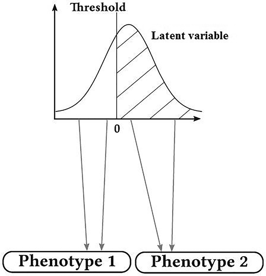
Fig. 1. Graphic representation of a trait with one threshold (de Villemereuil, Reference de Villemereuil2018).
Materials and methods
Population and genome
Population and genome were simulated using hypred package (Technow, Reference Technow2013) in R software (R Development Core Team, 2021). The focus of the package is on producing data for genomic applications in applied genetics, namely genomic prediction and selection. In a script, we listed the instructions that hypred should use for simulation of genome. Parameters such as number of chromosomes, length of each chromosome, number of SNPs and QTLs per chromosome and distribution of QTL effects were listed in the script. Hypred executed the instructions in the script and built the genome with several internal functions such as hypredGenome (used to define the genome parameters), hyprednewQTL (used to assign QTLs), hypredRecombine (used to simulate meiosis), hypredNewMap (used to modify the genetic map), etc.
A genome consisting of three chromosomes, each one Morgan length, was simulated and 3000 SNPs were uniformly distributed on it. Coding for each genotype with alleles A1 and A2 were, respectively, 2 for A1A1, 0 for A2A2 and 1 for A1A2 or A2A1. The mutation rate at the marker loci was 2.5 × 10⁻³ to provide a high probability of polymorphic marker loci. This was 2.5 × 10⁻⁵ per locus per generation for each QTL (Meuwissen et al., Reference Meuwissen, Hayes and Goddard2001). Gamma distribution of QTL effects was considered, with shape (β) and scale parameters as 0.4 and 1.66, respectively (Meuwissen et al., Reference Meuwissen, Hayes and Goddard2001).
The baseline population was simulated to be 100 individuals (50 males and 50 females) and randomly mated for 50 generations to create LD between the markers and QTLs. Because two progenies were born from both parents during 50 generations of random mating, the population size was constant throughout the generations of the historical population. In other words, the effective population size (Ne) was 100. The chromosomal compositions of the offspring were obtained by random sampling of the paternal and maternal chromosomes. In generation 51, the population was expanded to 1000 individuals and considered as the reference population. These individuals had both genotypic and phenotypic information. Thereafter, random mating was used for another generation. The animals in the generation 52 had known genotypes but without phenotypic records, which treated as validation population for which genomic breeding values had to be predicted. Thus the genotypic matrix included the genotypic information of 1000 individuals which were genotyped for 3000 SNPs. Parameters used for the simulation of genome are listed in Table 1. In order to convert the normal phenotype into a threshold, the Probit function (Gianola, Reference Gianola1982) was used. Using Probit function the phenotypic category of each individual is determined according to the individual's phenotypic value and the threshold points.
Table 1. Parameters used for simulation program

Scenarios under study
The main purpose of this study was to investigate the threshold number on the accuracy of genomic evaluation. Therefore, by applying 1, 2, 3, 4, 5 and 6 thresholds, traits with 2, 3, 4, 5, 6 and 7 phenotypic classes were simulated, respectively. The number of QTLs was defined as a ratio to the number of markers so that in two different scenarios, 1 and 10% of the number of markers were considered as QTL (30 and 300 QTLs, respectively). In addition, three levels of heritability (0.10, 0.30 and 0.50) were also considered for simulation of phenotypes.
Methods of genomic evaluation
Genomic best linear unbiased prediction (GBLUP)
The GBLUP was fitted as follows:

where y is the vector of phenotypic observations, Z is the design matrix associating phenotypic observations to GEBVs, g is the vector of genomic breeding values and assumed that g~N(0,G$\delta _g^2$ ) where $\delta _g^2$
 is the additive genetic variance, and G is the genomic relationship matrix whose elements estimated based on allelic similarity between individuals (Van Raden, Reference Van Raden2008). The GBLUP was run using package BGLR in R (de los Campos and Perez Rodriguez, Reference de los Campos and Perez Rodriguez2018).
Support vector machines (SVM)
One of the kernel methods is the SVM. Kernel methods can be thought of as instance-based learners. Rather than learning some fixed set of parameters corresponding to the features of their inputs, they ‘remember’ the i-th training example. In case of GS the input is genotypic and phenotypic information of animals in the reference population (xi, y i) and SVM learns for it a corresponding weight w i. Prediction of unlabelled inputs, i.e. those not in the training set (i.e. phenotypic information of candidate animals ($\hat{y}$ )) is treated by the application of a kernel between the unlabelled input x′ and each of the training inputs, xi. For quantitative responses, support vector regression (SVR) is used. The SVR uses linear models to implement non-linear regression by mapping the input space (the marker data set) to a feature space of a different dimension (lower in the case of GS) using a non-linear kernel function followed by linear regression in this feature space. In SVR, with input data set $G = \{ ( {\boldsymbol x}_{\boldsymbol i}, \;d_i) \} _i^n$
 (where xi is the input vector, di is the desired real-valued labelling and n is the number of the input records), x is first mapped into a higher-dimension feature space F via a non-linear mapping Θ, then linear regression is performed in this space. In other words, SVR approximates a function using the following equation (Liu et al., Reference Liu, Meng, Xu, Flower and Li2006; Hastie et al., Reference Hastie, Tibshirani and Friedman2009):

The coefficients w and b are estimated by minimizing:

where Lɛ (d, y) is the empirical error measured by ɛ-insensitive loss function

and the term 1/2||w||2 is a regularization term. The constant C is specified by the user, and it determines the trade-off between the empirical risk and the regularization term. The ɛ is also specified by the user, and it is equivalent to the approximation accuracy of the training data. The estimates of w and b are obtained by transforming Eqn (*) into the primal function:

By introducing Lagrange multipliers, the optimization problem can be transformed into a quadratic programming problem. The solution takes the following form:

where K is the kernel function K(x, xi) = Θ(x)T Θ(xi). By using a kernel function, we can deal with the problems of arbitrary dimensionality without having to compute the mapping Θ explicitly. Different kernel functions can be selected to map (or transform) input data to feature space. According to Kasnavi et al. (Reference Kasnavi, Aminafshar, Shariati and Emam Jomeh Kashan2018), we used radial kernel to construct SVM. The package e1071 (Meyer et al., Reference Meyer, Dimitriadou, Hornik, Weingessel and Leisch2013) was used for SVM analysis.
Bayesian method B (BayesB)
In this model, it is assumed that only part of the loci explains the entire genetic variance, and many loci do not play a role in genetic variance. BayesB can be written as follows:

where y is the phenotype of the animal i, μ is the mean, k is the number of marker loci, x is the genotype of the marker at the locus j (i th allele) which is encoded as 0, 1 and 2 (number of copies of the SNP allele carried by the i th animal). βj is the effect of allelic substitution at position j and δj which is coded as 0 and 1 indicates the absence (with probability π) or the presence (with probability 1–π) of the locus j in the model.


The main assumption of this method is that many SNPs are located in genomic regions that have no specific QTL association and have no effect on the trait and only a small part of SNPs are in LD with QTLs and therefore have an effect. In general, π represents the expected ratio of SNPs which are in LD with QTLs to the total SNP number. The effects of SNPs will be sampled from the t-distribution, but the variance of the effects will be sampled with probability π from a scaled inverse χ 2 distribution (Meuwissen et al., Reference Meuwissen, Hayes and Goddard2001):


To implement BayesB, BGLR package (de los Campos and Perez Rodriguez, Reference de los Campos and Perez Rodriguez2018) was used. Gibbs sampling algorithm was used to sample conditional posterior distribution of marker effects. Marker effects were inferred using 12 000 sample chains (2000 burning samples and the next 10 000 samples for posterior distribution inferences).
Accuracy of GEBV
The Pearson's correlation between the predicted genomic breeding values and the true genomic breeding values (rp,t) was used as an indicator of the accuracy of genomic evaluation. Each scenario which was a combination of heritability level, QTL number and method used was analysed 100 times and the average accuracy of each scenario was presented.
Results
The effect of threshold number on the accuracy of genomic evaluation in different scenarios of QTL number and heritability level is shown in Fig. 2. As observed, by increasing the number of threshold from 1 to 6 thresholds, the accuracy of genomic evaluation increased. For SVM, by increasing the number of threshold from 1 to 6 thresholds, in different scenarios of heritability level (0.1, 0.3 and 0.5), the accuracy of prediction increased by 49, 29 and 24%, respectively. For GBLUP, in similar scenarios of heritability level, by increasing the number of thresholds from 1 to 6 thresholds, the accuracy of prediction increased by 27, 21 and 27%, respectively. Also, 22, 21 and 19% increase in accuracy was observed for BayesB following increase in the number of threshold from 1 to 6 thresholds. The increase in prediction accuracy was more noticeable when the number of threshold increased from 1 to 2 thresholds compared with scenarios in which the number of threshold increased from 2 to 3 and beyond. For example, for SVM and at the heritability level of 0.1, by increasing the number of threshold from 1 to 2 thresholds, the prediction accuracy increased by 47%, while by increasing the number of threshold from 2 to 3 thresholds, the prediction accuracy increased by only 6%.

Fig. 2. The effect of threshold number on the accuracy of genomic evaluation.
The average prediction accuracy of the SVM, GBLUP and BayesB in different scenarios of heritability level and QTL number is shown in Fig. 3. On average, in the scenario of heritability = 0.1, the SVM showed a very poor performance, so that its prediction accuracy was significantly lower than the GBLUP and BayesB (P < 0.05). By increasing heritability to 0.3 and then to 0.5, the prediction accuracy of all three methods increased; however, even at higher levels of heritability, GBLUP and BayesB kept their distance with SVM. With one threshold, BayesB performed better than the SVM and GBLUP, though its difference with the GBLUP was not significant in most cases (P > 0.05) (Figs 2(a)–(c)). In general, in most studied scenarios, the BayesB and GBLUP had better performance than SVM.

Fig. 3. Comparison of methods in different scenarios of heritability level and QTL number (the accuracy of each method is the average of the results of the 1, 2, 3, 4, 5 and 6 thresholds scenarios).
The effect of heritability on the prediction accuracy is shown in Fig. 4. In all methods, the accuracy of genomic evaluation increased with increasing heritability. When the trait had one threshold and was controlled with 30 QTLs, by increasing heritability from 0.1 to 0.5, the prediction accuracy for SVM, GBLUP and BayesB increased by 62, 41 and 45%, respectively. It was 52, 44 and 49% when trait was controlled by 300 QTLs.

Fig. 4. The effect of heritability on the accuracy of genomic evaluation.
In most of the scenarios, following change in the number of QTLs from 30 to 300 QTLs, no significant change in the accuracy of genomic evaluation was observed. In some cases, with increasing QTL number, the accuracy of prediction decreased slightly, and in other cases, a slight increase was observed (Fig. 5).

Fig. 5. The effect of QTL number on the accuracy of genomic evaluation.
Discussion
So far, most studies in the field of GS have been conducted on continuous traits and little efforts have been made for genomic evaluation of threshold traits, though many traits that significantly affect profitability belong to the threshold traits category. Gianola (Reference Gianola1982) and Gianola and Foulley (Reference Gianola and Foulley1983) founded the mathematical theory for genetic analysis of threshold traits. Due to the fact that threshold traits occur discretely, the use of linear models cannot bring much genetic improvement for these traits. Deljoo-Issa-Lou (Reference Deljoo-Issa-Lou2013) reported that evaluation of threshold traits using pedigree-based threshold models cannot be highly reliable and suggested using genomic information to improve these traits. There are no previous reports on the effects of threshold number on the accuracy of genomic evaluation which makes comparison difficult. González-Recio and Forni (Reference González-Recio and Forni2011) simulated a discrete trait with a threshold and predicted genomic breeding values using different parametric and non-parametric methods. The accuracy of genomic evaluation for all methods was low with a maximum value of 0.41, which is in consistent with the results of the present study. However, they did not evaluate traits with threshold number higher than one. As a result, for traits with one threshold such as durability and liability to disease, the accuracy of genomic evaluation would be low. Therefore, methods with maximum prediction accuracy should be used for genomic evaluation of such traits. For traits with more than one threshold such as littler size in sheep, degree of calving difficulty, conformation and type scores, fortunately we can achieve accuracy similar to continuous traits by applying traditional genomic evaluation methods.
A result we noticed was that in some cases (mostly at heritability = 0.1, Fig. 2(a)), by increasing threshold number, the accuracy decreased (e.g. comparing accuracy of BayesB in 5 and 6 thresholds scenarios, the accuracy was higher in the 5 thresholds scenario). At low levels of heritability, greater environmental noises affect the power of models to extract small additive genetic effects leading to fluctuation in the estimates of genomic breeding values (Kasnavi et al., Reference Kasnavi, Aminafshar, Shariati and Emam Jomeh Kashan2018). It can result in random changes in the accuracy of GEBVs. In such a situation, higher accuracy at lower number of threshold would be expected.
Most studies have focused on Bayesian models to analyse threshold traits. Wang et al. (Reference Wang, Woodward, Bauck and Rekaya2012) by analysing threshold traits by Bayesian models reported that the accuracy of the BayesB and BayesC was almost similar and was higher than BayesA. Villanueva et al. (Reference Villanueva, García-Cortés, Toro, Varona and Daetwyler2011) reported that genomic evaluation of threshold traits with BayesB significantly increases the accuracy of genomic breeding values compared to linear models. The rate of increase in the accuracy of genomic breeding values obtained by Bayesian model compared to linear models for threshold traits ranged from 4% (at heritability 0.3) to 16% (at heritability 0.1). Baneh et al. (Reference Baneh, Nejati Javaremi, Rahimi-Mianji and Honarvar2017) also compared Bayesian methods including Ridge regression, BayesA, BayesB, BayesC and BayesL in genomic evaluation of threshold traits. Their results showed that the accuracy of prediction of all studied methods (due to similarity of computational nature) was close to each other, but in the meantime, BayesA and BaysB were able to estimate SNP effects slightly better (3–7%) than other methods. A Bayesian association mapping for threshold traits using a threshold model was also proposed by Iwata et al. (Reference Iwata, Ebana, Fukuoka, Jannink and Hayashi2009) and their approach could reduce both false-positive and false-negative rates in detecting QTL to reasonable levels.
Recent studies have shown the significant effect of heritability on the accuracy of genomic evaluation. For example, Hayes et al. (Reference Hayes, Daetwyler, Bowman, Moser, Tier, Crump, Khatkar, Raadsma and Goddard2010) examined the effect of different levels of heritability on the accuracy of genomic evaluation and reported that at heritability levels of 0.1, 0.3, 0.5, 0.7 and 0.9, the accuracy of genomic evaluation was 0.35, 0.5, 0.60, 0.65 and 0.72, respectively. Mohammadi Chamachar et al. (Reference Mohammadi Chamachar, Hafezian, Honarvar and Farhadi2015) reported that accuracy of genomic evaluation of a trait with heritability of 0.05, 0.1 and 0.25 was 0.79, 0.82 and 0.87, respectively. Naderi (Reference Naderi2018) reported that for production traits with heritability of 0.3, higher prediction accuracy (0.67) was obtained than a trait with 0.05 heritability (0.41). Zhang et al. (Reference Zhang, Wang, Beyene and Semagn2017) by studying the effect of marker density, reference population size and trait heritability reported that among the studied factors, heritability had the greatest impact on the accuracy of genomic evaluation. High heritability shows a higher ratio of genetic variance to phenotypic variance and means a smaller role of environmental noises in the phenotypic variation of the trait. Therefore, the additive genetic effect which is captured by each marker increases. In such a situation, the power of model to extract such greater individual additive effects increases leading to increased accuracy (Ahmadi et al., Reference Ahmadi, Ghafouri-Kesbi and Zamani2021; Ashoori-Banaei et al., Reference Ashoori-Banaei, Ghafouri-Kesbi and Ahmadi2021). Goddard (Reference Goddard2009) showed that in order to achieve a certain degree of accuracy, traits with lower heritability require more phenotypic records in the reference group, but this trend was not linear. In other words, the effect of doubling the number of phenotypic records for low heritability traits is greater than the effect of doubling the number of phenotypic records for high heritability traits.
Foroutanifar (Reference Foroutanifar2017) reported that the prediction accuracy of BayesA, BayesB and BayesC methods was higher than BayesL and BayesR in the scenarios of small number of QTLs, but with increasing the number of QTLs to 150 and more, this advantage was completely disappeared. Coster et al. (Reference Coster, Bastiaansen, Calus, van Arendonk and Bovenhuis2010) showed that when Bayesian regression and Bayesian LASSO fitted to the data, with decreasing QTL number, higher accuracy was obtained but the accuracy of least squares method (Partial Least Squares [PLS]) was not affected by QTL number. Comparing different Bayesian methods for genomic evaluation of threshold traits, Wang et al. (Reference Wang, Woodward, Bauck and Rekaya2012) observed that Bayesian methods B and C were sensitive to the number of QTLs, and the accuracy of estimates decreased with increasing the number of QTLs from 20 to 500. Also, by comparing Bayesian methods B and GBLUP, Daetwyler et al. (Reference Daetwyler, Hickey and Henshal2010) observed that the accuracy of GBLUP was constant in different scenarios of number of QTLs, but the accuracy of BayesB was higher in scenarios of small number of QTLs. Assuming a constant total genetic variance, by increasing the number of QTLs, total genetic variance is distributed to a large number of QTLs. In other words, the contribution of each QTL in the total genetic variance decreases and in such a situation, the efficiency of models for estimating such small effects decreases. In addition, as the number of QTLs increases, more markers are needed to capture the effects of all QTLs (Habier et al., Reference Habier, Fernando and Dekkers2009). Therefore, increase in the number of QTLs can lead to increase in the accuracy of genomic evaluation if the number of markers increases as well.
In conclusion, genomic evaluation of traits with one threshold had low accuracy and with increasing the number of thresholds, the accuracy of genomic prediction increased. The SVM showed a poor performance in predicting genomic breeding values, especially when the studied trait had only one threshold. GBLUP and specially BayesB showed better performance in genomic evaluation of threshold traits compared to SVM. While increase in the level of heritability increased the prediction accuracy, change in the QTL number had little effect on the accuracy of genomic evaluation.
Author contributions
M. Ghasemi performed the formal analyses. F. Ghafouri-Kesbi designed the study and wrote the original draft. P. Zamani contributed to formal analyses.
Financial support
This research received no specific grant from any funding agency, commercial or not-for-profit sectors.
Conflict of interest
The authors declare no conflicts of interest between authors and other people, institutions or organizations.
Ethical standards
Not applicable.


