


1. INTRODUCTION
Relative position awareness is a key factor for many applications such as Intelligent Transportation Systems (ITS) and Location-Based Services (LBS) (Tatchikou et al., Reference Tatchikou, Biswas and Dion2005). One way to obtain position, Global Navigation Satellite Systems (GNSS), is widely used in ITS. Unfortunately, current commercially available GNSS receivers suffer positioning error up to tens of metres, which cannot satisfy some safety-critical applications, such as collision avoidance and lane-level guidance. Recently, advances in wireless networks have encouraged the development of Cooperative Positioning (CP) in Vehicular Ad Hoc Networks (VANETs) (Wymeersch et al., Reference Wymeersch, Lien and Win2009; Boukerche et al., Reference Boukerche, Oliveira, Nakamura and Loureiro2008; Patwari et al., Reference Patwari, Ash, Kyperountas, Hero, Moses and Correal2005). Through communicating measurements among the vehicles, CP can improve the performance of absolute and relative positioning.
So far, several CP techniques have been considered for improving the positioning in VANETs. Some typical CP techniques are Differential Global Positioning System (DGPS) (Kaplan and Hegarty, Reference Kaplan and Hegarty2006), Real-Time Kinematic (RTK) (Hofmann-Wellenhof et al., Reference Hofmann-Wellenhof, Lichtenegger and Collins2001), and satellite/ground-based augmentation systems (Christie et al., Reference Christie, Ko, Hansen, Dai, Pullen, Pervan and Parkinson1999). However, these techniques rely on infrastructure and cannot perform well in urban environments due to limited view of the sky, multipath and non-line-of-sight issues from nearby buildings.
Recently, some range-based CP techniques in wireless networks (Parker and Valaee, Reference Parker and Valaee2007; Patwari et al., Reference Patwari, Hero, Perkins, Correal and O'Dea2003) have been proposed to overcome these problems, which achieve positioning through fusing the range and GNSS measurements (Venkatraman et al., Reference Venkatraman, Caffery and You2002; Alam et al., Reference Alam, Balaie and Dempster2010; Richter et al., Reference Richter, Obst, Schubert and Wanielik2009). The range-based CP techniques rely on radio-based methods, such as Time Of Arrival (TOA), Time Difference Of Arrival (TDOA), Angle Of Arrival (AOA), and Received Signal Strength (RSS), which normally require sensors with high computational complexity and/or suffer from inadequate ranging accuracy. Meanwhile, radio ranging was identified as impractical by Alam et al. (Reference Alam, Balaie and Dempster2009). To avoid the challenges and complexities of range-based CP methods, another class of CP techniques, based on range-rating, was proposed by Arias et al. (Reference Arias, Lazaro, Zuloaga. and Jimenez2004), Xu et al. (Reference Xu, Shen and Yan2009) and Alam et al. (Reference Alam, Balaie and Dempster2011). Based on the Doppler effect, Arias et al. (Reference Arias, Lazaro, Zuloaga. and Jimenez2004) presented a localisation algorithm to estimate the position of a moving target in a wireless sensor network. However, the optimal geometry of the vehicular network for this method is not consistent with the geometry of the vehicular environment in urban streets. Xu et al. (Reference Xu, Shen and Yan2009) proposed a Doppler shift-based CP method for VANETs, but the method relies on fixed infrastructure as anchor nodes. By utilising the Doppler shift of the carrier of a Dedicated Short-Range Communications (DSRC) link between two vehicles, a loose integration CP approach was proposed by Alam et al. (Reference Alam, Balaie and Dempster2011), which showed a performance improvement of up to 48% against standalone GPS. However, this method cannot eliminate spatially correlated errors among vehicles, such as satellite clock error, ionosphere error, and troposphere error. Moreover, the loose integration CP approach is based on GPS position data. Therefore, it cannot work in partial GPS outage environments where fewer than four GPS satellites are still observable. By adopting double differencing principles, a tight integration CP technique was proposed by Alam et al. (Reference Alam, Balaie and Dempster2013a), which fuses low-level GPS data, i.e. pseudoranges, among the participating vehicles. This method eliminates spatially correlated errors among vehicles and achieves higher performance in relative positioning compared to DGPS. Furthermore, based on this method, an INS-aided enhanced tight integration CP approach for relative positioning was proposed (Alam et al., Reference Alam, Kealy and Dempster2013b), which showed a performance improvement over a purely tight integration CP. But the Doppler shift based on DSRC was not introduced in this tightly-coupled approach. Meanwhile, this method relies on GPS Doppler measurements to obtain the rotation angles of the body frame to navigation frame, therefore an increased duration of GPS outage results in performance degradation with respect to the INS-integrated method shown in this paper. Therefore the methods proposed by (Alam et al., Reference Alam, Kealy and Dempster2013b) are not suitable for dense urban areas where observable GPS Doppler measurements are low.
In this paper, we propose a novel tight integration CP method based on low-cost IMU and DSRC Doppler shift for application in dense urban areas. In this method, the GPS pseudoranges and GPS Doppler shifts, along with the IMU measurements, are shared among the participating vehicles, and the DSRC Doppler is estimated through the Carrier Frequency Offset (CFO) (Tao et al., Reference Tao, Wu and Xiao2009; Alam, Reference Alam2011). Then each vehicle fuses the GPS measurements, IMU data and DSRC Doppler to obtain its relative position. In comparison to Alam et al. (Reference Alam, Kealy and Dempster2013b), the rotation angles of the body frame to navigation frame in this paper are calculated from the Kalman filter states, which are effectively smoothed. This implementation results in a significantly slower deterioration of positioning errors in low GPS visibility environments. The performance of the proposed method is verified by analytical and experimental results. Experimental results show that, in the full GPS coverage environment, our proposed method improves upon existing methods, namely the tight CP with INS (Alam et al., Reference Alam, Kealy and Dempster2013b), tight CP (Alam et al., Reference Alam, Balaie and Dempster2013a) and DGPS (Kaplan and Hegarty, Reference Kaplan and Hegarty2006), in terms of precision, at least by 6%, 15%, and 28%, respectively, and in a complete GPS outage environment, the performance improvement in Root Mean Square Error (rmse) achieved is up to 60%, 55%, and 66%, respectively, when the GPS outage duration is 20 seconds.
2. PROBLEM DEFINITION AND SOLUTION DESIGN
Assume a VANET is combined with a number of vehicles in a dense urban area, and it is also assumed that all the vehicles are equipped with a GPS receiver, a Micro-electromechanical System (MEMS) -based IMU and a DSRC transceiver to communicate their data. The ultimate goal is that each vehicle can estimate its relative position to its neighbours using a data fusion algorithm which is fed by GPS and IMU observations with the DSRC Doppler and those of the neighbours received through vehicle-vehicle communication by DSRC.
2.1. The GPS observations
Several sources contribute to the errors in pseudorange measurements. Specifically, the pseudorange observable between receiver k and satellite i at time t, which is denoted
 $\rho _k^i (t)$
, can be defined as (Teasley et al., Reference Teasley, Hoover and Johnson1980)
$\rho _k^i (t)$
, can be defined as (Teasley et al., Reference Teasley, Hoover and Johnson1980)
 $$\rho _k^i (t) = R_k^i (t) + \delta _k (t) + d^i + \zeta _k^i (t)$$
where
 $R_k^i $
is the true distance between the vehicle k and satellite i, δ
k
the distance error caused by the clock error of the receiver k, di
is the common noise related to satellite i, including satellite bias, atmospheric delay, and errors in the broadcast ephemeris, and
$R_k^i $
is the true distance between the vehicle k and satellite i, δ
k
the distance error caused by the clock error of the receiver k, di
is the common noise related to satellite i, including satellite bias, atmospheric delay, and errors in the broadcast ephemeris, and
 $\zeta _k^i $
is the non-common noise related to both receiver k and satellite i, including multipath and thermal noise.
$\zeta _k^i $
is the non-common noise related to both receiver k and satellite i, including multipath and thermal noise.
The common noise due to satellite i can be removed by taking the single differencing between the pseudoranges of two receivers k and l to the same satellite i as follows. When two satellites i and j are available to both of the receivers, the clock bias of k and l can be further removed by using the double difference technique. Then the double difference of the pseudoranges for receiver k and l and satellites i and j at time t can be obtained as
 $$\rho _{kl}^{ij} (t) = R_{kl}^{ij} (t) + \zeta _{kl}^{ij} (t)$$
where
 $\zeta _{kl}^{ij} $
is the residual of uncorrelated errors which cannot be removed by double differencing, and
$\zeta _{kl}^{ij} $
is the residual of uncorrelated errors which cannot be removed by double differencing, and
 $R_{kl}^{ij} (t)$
is the double difference of the true ranges between the receivers and satellites, which can be expressed as
$R_{kl}^{ij} (t)$
is the double difference of the true ranges between the receivers and satellites, which can be expressed as
 $$R_{kl}^{ij} (t) = [\vec u_i (t) - \vec u_j (t)]^T \vec r_{kl} (t)$$
where,
 $\vec u_i $
and
$\vec u_i $
and
 $\vec u_j $
are the unit vector pointing from receiver k (or l) to satellite i and j, respectively.
$\vec u_j $
are the unit vector pointing from receiver k (or l) to satellite i and j, respectively.
 $\vec r_{kl} $
is the distance vector between receivers k and l. Therefore, the double differences of GPS pseudoranges can be reformulated as:
$\vec r_{kl} $
is the distance vector between receivers k and l. Therefore, the double differences of GPS pseudoranges can be reformulated as:
 $$\rho _{kl}^{ij} (t) = [\vec u_i (t) - \vec u_j (t)]^T \vec r_{kl} (t) + \zeta _{kl}^{ij} (t)$$
It is worth noting that, compared to the distance of around 20,000 km from the satellites to the GPS receivers, the positioning error of the GPS, which is in the order of tens of metres, can be ignored when computing the unit vector of
 $\vec u_i $
or
$\vec u_i $
or
 $\vec u_j $
. Therefore,
$\vec u_j $
. Therefore,
 $\vec u_i $
and
$\vec u_i $
and
 $\vec u_j $
can be calculated by the GPS fixes and the corresponding ephemeris (Teasley et al., Reference Teasley, Hoover and Johnson1980).
$\vec u_j $
can be calculated by the GPS fixes and the corresponding ephemeris (Teasley et al., Reference Teasley, Hoover and Johnson1980).
From Equation (4), the double differences of GPS Doppler shifts for receiver k and l and satellites i and j, which is denoted
 $\vartheta _{kl}^{ij} (t)$
, can be deduced as (Alam et al., Reference Alam, Kealy and Dempster2013b)
$\vartheta _{kl}^{ij} (t)$
, can be deduced as (Alam et al., Reference Alam, Kealy and Dempster2013b)
 $$\vartheta _{kl}^{ij} (t) = \displaystyle{1 \over \lambda} [\vec u_i (t) - \vec u_j (t)]^T \vec v_{kl} (t) + \gamma _{kl}^{ij} (t)$$
where,
 $\vec v_{kl} $
is the relative velocity between vehicles k and l, λ is the wavelength of the GPS L1 signal and
$\vec v_{kl} $
is the relative velocity between vehicles k and l, λ is the wavelength of the GPS L1 signal and
 $\gamma _{kl}^{ij} (t)$
is observation noise.
$\gamma _{kl}^{ij} (t)$
is observation noise.
2.2. The IMU observations
A typical IMU consists of three accelerometers and three gyroscopes mounted in a set of three orthogonal axes, called the body frame. Figure 1 shows a vehicle moving on the Earth's surface. The navigation frame n represented by the orthogonal axes East-North-Up (ENU) is the coordinate frame with respect to which the location of the vehicle needs to be estimated. For the inertial navigation, the Euler angles, i.e., roll (ϕ), pitch (θ), and yaw (ψ), are used. The roll, pitch, and yaw are the angles that the body frame rotates around the three orthogonal axes X, Y, and Z of the body frame, respectively, to align with the axes of the navigation frame.
 $C_b^n $
is the rotation matrix that is defined based on the Euler angles to align the body frame to the navigation frame, which can be expressed as (Dissanayake et al., Reference Dissanayake, Sukkarieh, Nebot and Durrant-Whyte2001)
$C_b^n $
is the rotation matrix that is defined based on the Euler angles to align the body frame to the navigation frame, which can be expressed as (Dissanayake et al., Reference Dissanayake, Sukkarieh, Nebot and Durrant-Whyte2001)
 $$C_b^n = \left[ {\matrix{ {\psi _c \theta _c} & {\psi _c \theta _s \varphi _s - \psi _s \varphi _c} & {\psi _c \theta _s \varphi _c + \psi _s \varphi _s} \cr {\psi _s \theta _c} & {\psi _c \theta _s \varphi _s + \psi _c \varphi _c} & {\psi _s \theta _s \varphi _c - \psi _c \varphi _s} \cr { - \theta _s} & {\theta _c \varphi _s} & {\theta _c \varphi _c} \cr}} \right]$$
where the subscripts s and c refer to sine and cosine. Equation (6) is well known in inertial navigation theory, and more details on the derivation of the rotation matrix can be found in Dissanayake et al., Reference Dissanayake, Sukkarieh, Nebot and Durrant-Whyte2001. The motion of a vehicle can be modelled as
 $${\dot {\hskip3pt\vec {\hskip-3ptP\hskip-1pt}}}_n = {\vec V}_n $$
 $${\ddot{\hskip2pt \vec {\hskip-3ptP\hskip-1pt}}}_n = {\dot {\hskip2pt\vec {\hskip-2ptV\hskip-1pt}}}_n = {\vec a}_n = C_b^n {\vec a}_b - {\vec g}$$
where subscripts n and b refer to navigation frame and body frame, respectively,
 $\vec P_n $
is the position vector of the vehicle,
$\vec P_n $
is the position vector of the vehicle,
 $\vec V_n $
is the velocity vector of the vehicle,
$\vec V_n $
is the velocity vector of the vehicle,
 $\vec g$
is the Earth's gravity vector, and
$\vec g$
is the Earth's gravity vector, and
 $\vec a$
is the acceleration vector where the subscripts n and b represent navigation frame and body frame, respectively. Note that the acceleration measurements from the IMU are represented by
$\vec a$
is the acceleration vector where the subscripts n and b represent navigation frame and body frame, respectively. Note that the acceleration measurements from the IMU are represented by
 $\vec a_n $
. For simplicity, we will use
$\vec a_n $
. For simplicity, we will use
 $\vec a$
to represent
$\vec a$
to represent
 $\vec a_n $
in the rest of this paper. For the ENU coordinate system
$\vec a_n $
in the rest of this paper. For the ENU coordinate system
 $\vec g$
is a vector with zero entries for the East and North elements, and the Up element holds the Earth gravity g ≈ −9·8 m/s
2.
$\vec g$
is a vector with zero entries for the East and North elements, and the Up element holds the Earth gravity g ≈ −9·8 m/s
2.

Figure 1. Motion of a vehicle on a surface.
To enhance the tight CP in this paper, the observations of relative acceleration between vehicles k and l are used. Define
 $\vec a_{kl} = \vec a_l - \vec a_k $
as relative acceleration, where
$\vec a_{kl} = \vec a_l - \vec a_k $
as relative acceleration, where
 $\vec a_l, \vec a_k $
are the acceleration vectors
$\vec a_l, \vec a_k $
are the acceleration vectors
 $\vec a$
of vehicle k and l, and then the relative acceleration can be calculated as
$\vec a$
of vehicle k and l, and then the relative acceleration can be calculated as
 $$\vec a_{kl} = C_{bl}^n \vec a_{bl} - C_{bk}^n \vec a_{bk} $$
According to Equation (9),
 $\vec a$
can be calculated using
$\vec a$
can be calculated using
 $\vec a_b $
that is measured by IMU accelerometers and
$\vec a_b $
that is measured by IMU accelerometers and
 $C_b^n $
that is calculated based on the Euler angles. The Euler angles [θ ϕ ψ]
T
can be updated using the rotation rate provided by the gyro of the IMU [ω
bx
ω
by
ω
bz
]
T
as follows (Dissanayake et al., Reference Dissanayake, Sukkarieh, Nebot and Durrant-Whyte2001).
$C_b^n $
that is calculated based on the Euler angles. The Euler angles [θ ϕ ψ]
T
can be updated using the rotation rate provided by the gyro of the IMU [ω
bx
ω
by
ω
bz
]
T
as follows (Dissanayake et al., Reference Dissanayake, Sukkarieh, Nebot and Durrant-Whyte2001).
 $$\dot \psi = [\omega _{by} \sin \varphi + \omega _{bz} \cos \varphi ]\cos (\theta )^{ - 1} $$
 $$\dot \theta = \omega _{by} \cos \varphi - \omega _{bz} \sin \varphi $$
 $$\dot \varphi = \omega _{bx} + [\omega _{by} \sin \varphi + \omega _{bz} \cos \varphi ]\tan (\theta )$$
2.3. The DSRC Doppler observations
DSRC devices, based on the IEEE 802·11p standard for wireless access, are the nominated medium for vehicular communication, with 75 MHz bandwidth at 5·9 GHz and Line of Sight (LOS) range of 1000 m (ETSI, 2004). The idea of Doppler-based range-rating was verified in an experiment carried out by the Australian Centre for Space Engineering Research (ACSER) at 986–1072 Anzac Parade, Sydney, Australia. In previous work (Alam et al., Reference Alam, Balaie and Dempster2011) it was shown how range-rate can be estimated based on the CFO of the DSRC signal, and the Probability Density Function (PDF) of the noise of the CFO measurement was also given. The PDF is approximately zero-mean asymmetric Gaussian with right and left STD of about 120 Hz and 100 Hz respectively. Since the difference between the left and right STD is not great, the noise of the measured CFO is considered to be a zero mean Gaussian with STD of 110 Hz for ease of modelling for the remainder of this paper.
Assuming that f d is the carrier frequency of the DSRC, then the Doppler shift, w l , received by the target vehicle k from neighbour vehicle l is
 $$w_l = - \displaystyle{{\,f_d} \over c}\;\displaystyle{{dR_{kl}} \over {dt}}$$
where c is the speed of light, R kl is the distance between target vehicle k and neighbour l.
3. THE PROPOSED SOLUTION OF TIGHT CP
Figure 2 shows the architecture of the proposed tight integration CP. In this method, three types of measurement, GPS pseudoranges, GPS Doppler shifts and accelerations, are shared between vehicles via DSRC. Then the local GPS pseudoranges and GPS Doppler shifts are double differenced with the received pseudoranges and Doppler shifts to get the double difference measurements as shown in Equations (4) and (5), and the local accelerations are differenced with the received accelerations to obtain the relative accelerations as shown in Equation (9). Meanwhile the Doppler shift of the DSRC carrier is obtained from DSRC as shown in Equation (13). The differencing process of the local and received measurements is realised in a data fusion algorithm as shown in Figure 2. For data fusion, an Extended Kalman Filter (EKF) (Grewal and Andrews, Reference Grewal and Andrews1993) is designed as the core of the tight CP algorithm.

Figure 2. The proposed tight integration CP architecture.
3.1. The State Space Model
In the data fusion algorithm,
 $C_b^n $
should be calculated to obtain the observations of relative acceleration. In the previous tight CP with INS method, the vehicle's velocity from GPS is used to calculate the rotation angles which means the relative acceleration based on INS cannot be used as an observation in a GPS outage, because
$C_b^n $
should be calculated to obtain the observations of relative acceleration. In the previous tight CP with INS method, the vehicle's velocity from GPS is used to calculate the rotation angles which means the relative acceleration based on INS cannot be used as an observation in a GPS outage, because
 $C_b^n $
cannot be calculated without GPS measurements. In this paper, we modify the Euler angle updating Equations (10)–(12) to produce a linear representation of the equations. We adopt [x
1
x
2
x
3]
T
instead of [θ ϕ ψ]
T
as the state variables, where
$C_b^n $
cannot be calculated without GPS measurements. In this paper, we modify the Euler angle updating Equations (10)–(12) to produce a linear representation of the equations. We adopt [x
1
x
2
x
3]
T
instead of [θ ϕ ψ]
T
as the state variables, where
 $$x_1 = - \sin \theta $$
 $$x_2 = \sin \varphi \cos \theta $$
 $$x_3 = \cos \varphi \cos \theta $$
Substituting Equations (11) and (12) in Equations (14), (15) and (16) yields,
 $$\dot x_1 = - \theta \cos \theta = \omega _{bz} x_2 - \omega _{by} x_3 $$
 $$\dot x_2 = \dot \varphi \cos \varphi \cos \theta - \dot \theta \sin \varphi \sin \theta = - \omega _{bz} x_1 + \omega _{bx} x_3 $$
 $$\dot x_3 = - \dot \varphi \sin \varphi \cos \theta - \dot \theta \cos \varphi \sin \theta = \omega _{by} x_1 - \omega _{bx} x_2 $$
Equations (17) – (18) represent the second part of the state transformation matrix to be used in the Extended Kalman filter as will be seen in Equation (26).
Recall from Equation (8) that in order to calculate the vehicle's accelerations in the navigation frame
 $\vec a_n $
from the IMU acceleration measurements in the body frame
$\vec a_n $
from the IMU acceleration measurements in the body frame
 $\vec a_b $
, the rotation matrix
$\vec a_b $
, the rotation matrix
 $C_b^n $
needs to be provided. To obtain the rotation matrix, it is first noted that the derivative of the yaw angle
$C_b^n $
needs to be provided. To obtain the rotation matrix, it is first noted that the derivative of the yaw angle
 $\dot \psi $
in Equation (10) can be transformed to
$\dot \psi $
in Equation (10) can be transformed to
 $$\dot \psi = \displaystyle{{x_2} \over {x_2^2 + x_3^2}} \omega _{by} + \displaystyle{{x_3} \over {x_2^2 + x_3^2}} \omega _{bz} $$
Therefore, ψ can also be obtained by integrating Equation (20). The roll (ϕ) and pitch (θ) can be calculated directly through Equations (14)–(16). The result of inferring the Euler angles via Equations (14)–(16) is crucial in determining the values of the rotation matrix
 $C_b^n $
that depends on the Euler angles [θ ϕ ψ]
T
.
$C_b^n $
that depends on the Euler angles [θ ϕ ψ]
T
.
The system model of the proposed Kalman filter-based tight CP is defined as
 $$X(t + \tau ) = FX(t) + GW(t)$$
where X is the state vector, F is the state transition model, G is the process noise model, W is the noise vector, and τ is the observation period. The system states can be divided into two parts, the first part consists of the relative position, and velocity and acceleration, and the second part is the Euler angles. So Equation (21) can be reformulated as
 $$\left[ {\matrix{ {X_1 (t + \tau )} \cr {X_2 (t + \tau )} \cr}} \right] = \left[ {\matrix{ {F_1} & {F_3} \cr {F_4} & {F_2} \cr}} \right]\left[ {\matrix{ {X_1 (t)} \cr {X_2 (t)} \cr}} \right] + \left[ {\matrix{ {G_1} & {G_3} \cr {G_4} & {G_2} \cr}} \right]\left[ {\matrix{ {W_1 (t)} \cr {W_2 (t)} \cr}} \right]$$
The state variables and matrices of vehicle l with respect to vehicle k are defined as,
 $$X_1 = [\vec r_{kl} \;\vec v_{kl} \;\vec a_{kl} ]^T $$
 $$X_2 = [x_1 \;x_2 \;x_3 ]^T $$
 $$F_1 = \left[ {\matrix{ {I_3} & {\tau I_3} & {0 \!\cdot\! 5\tau ^2 I_3} \cr {0_3} & {I_3} & {\tau I_3} \cr {0_3} & {0_3} & {I_3} \cr}} \right]$$
 $$F_2 = \left[ {\matrix{ 0 & {\omega _{bz}} & { - \omega _{by}} \cr { - \omega _{bz}} & 0 & {\omega _{bx}} \cr {\omega _{by}} & { - \omega _{bx}} & 0 \cr}} \right]$$
 $$F_3 = [0_{9 \times 3} ]$$
 $$F_4 = [0_{3 \times 9} ]$$
 $$G_1 = [0 \!\cdot\! 5\tau ^2 I_3 \;\tau I_3 \;I_3 ]^T $$
 $$G_2 = \left[ {\matrix{ 0 & {x_3} & { - x_2} \cr { - x_3} & 0 & {x_1} \cr {x_2} & { - x_1} & 0 \cr}} \right]$$
 $$G_3 = \left[ {{\it 0}_{9 \times 3}} \right],\quad G_4 = \left[ {{\it 0}_{3 \times 3}} \right]$$
where 0
m×n
is an m × n matrix with all zero entries, and I
n
is an identity matrix with size n. Assume W
1 (t) is the Gaussian relative acceleration noise with standard deviation σ and zero mean along each axis, and then the covariance of W
1 (t), i.e., Q
1, is
 $Q_1 = \sigma _\zeta ^2 G_1 G_1^T $
, W
2 (t) is Euler angle noise with the covariance
$Q_1 = \sigma _\zeta ^2 G_1 G_1^T $
, W
2 (t) is Euler angle noise with the covariance
 $Q_2 = 2\sigma _{bia}^2 G_2 $
, whose values are obtained from Allan Variance analysis on static IMU data. In other words, Euler angle noise is the expected noise model for [x
1
x
2
x
3]
T
which can be calculated from the IMU's noise characteristics. The details of static error analysis using Allan Variance is not the emphasis in this paper, but can be found in Groves (Reference Groves2008). Then the covariance of process noise, i.e., Q, is
$Q_2 = 2\sigma _{bia}^2 G_2 $
, whose values are obtained from Allan Variance analysis on static IMU data. In other words, Euler angle noise is the expected noise model for [x
1
x
2
x
3]
T
which can be calculated from the IMU's noise characteristics. The details of static error analysis using Allan Variance is not the emphasis in this paper, but can be found in Groves (Reference Groves2008). Then the covariance of process noise, i.e., Q, is
 $$Q = \left[ {\matrix{ {Q_1} & {0_{9 \times 3}} \cr {{\it 0}_{3 \times 9}} & {Q_2} \cr}} \right]$$
3.2. The Observation Model
Corresponding to the system state model, the observation model of the proposed tight CP algorithm can be defined as:
 $$Z(t) = h(X(t)) + \zeta (t)$$
where h is a nonlinear observation vector in terms of X, and ζ is the observation noise. The distance between vehicles k and l, R kl , can expressed as:
 $$R_{kl} = \sqrt {(\vec r_l - \vec r_k )^T (\vec r_l - \vec r_k )} $$
Therefore, Equation (13) can be reformulated to
 $$w_l = - \displaystyle{{\,f_d} \over c}\left[ {\displaystyle{{(\vec r_l - \vec r_k )^T (\vec v_l - \vec v_k )} \over {\sqrt {(\vec r_l - \vec r_k )^T (\vec r_l - \vec r_k )}}}} \right] = - \displaystyle{{\,f_d} \over c}\left[ {\displaystyle{{r_{kl}^x v_{kl}^x + r_{kl}^y v_{kl}^y + r_{kl}^z v_{kl}^z} \over {\sqrt {(r_{kl}^x )^2 + (r_{kl}^y )^2 + (r_{kl}^z )^2}}}} \right]$$
where
 $(r_{kl}^x, r_{kl}^y, r_{kl}^z )$
and
$(r_{kl}^x, r_{kl}^y, r_{kl}^z )$
and
 $(v_{kl}^x, v_{kl}^y, v_{kl}^z )$
are the relative position vector and relative velocity vector in the ENU navigation frame. Due to the nonlinearity of h, an EKF is considered with the Taylor expansion of Equation (36) around an a priori state vector
$(v_{kl}^x, v_{kl}^y, v_{kl}^z )$
are the relative position vector and relative velocity vector in the ENU navigation frame. Due to the nonlinearity of h, an EKF is considered with the Taylor expansion of Equation (36) around an a priori state vector
 $\tilde X$
and its implied observation
$\tilde X$
and its implied observation
 $\tilde w_l $
as
$\tilde w_l $
as
 $$w_l = h_l X - h_l \tilde X + \tilde w_l $$
where h
l
= ∂w
l
/∂X at
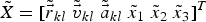 ${\tilde X} = [{\tilde {\vec r}}_{kl} \;{\tilde {\vec v}}_{kl} \;{\tilde {\vec a}}_{kl} \;{\tilde x}_1 \;{\tilde x}_2 \;{\tilde x}_3 ]^T $
, and
${\tilde X} = [{\tilde {\vec r}}_{kl} \;{\tilde {\vec v}}_{kl} \;{\tilde {\vec a}}_{kl} \;{\tilde x}_1 \;{\tilde x}_2 \;{\tilde x}_3 ]^T $
, and
 $${\tilde w}_l = - \displaystyle{{\,f_d} \over c}\left[ {\displaystyle{{({\tilde {\vec r}}_l - {\tilde {\vec r}}_k )^T ({\tilde {\vec v}}_l - {\tilde {\vec v}}_k )} \over {\sqrt {({\tilde {\vec r}}_l - {\tilde {\vec r}}_k )^T ({\tilde {\vec r}}_l - {\tilde {\vec r}}_k )}}}} \right]$$
Therefore, the new observation
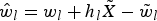 $\hat w_l = w_l + h_l \tilde X - \tilde w_l $
can be used to replace the estimated Doppler shift of the DSRC, w
l
, which is received from vehicle l. Then the observation vector can be defined as:
$\hat w_l = w_l + h_l \tilde X - \tilde w_l $
can be used to replace the estimated Doppler shift of the DSRC, w
l
, which is received from vehicle l. Then the observation vector can be defined as:
 $$Z = \left[ {\matrix{ {\rho _{kl}^{12}} \hfill & \cdots \hfill & {\rho _{kl}^{1m}} \hfill & {\vartheta _{kl}^{12}} \hfill & \cdots \hfill & {\vartheta _{kl}^{1m}} \hfill & {\vec a_{kl}^T} \hfill & {\hat w_l} \hfill \cr}} \right]^T $$
 $$\zeta = \left[ {\matrix{ {\zeta _{kl}^{12}} \hfill & \cdots \hfill & {\zeta _{kl}^{1m}} \hfill & {\gamma _{kl}^{12}} \hfill & \cdots \hfill & {\gamma _{kl}^{1m}} \hfill & {\vec \delta _{kl}^T} \hfill & {\varsigma _l} \hfill \cr}} \right]^T $$
where
 $\vec \delta _{kl} $
is IMU acceleration noise with the variance
$\vec \delta _{kl} $
is IMU acceleration noise with the variance
 $\sigma _a^2 $
that is mutually independent among three axes, and
$\sigma _a^2 $
that is mutually independent among three axes, and
 $\varsigma _l $
is the observation noise of Doppler shift of the DSRC. m is the number of GPS satellites commonly visible at vehicles k and l. The satellite with the highest elevation angle is chosen as the reference satellite (i.e. the first satellite) to be differenced against other satellites. According to Equations (4), (5), (9), (13), and (17)–(19), we have
$\varsigma _l $
is the observation noise of Doppler shift of the DSRC. m is the number of GPS satellites commonly visible at vehicles k and l. The satellite with the highest elevation angle is chosen as the reference satellite (i.e. the first satellite) to be differenced against other satellites. According to Equations (4), (5), (9), (13), and (17)–(19), we have
 $$H = \left[ {\matrix{ U \hfill & {{\it 0}_{(m - 1) \times 3}} \hfill & {{\it 0}_{(m - 1) \times 3}} \hfill & {{\it 0}_{(m - 1) \times 3}} \hfill \cr {{\it 0}_{(m - 1) \times 3}} \hfill & { - U\lambda ^{ - 1}} \hfill & {{\it 0}_{(m - 1) \times 3}} \hfill & {{\it 0}_{(m - 1) \times 3}} \hfill \cr {{\it 0}_3} \hfill & {{\it 0}_3} \hfill & {{\it I}_3} \hfill & {{\it 0}_3} \hfill \cr {H_1} \hfill & {H_2} \hfill & {{\it 0}_{1 \times 3}} \hfill & {{\it 0}_{1 \times 3}} \hfill \cr}} \right]$$
Where
 $$U(t) = \left[ {\matrix{ {\vec u_1^T (t) - \vec u_2^T (t)} \hfill \cr {\vec u_1^T (t) - \vec u_3^T (t)} \hfill \cr \hfill\vdots \hfill \cr {\vec u_1^T (t) - \vec u_m^T (t)} \hfill \cr}} \right]$$
 $$H_1 = \left[ {\matrix{ {h_{l1}} \hfill & {h_{l2}} \hfill & {h_{l3}} \hfill \cr}} \right]$$
 $$H_2 = \left[ {\matrix{ {h_{l4}} \hfill & {h_{l5}} \hfill & {h_{l6}} \hfill \cr}} \right]$$
 $$h_{l1} = \displaystyle{{\partial w_l} \over {\partial r_{kl}^x}} = \displaystyle{\,f \over c} \cdot \displaystyle{{r_{kl}^x (\vec r_l - \vec r_k )^T (\vec v_l - \vec v_k ) - v_{kl}^x (\vec r_l - \vec r_k )^T (\vec r_l - \vec r_k )} \over {\left( {(\vec r_l - \vec r_k )^T (\vec r_l - \vec r_k )} \right)^{\textstyle{3 \over 2}}}} $$
 $$h_{l2} = \displaystyle{{\partial w_l} \over {\partial r_{kl}^y}} = \displaystyle{\,f \over c} \cdot \displaystyle{{r_{kl}^y (\vec r_l - \vec r_k )^T (\vec v_l - \vec v_k ) - v_{kl}^y (\vec r_l - \vec r_k )^T (\vec r_l - \vec r_k )} \over {\left( {(\vec r_l - \vec r_k )^T (\vec r_l - \vec r_k )} \right)^{\textstyle{3 \over 2}}}} $$
 $$h_{l3} = \displaystyle{{\partial w_l} \over {\partial r_{kl}^z}} = \displaystyle{\,f \over c} \cdot \displaystyle{{r_{kl}^z (\vec r_l - \vec r_k )^T (\vec v_l - \vec v_k ) - v_{kl}^z (\vec r_l - \vec r_k )^T (\vec r_l - \vec r_k )} \over {\left( {(\vec r_l - \vec r_k )^T (\vec r_l - \vec r_k )} \right)^{\textstyle{3 \over 2}}}} $$
 $$h_{l4} = \displaystyle{{\partial w_l} \over {\partial v_{kl}^x}} = - \displaystyle{\,f \over c} \cdot \displaystyle{{r_{kl}^x} \over {\left( {(\vec r_l - \vec r_k )^T (\vec r_l - \vec r_k )} \right)^{\textstyle{1 \over 2}}}} $$
 $$h_{l5} = \displaystyle{{\partial w_l} \over {\partial v_{kl}^y}} = - \displaystyle{\,f \over c} \cdot \displaystyle{{r_{kl}^y} \over {\left( {(\vec r_l - \vec r_k )^T (\vec r_l - \vec r_k )} \right)^{\textstyle{1 \over 2}}}} $$
 $$h_{l6} = \displaystyle{{\partial w_l} \over {\partial v_{kl}^z}} = - \displaystyle{\,f \over c} \cdot \displaystyle{{r_{kl}^z} \over {\left( {(\vec r_l - \vec r_k )^T (\vec r_l - \vec r_k )} \right)^{\textstyle{1 \over 2}}}} $$
Assuming that observations are independent, then the observation noise covariance for
 $\varsigma $
can be expressed as
$\varsigma $
can be expressed as
 $$\Sigma = \left[ {\matrix{ {\Sigma _\rho} \hfill & {{\it 0}_{m - 1}} \hfill & {{\it 0}_{(m - 1) \times 3}} \hfill & 0 \hfill \cr {{\it 0}_{m - 1}} \hfill & {\Sigma _\vartheta} \hfill & {{\it 0}_{(m - 1) \times 3}} \hfill & 0 \hfill \cr {{\it 0}_{3 \times (m - 1)}} \hfill & {{\it 0}_{3 \times (m - 1)}} \hfill & {\Sigma _a} \hfill & 0 \hfill \cr {{\it 0}_{1 \times (m - 1)}} \hfill & {{\it 0}_{1 \times (m - 1)}} \hfill & {{\it 0}_{1 \times 3}} \hfill & {\Sigma _\omega} \hfill \cr}} \right]$$
Considering that the rotational matrix
 $C_b^n $
is orthogonal, the covariance of the acceleration noise for the navigation frame will also be
$C_b^n $
is orthogonal, the covariance of the acceleration noise for the navigation frame will also be
 $\sigma _a^2 I_3 $
. Therefore, the covariance of relative acceleration is
$\sigma _a^2 I_3 $
. Therefore, the covariance of relative acceleration is
 $\Sigma _a = 2\sigma _a^2 I_3 $
. The Doppler shift of the DSRC is considered to be a zero mean Gaussian with STD of σ
ω
, therefore
$\Sigma _a = 2\sigma _a^2 I_3 $
. The Doppler shift of the DSRC is considered to be a zero mean Gaussian with STD of σ
ω
, therefore
 $\Sigma _\omega = \sigma _\omega ^2 $
. We define
$\Sigma _\omega = \sigma _\omega ^2 $
. We define
 $\sigma _\rho ^2 $
and
$\sigma _\rho ^2 $
and
 $\sigma _\vartheta ^2 $
as the variance of the GPS pseudorange and the Doppler shift observation error, respectively. Subsequently, we have (Alam et al., Reference Alam, Kealy and Dempster2013b)
$\sigma _\vartheta ^2 $
as the variance of the GPS pseudorange and the Doppler shift observation error, respectively. Subsequently, we have (Alam et al., Reference Alam, Kealy and Dempster2013b)
 $\Sigma _\rho = \sigma _\rho ^2 AA^T $
and
$\Sigma _\rho = \sigma _\rho ^2 AA^T $
and
 $\Sigma _\vartheta = \sigma _\vartheta ^2 AA^T $
, where
$\Sigma _\vartheta = \sigma _\vartheta ^2 AA^T $
, where
 $$A = \left[ {\matrix{ {1_{(m - 1) \times 1}} \hfill & { - I_{(m - 1)}} \hfill & { - 1_{(m - 1) \times 1}} \hfill & {I_{(m - 1)}} \hfill \cr}} \right]$$
where 1 in A represents a matrix with subscripted dimensions and all entries 1. Having F, G, H, Q and Σ defined, the standard equations of the Extended Kalman Filter EKF) for the proposed tight CP method can now be implemented.
The tight CP with INS (Alam et al., Reference Alam, Kealy and Dempster2013b) also used the inertial data. Apart from using the DSRC Doppler in the new proposed method, another difference is that here, the Euler angles are introduced to the Kalman filter state variables as shown in Equations (14) to (22) instead of using GPS Doppler to estimate the Euler angles. Hence, this overcomes the restriction in Alam et al. (Reference Alam, Kealy and Dempster2013b) where the acceleration in the body frame cannot be accurately converted into the navigation frame because of GPS outage. Therefore, another INS-aided tight CP method using the same state space model, Equation (22), and the same observations shown in Equation (38) but without DSRC Doppler, can also be used for relative positioning. To distinguish it from the tight CP with INS method in Alam et al. (Reference Alam, Kealy and Dempster2013b), the method proposed here is named tight CP with IMU.
4. EXPERIMENTAL RESULTS
To evaluate the presented tight CP method, the same experimental data used in Alam et al. (Reference Alam, Kealy and Dempster2013b) is again used here. The experiment setup included two vehicles equipped with GPS receivers, INS and DSRC transceivers. Expensive reference equipment and a set of low cost sensors were fitted into each test vehicle. The type of DSRC transceiver is MK2 from CohdaWireless™. The equipment used to acquire reference position was the Leica GS10 geodetic RTK receiver for vehicle 1, and a Novatel INS-LCI (integrated GNSS-INS) for vehicle 2. The carrier-phase-based differential position estimates (RTK) of these receivers were used as ground truth position data. The noisy L1 pseudoranges, Doppler shifts, and low-cost MEMS IMU (Xsens Mti-G), and the Doppler DSRC-based readings were used as measurements for the tight CP algorithm proposed. Figure 3 shows a photograph of the two experiment vehicles. The sampling rate of experimental data was 1 Hz, and GPS time was used for data synchronisation. Therefore, the time delay for DSRC signal was ignored in our experiment.

Figure 3. Two experiment vehicles.
The duration of the entire experiment was much more than the 14 minutes of data selected; however, this was the largest continuous block of data with corresponding RTK GPS fixes. The performance of DGPS (Kaplan and Hegarty, Reference Kaplan and Hegarty2006), the tight CP (Alam et al., Reference Alam, Balaie and Dempster2013a), the tight CP with INS (Alam et al., Reference Alam, Kealy and Dempster2013b), the tight CP with IMU, and the tight CP with Doppler and IMU proposed in this paper are compared using the same experimental data. To describe conveniently, “DGPS”, “T-CP”, “T-CP with INS”, “T-CP with IMU” and “T-CP with Doppler and IMU” are used in the following figures and table to denote the five methods mentioned above.
The relative distance error of two vehicles, i.e.,
 $e_d (t) = \vert \vec r'(t) - \vec r(t)\vert$
, was calculated, where
$e_d (t) = \vert \vec r'(t) - \vec r(t)\vert$
, was calculated, where
 $\vec r'(t)$
and
$\vec r'(t)$
and
 $\vec r(t)$
are the estimated and the true relative position, respectively. In addition to the Root Mean Square (RMS) of e
d
, i.e., rmse, the accuracy and precision of relative positioning are evaluated. The performance of those methods are compared between two cases, GPS coverage and outage, respectively.
$\vec r(t)$
are the estimated and the true relative position, respectively. In addition to the Root Mean Square (RMS) of e
d
, i.e., rmse, the accuracy and precision of relative positioning are evaluated. The performance of those methods are compared between two cases, GPS coverage and outage, respectively.
4.1. Environments with GPS Availability
Figure 4 shows the number of common visible satellites for the vehicles for the experiment data. It can be seen that the number of common visible satellites is almost always above the required minimum, i.e., four. However, when it occasionally falls below the minimum, the Kalman filter can compensate by setting the innovation of the missing observation to zero and assigning a large number to the corresponding covariance of the missing observation.

Figure 4. Common Satellite visibility of the experimental data selected.
Table 1 summarises the performance indicators for the experimental results of the entire 14 minutes of data. It can be seen that the tight CP with Doppler and IMU proposed in this paper outperforms all other existing methods. The performance of tight CP with IMU is similar to tight CP with INS.
Table 1. Experimental results for relative positioning errors.

For performance comparison purposes,
 $(1 - ErrorB/ErrorA) \times 100\% $
is defined for demonstrating the percentage of improvement achieved over method A using method B. Table 2 summarises the experimental results of performance improvements achieved for different methods which shows that the proposed fusion of DSRC Doppler observations into the Tight CP integration has similar or better performance than existing Tight CP techniques.
$(1 - ErrorB/ErrorA) \times 100\% $
is defined for demonstrating the percentage of improvement achieved over method A using method B. Table 2 summarises the experimental results of performance improvements achieved for different methods which shows that the proposed fusion of DSRC Doppler observations into the Tight CP integration has similar or better performance than existing Tight CP techniques.
Table 2. Percentage improvements achieved.

To further evaluate the performance of the proposed method with different numbers of visible GPS satellites, we manually masked the GPS data with different visible satellites to emulate obstructions to low elevation satellites, which is more representative of dense urban scenarios (Chao et al., Reference Chao, qi Chen, Chen, Ding, Wong and Yu2001).
As shown in Figure 5, the maximum number of common visible satellites, m, adopts 7, and 6, and 5. Similar to the results in Table 2, it was verified that the tight CP with INS method outperforms the tight CP method and DGPS. In this scenario, we only compare two proposed methods, the tight CP with IMU, and the tight CP with Doppler and IMU proposed, against the best of the existing methods, which is the tight CP with INS method. Table 3 summarises the rmse for this experiment, and Table 4 gives the improvements achieved for relative positioning errors with different maximum number of common visible GPS satellites.

Figure 5. The simulation for different number of common visible GPS satellites.
Table 3. Experimental results for relative positioning errors.

Table 4. Improvements achieved for relative positioning errors.
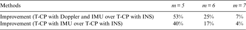
As can be seen, the proposed tight CP with Doppler and IMU outperforms tight CP with INS and the proposed tight CP with IMU. As the number of common visible satellites decreases, a higher factor of improvement is achieved. In addition, it can also be seen that the proposed tight CP with IMU outperforms the tight CP with INS. The reason is that the Euler angles do not rely on the GPS data in the tight CP with IMU solution. Therefore, the measurements of acceleration can also play a role in improving positioning performance in the low GPS coverage scenarios.
4.2. GPS Outage Scenario
As mentioned previously, in some circumstances such as dense urban areas and tunnels the chances of observing four common satellites by the vehicles is low. In severe circumstances, no GPS satellites can be observed (e.g. in a tunnel). To evaluate the performance of the proposed method in a GPS outage, the GPS data of four selected time segments were masked from the entire 14-minute data logged. That is, beginning at 100 s, 300 s, 500 s, and 700 s, the GPS measurements of all satellites are made unavailable, i.e. 100% outage. But the duration of GPS outage is varied between 1 s to 20 s to emulate a more general urban environment.
Figure 6 shows the rmse for different techniques as a function of satellite outage duration. As expected, the rmse considerably deteriorates with the increase in GPS outage duration, and the two proposed tight CP methods, tight CP with IMU and tight CP with Doppler and IMU, both outperform the other three methods significantly. This shows the significant resilience against GPS outage provided by the proposed DSRC Doppler-based solution. This can be attributed to the fact that the inter-vehicle Doppler observations suffer less from the random walk effect as opposed to the IMU observations. It can also been seen that because the INS-based accelerations depend on GPS Doppler measurements, the performance of the tight CP with INS degrades faster with the duration of GPS outage increased. On the contrary, the proposed tight CP with IMU produces smaller errors for all GPS outage durations than DGPS, and tight CP, and tight CP with INS.

Figure 6. Rmse of different techniques over GPS outage periods.
Figure 7 gives the position accuracy of different methods under the GPS outage scenario. It can be seen that the two proposed methods have higher position accuracy than the other three methods. Comparing with the proposed method without DSRC, a little improvement is achieved with the proposed method with DSRC. Also, it shows the performance deterioration of “T-CP with INS” to be worse than “T-CP” over outage time. This is the repercussion of relying on GPS Doppler for calculating the body frame to navigation frame rotation matrix. The method adopted in our paper circumvents this artefact as shown by “T-CP with IMU (proposed)” and “T-CP with Doppler and IMU (proposed)”.

Figure 7. Accuracy of different methods over GPS outage periods.
Figure 8 shows the rmse improvement achieved as a function of satellite outage duration. The performance improvement achieved by the proposed T-CP with Doppler and IMU solution over tight CP with IMU, tight CP with INS, tight CP and DGPS, are up to 40%, 60%, 55%, and 66%, respectively. Also, as shown in Figure 8, the performance of tight CP with INS degrades faster than the three other methods. When the GPS outage is more than 14 seconds, the performance of tight CP with INS is observed to be worse than tight CP. Contrarily, it can be seen in Figures 6, 7 and 8 that the proposed tight CP with IMU always outperforms the tight CP with INS, and tight CP, and DGPS as a result of utilising a tight integration approach and filtered Euler angles.

Figure 8. Rmse improvement achieved over GPS outage periods.
Figure 9 shows the rmse as a function of the relative velocity of two vehicles in the select duration of GPS outage. The two proposed methods and the method of tight CP with INS are compared here, in which the rmse have the same trend as the relative speed.

Figure 9. The rmse of different methods with different relative speed during the GPS outage.
5. CONCLUSION
A tight integration Cooperative Positioning (CP) technique is proposed for relative positioning in VANETs, which is based on fusing GPS data, IMU data, and DSRC-based inter-vehicular Doppler data from participating neighbouring vehicles. The functionality and performance of the proposed method has been verified and compared against three recent existing CP methods, namely DGPS, tight CP, and tight CP with INS. The experiment shows that with full GPS coverage, the proposed CP method outperforms existing methods. At worst, the method's improvement in precision of approximately 6%, 15%, and 28% is observed when compared against tight CP with INS, tight CP and DGPS, respectively. In limited satellite visibility conditions, the performance improvements delivered by the proposed methods are even more significant due to the utility of neighbouring DSRC and IMU measurements. In GPS outage scenarios, performance improvement of up to 60%, 55%, and 66% in rmse is achievable compared against the existing tight CP methods. Therefore, the proposed tight CP method can effectively enhance the performance of relative positioning especially in low GPS visibility and GPS outages, which is typical of very dense urban areas and tunnels.
It also should be noted that there is still a gap between the available results and the desired performance for safety-critical applications such as collision avoidance during GPS outages. However, other sensors such as radars, digital maps, odometer and cameras can also be used and this represents future work.
ACKNOWLEDGMENT
The authors would like to thank Associate Professor A. Kealy from the Department of Infrastructure Engineering, University of Melbourne, Parkville, Australia, Doctors C. Hill and S. Ince from the Nottingham Geospatial Institute, University of Nottingham, Nottingham, U.K., and for their support and collaboration in the experiments conducted for this work. Meanwhile, this work was supported by National Nature Science Foundation of China under grants 61102107 and 61374208.


