


1. Introduction
A variation of viscosity in space and time occurs in a vast range of flows. Practically all flows where composition or temperature are not constant are of varying viscosity. Changes in viscosity are known to affect the stability of the flow dramatically. While an enormous literature is available on viscosity stratification and its effect on linear instability, far less is studied about how it impacts the non-modal growth of perturbations. Understanding the transition to turbulence in shear flow requires understanding how non-modal perturbations grow and propagate. In recent years, it has been recognised (Cherubini et al. Reference Cherubini, De Palma, Robinet and Bottaro2010; Pringle & Kerswell Reference Pringle and Kerswell2010; Pringle, Willis & Kerswell Reference Pringle, Willis and Kerswell2012) that studying the nonlinear optimal perturbations is essential to this effort. The present study is the first to our knowledge on nonlinear optimal perturbations in viscosity-stratified flows. Our interest is in a gentle variation of viscosity rather than a sharp one, and we choose a pressure-driven channel flow with the walls maintained at different temperatures as a prototypical model flow to reveal the essential physics. Further, we are interested in short term optimisation, to underline how viscosity-varying flows already depart considerably from constant-viscosity flows. We set gravity to zero in this study to isolate the effects of viscosity variation.
The interaction of viscosity stratification and shear can lead to both suppression and enhancement of flow instabilities (for a review, see Govindarajan & Sahu Reference Govindarajan and Sahu2014). A viscosity jump across an interface can give rise to linear instability at any Reynolds number (e.g. see Yih Reference Yih1967). On the other hand, a lowering of viscosity near a wall has been studied for decades as a means to stabilise shear flow and to thus achieve drag reduction, e.g. in lubricating oil pipelines (Preziosi, Chen & Joseph Reference Preziosi, Chen and Joseph1989). Composition variation and the introduction of polymers, whence besides elasticity, viscosity stratification resulting due to shear thinning can be important, have been explored over the years. In aerospace applications (Mack Reference Mack1984), a viscosity reduction near the wall in a boundary layer can provide a fuller and more stable velocity profile. By virtue of viscosity (e.g. see Schmid, Henningson & Jankowski Reference Schmid, Henningson and Jankowski2002) and its spatial gradients (Govindarajan Reference Govindarajan2004) being multiplied by the highest derivatives in the stability equations, we are presented with a singular perturbation problem. In other words, however high the Reynolds number (however small the viscosity), viscosity and its variations can have a large effect on the flow. For example, Ranganathan & Govindarajan (Reference Ranganathan and Govindarajan2001) showed that a ten per cent change in viscosity across a thin layer can, if overlapped with the critical layer of the least stable eigenmode, give rise to an order of magnitude change in the critical Reynolds number  $Re_c$ of $5772.2$ in a channel. The effect of wall heating and subsequent viscosity changes on a fully developed turbulent flow has been studied using direct numerical simulations (DNS) for both a boundary layer (Lee et al. Reference Lee, Jung, Sung and Zaki2013) and a channel flow (Zonta, Marchioli & Soldati Reference Zonta, Marchioli and Soldati2012). Zonta et al. (Reference Zonta, Marchioli and Soldati2012) find vortical structures to be more populated near the colder (more-viscous) wall as compared to the hotter (less-viscous) wall, while Lee et al. (Reference Lee, Jung, Sung and Zaki2013) find that vortical structures near the heated wall are unaffected, whereas away from the wall, they become sparser with wall heating. The effects of a continuous variation of viscosity have also been investigated in the linear stability studies of Potter & Graber (Reference Potter and Graber1972), Schäfer & Herwig (Reference Schäfer and Herwig1993), Wall & Wilson (Reference Wall and Wilson1996) and Sameen & Govindarajan (Reference Sameen and Govindarajan2007).
For a channel flow below  $Re_c$, a traditional normal-mode analysis predicts that the energy of no single eigenmode can grow in isolation. However, the linear stability operator of the flow, obtained by linearising the Navier–Stokes equations about a laminar flow and posing the resulting Orr–Sommerfeld and Squire equations as an eigenvalue problem, is non-normal. Hence, a transient (algebraic) growth in energy can occur in the flow due to the superimposition of suitably arranged eigenmodes at intermediate time (Reddy & Henningson Reference Reddy and Henningson1993; Trefethen et al. Reference Trefethen, Trefethen, Reddy and Driscoll1993). Shear makes the governing operator non-normal and transient growth is experienced, for example, in channel flow, pipe flow and Couette flow. If the transient growth is large enough, nonlinear mechanisms could be activated. It is now accepted that findings such as that the transition to turbulence in a channel at $Re\approx 1000$ (e.g. Orszag & Patera Reference Orszag and Patera1980; Carlson, Widnall & Peeters Reference Carlson, Widnall and Peeters1982) are a manifestation of these non-modal and nonlinear mechanisms. For such flows, non-modal analyses complement modal analysis in fully understanding the behaviour (Böberg & Brosa Reference Böberg and Brosa1988; Butler & Farrell Reference Butler and Farrell1992; Trefethen et al. Reference Trefethen, Trefethen, Reddy and Driscoll1993; Trefethen & Embree Reference Trefethen and Embree2005) (for a review, see Schmid Reference Schmid2007). A linear non-modal study often optimises for the energy growth of an infinitesimal initial perturbation over all possible initial conditions, and from the singular value decomposition (SVD) of the linear operator, reveals the optimal perturbation, i.e. the initial perturbation that leads to the largest transient growth in the linear regime.
For any amplitude of initial perturbation, the optimal perturbation can be obtained by an adjoint-based iterative optimisation procedure with the full, or linearised, Navier–Stokes equations as in Schmid (Reference Schmid2007). The procedure would be the same for linearised or nonlinear equations. Also, the nonlinear equations could be used along with a very small disturbance amplitude to yield effectively linear solutions. This procedure involves repeated computations of adjoint fields and the sensitivity of a cost functional to changes in the initial perturbation. It has been applied to the Navier–Stokes equations for control of fluid flow by Abergel & Temam (Reference Abergel and Temam1990), Bewley, Temam & Ziane (Reference Bewley, Temam and Ziane2000), Corbett & Bottaro (Reference Corbett and Bottaro2000) and Zuccher, Luchini & Bottaro (Reference Zuccher, Luchini and Bottaro2004) among others, and to numerically calculate the optimal perturbations and the associated transient growth, within the framework of the linearised as well as of the nonlinear Navier–Stokes equations, as in Monokrousos et al. (Reference Monokrousos, Bottaro, Brandt, Di Vita and Henningson2011), Foures, Caulfield & Schmid (Reference Foures, Caulfield and Schmid2013), Kaminski, Caulfield & Taylor (Reference Kaminski, Caulfield and Taylor2014), Marcotte & Caulfield (Reference Marcotte and Caulfield2018) and Vermach & Caulfield (Reference Vermach and Caulfield2018) (for a review, see Kerswell (Reference Kerswell2018)). The nonlinear optimal perturbation has been found to have a different spatial structure from the linear optimal perturbation (Rabin, Caulfield & Kerswell Reference Rabin, Caulfield and Kerswell2012). Since the full nonlinear equations are optimised, the nonlinear optimal perturbation leads to a larger transient growth (Cherubini et al. Reference Cherubini, De Palma, Robinet and Bottaro2010; Pringle & Kerswell Reference Pringle and Kerswell2010; Luchini & Bottaro Reference Luchini and Bottaro2014). This hints at the importance of the nonlinearity in the non-modal analysis and indicates that the search for a minimal seed for turbulence onset must involve studying the time evolution of the nonlinear optimal (e.g. see Pringle et al. Reference Pringle, Willis and Kerswell2012).
In this paper, we investigate the sole effects of viscosity stratification on the optimal perturbation and the resultant transient growth at early times. Our central idea is to investigate how the process of subcritical perturbation growth in the nonlinear regime is affected by viscosity variations. We consider the full nonlinear Navier–Stokes equations, modified to account for varying viscosity, and derive the adjoint viscosity-stratified Navier–Stokes equations. We then formulate a nonlinear stability theory using the adjoint-based optimisation technique. We utilise this framework to calculate the optimal perturbation for a certain fixed target time. Performing studies with very small and more significant initial perturbation amplitudes, our findings show how nonlinearity is a crucial part of the initial evolution, although the Orr and lift-up mechanisms in operation have linear underpinnings. The evolution of initial perturbation which maximises linear energy growth is restricted to the hot wall, whereas optimising for nonlinear energy growth shows how the cold wall is more important, with persistent streaks and velocity profiles becoming increasingly inflectional.
2. Governing equations and problem formulation
We study pressure-driven flow through a three-dimensional channel bounded by two parallel walls, kept fixed at  $y = {\pm }L_y$ as depicted in figure 1. The mean pressure gradient $\textrm {d}P/{\textrm {d}\kern0.05em x}$ forces the flow in the $x$ direction. Hence, $x$ is the streamwise direction and $z$ the spanwise direction. The temperature of both walls is kept constant, with the wall at $y = +L_y$ at a higher temperature than the wall at $y = -L_y$. There is no gravity in this problem, and non-Boussinesq effects arising from density change due to temperature variations are neglected. The half-width, $L_y$, of the channel is chosen as our length scale. The non-dimensional size of the channel is fixed at $2{\rm \pi} , 2$ and ${\rm \pi}$ in the $x$,
$x$,  $y$ and $z$ directions, respectively.

Figure 1. The flow domain being studied. The flow is from left to right, driven by the mean pressure gradient  $\textrm {d}P/{\textrm {d}\kern0.05em x}$. Here, $L_x = 2{\rm \pi} L_y$ is the streamwise length, $L_z = {\rm \pi}L_y$ is the spanwise length and $L_y$ is the half-width of the channel. The hot and cold walls at $y = {\pm }L_y$ are kept at constant but different temperatures.
The unperturbed laminar flow through the channel is our base state. Three-dimensional perturbations are introduced over this base state. The non-dimensional governing equations for a viscosity-stratified flow read as
 \begin{gather} \frac{\partial u_i}{\partial x_i}=0, \end{gather}
 \begin{gather} \frac{\partial{u_i}}{\partial{t}}+(U_j+u_j)\frac{\partial u_i}{\partial x_j} +u_j\frac{\partial U_i}{\partial x_j}={-}\frac{\partial p}{\partial x_i}+{\frac{2 \beta}{Re}}{\frac{\partial}{\partial x_j}} [{\mu}(s_{ij}+S_{ij})+\bar{\mu}s_{ij}],\end{gather}
 \begin{gather} \frac{\partial{T}}{\partial{t}}+(U_j+u_j)\frac{\partial T}{\partial x_j} +u_j\frac{\partial(\bar{T}+T_0)}{\partial x_j}=\frac{1}{{Re }Pr} \frac{\partial^2T}{\partial x_j^2}.\end{gather}
Here,  $U_j =\delta _{j1} U(\kern-0.004em y)$ is the laminar base state, consisting only of a streamwise component, $u_j(x,y,z,t)$ are the components of the perturbation velocity $\boldsymbol {u}(\boldsymbol {x},t)$ and $p(\boldsymbol {x},t)$ is the perturbation pressure; $x, y$ and $z$ are referred to as $x_1$, $x_2$ and $x_3$, respectively,
 \begin{equation} S_{ij} = \frac{1}{2} \left( \frac{\partial U_i}{\partial x_j}+\frac{\partial U_j}{\partial x_i} \right) \quad \text{and} \quad s_{ij} = \frac{1}{2} \left( \frac{\partial u_i}{\partial x_j}+\frac{\partial u_j}{\partial x_i} \right) \end{equation}
are the base and the perturbation velocity strain tensors, respectively. The parameter  $T(\boldsymbol {x},t)$ is the perturbation temperature, and the base state temperature $\bar {T}(\kern-0.004em y)+T_0$ is linear in $y$, varying from the reference temperature $T_0$ at the bottom wall to $T_0 + \Delta T$ at the top wall. The base and perturbation viscosities, $\bar {\mu }(T)$ and $\mu (T)$ respectively, are functions of temperature alone, and are defined in § 2.1. The Reynolds number $Re$ and the viscosity ratio $\beta$ are defined in § 2.2. The parameter $Pr= \mu _{0} c_p/\rho k$ is the Prandtl number, where $\mu _{0}$ is the viscosity at the reference temperature $T_0$, $c_p$ the specific heat at constant pressure and $k$ the thermal conductivity of the fluid. The density $\rho$ of the fluid is taken to be a constant.
Barring the mean pressure drop, all variables of the flow are prescribed to be periodic at the domain boundaries in  $x$ and $z$. No-slip velocity boundary conditions are imposed at the walls.
We will refer to (2.2) as the modified Navier–Stokes equation, valid for viscosity-stratified flow. Equations (2.1)–(2.3) are referred to as the ‘direct’ equations to distinguish them from other equations, called the ‘adjoint’ equations, to be introduced in § 2.3. The variables appearing in (2.1)–(2.3) will be called direct variables. The initial velocity and temperature conditions are represented as  $\boldsymbol {u}(\boldsymbol {x},0) = \boldsymbol {u_0}(\boldsymbol {x})$ and $T(\boldsymbol {x},0)$.
2.1. Viscosity model and the base state
The local non-dimensional viscosity  $\mu _{tot}$ in the flow is modelled as an exponential function of the total temperature $T_{tot} = \bar T(\kern-0.004em y)+T_0 + T$, following Wall & Wilson (Reference Wall and Wilson1996), as
 \begin{equation} \mu_{tot} \equiv \bar{\mu} + \mu = \frac{\exp(-\kappa T_{tot})}{\exp(-\kappa T_0)}, \end{equation}
where
 \begin{equation} \bar{\mu}=\frac{\exp[-\kappa (\bar{T}(\kern-0.004em y)+T_0)]}{\exp(-\kappa T_0)}. \end{equation}
The viscosity of the cold wall is used as the scale here. With the constant  $\kappa$ chosen to be 0.012 per degree Kelvin, this function closely follows the viscosity of water in our temperature range. Since the density of water varies by less than 2 parts in a 1000 for the largest temperature difference, variations in kinematic viscosity are mainly from changes in dynamic viscosity. As is typical of liquids, the viscosity decreases with an increase in temperature, as shown in figure 2(a). The laminar base profile of the streamwise velocity given by Wall & Wilson (Reference Wall and Wilson1996) is
 \begin{equation} U(\kern-0.004em y) = \frac{-2 \alpha}{\kappa\Delta{T}}\left[1 + \coth \kappa\Delta{T} + (\kern-0.004em y - \coth \kappa\Delta{T})\exp(\kappa\Delta{T}(1+y)) \right], \end{equation}
where
 \begin{equation} \alpha=\frac{2\kappa\Delta T}{3}\frac{1}{-2(1+\coth{\kappa\Delta T})+(\exp(2\kappa\Delta T)-1)/(\kappa\Delta T)^3}, \end{equation}
allows for the same non-dimensional volumetric flow rate through the channel for different  $\Delta T$, as shown in figure 2(b).

Figure 2. (a) The wall-normal ( $y$) profiles, for various temperature differences $\Delta T$ between the walls, of base viscosity $\bar {\mu }(\kern-0.004em y)$ as given by (2.5b). The profile for $\Delta T = 0$ is a vertical line at $\bar {\mu }(\kern-0.004em y) = 1$. The ratios of viscosity between the top (hot) and the bottom (cold) wall are $0.61$ for $\Delta T = 20\ \textrm {K}$ (dashed line), $0.38$ for $\Delta T = 40\ \textrm {K}$ (dash-dotted line) and $0.23$ for $\Delta T = 60\ \textrm {K}$ (dotted line). (b) The unperturbed streamwise laminar velocity $U(\kern-0.004em y)$, normalised to have equal volumetric flux through the channel, for unstratified case (solid line) and different $\Delta T$.
2.2. The Reynolds number
In order to make a fair comparison between the growth of perturbation energy in a stratified flow and an unstratified flow, a careful definition of the Reynolds number is required. Note that when we refer to ‘unstratified’ flow, we mean constant-viscosity flow, and when we refer to ‘stratified’ flow, we mean a viscosity-stratified flow. As the laminar base velocity profile in a stratified channel is asymmetric around  $y=0$ (figure 2b), the centreline velocity is not a standard velocity scale across different stratification levels, whereas the volume flux is. Secondly, the viscosity in the channel decreases continuously when moving away from the cold wall at $y=-1$ (figure 2a). If, for example, $Re$ was defined based only on the viscosity at the cold wall, then the effective Reynolds number of the stratified channel would be higher than this value, and consequently, the perturbation energy growth could be expected to be higher. So, we choose the space-averaged mean viscosity as our viscosity scale to define $Re$. The Reynolds number used in this paper is
 \begin{equation} Re \equiv \rho L_y \frac{\displaystyle \int_{{-}L_y}^{L_y} 1.5 U(\kern-0.004em y)\,{\textrm{d}y}}{\displaystyle \int_{{-}L_y}^{L_y} \bar{\mu}_d\, {\textrm{d}y}} = \frac{1.5 \rho L_y \langle U\rangle}{\langle\bar{\mu}_d\rangle}, \end{equation}
where  $\bar {\mu }_d(T)$ is the dimensional base viscosity of the fluid, and the angle brackets represent an average in the wall-normal direction $y$. A factor of 1.5 is incorporated for ease of comparison with earlier studies on unstratified flow which use the centreline velocity as the velocity scale. The dimensional viscosity must therefore be scaled by the average viscosity in the channel, but for ease of comparison, we have scaled it by its value at the cold wall. This is adjusted for, by the introduction in (2.2) and (2.10) of the viscosity ratio
 \begin{equation} \beta = \frac{\bar{\mu}_d(T_0)}{\langle\bar{\mu}_d\rangle}. \end{equation}
In this paper, we remain in the subcritical regime by fixing  $Re$ at 500, which also allows for validation against the unstratified channel flow result of Vermach & Caulfield (Reference Vermach and Caulfield2018). The non-dimensional mean pressure gradient is constant in the streamwise direction and is given by
 \begin{equation} \frac{\textrm{d}P}{\textrm{d}\kern0.05em x}={-}\frac{2\alpha\beta}{Re}. \end{equation}
2.3. Non-modal analysis using ‘direct-adjoint looping’
The nonlinear non-modal analysis is formulated in terms of an optimisation procedure termed ‘direct-adjoint looping’ (Luchini & Bottaro Reference Luchini and Bottaro1998; Andersson, Berggren & Henningson Reference Andersson, Berggren and Henningson1999; Corbett & Bottaro Reference Corbett and Bottaro2000; Juniper Reference Juniper2011; Arratia, Caulfield & Chomaz Reference Arratia, Caulfield and Chomaz2013; Foures, Caulfield & Schmid Reference Foures, Caulfield and Schmid2014; Kaminski, Caulfield & Taylor Reference Kaminski, Caulfield and Taylor2017; Vermach & Caulfield Reference Vermach and Caulfield2018), to find the largest non-modal energy growth and the optimal perturbation of the flow that causes this growth. To effect this, we need to define a cost functional which includes some measure of energy, and the aim of the optimisation procedure would be to maximise this cost functional. Especially when density or viscosity or any flow component varies with space and time, there are many choices that may be made for the cost functional, and each choice could lead to a different optimal perturbation. For example, Foures et al. (Reference Foures, Caulfield and Schmid2014) show, interestingly, that energy optimisation leads to weak mixing, but optimal perturbations obtained from mixing optimisation are very effective in mixing, although evolving to lower energies. Monokrousos et al. (Reference Monokrousos, Bottaro, Brandt, Di Vita and Henningson2011) prescribe the time-averaged viscous dissipation of energy as their cost functional to understand laminar–turbulence transition in a Couette flow. They optimise the nonlinear equations for long optimisation times and search across various initial energy levels to find the least energetic initial condition that initiates this transition. Thus the aims of each study are critical in choosing an appropriate cost functional.
In this first attempt to understand the optimal perturbations in a viscosity-stratified channel flow, we study the growth of kinetic energy of the velocity perturbations. As noted in previous studies (Foures et al. Reference Foures, Caulfield and Schmid2014; Vermach & Caulfield Reference Vermach and Caulfield2018), perturbations growing through a given time horizon may not have the largest energy precisely at a target time. To account for this, we choose the ratio of the integral over time, up to a preset target time, of the perturbation kinetic energy, to the initial perturbation kinetic energy, as our cost functional. The time-integrated perturbation kinetic energy of the flow up to the target time  $\mathcal {T}$ is defined as
 \begin{equation} G(\mathcal{T}) = \frac{\gamma}{2} \int_{0}^{\mathcal{T}} \|\boldsymbol{u}(\boldsymbol{x},t)\|_{\mathcal{V}}^{2}\,\textrm{d}t, \end{equation}
where  $\|\boldsymbol {u}(\boldsymbol {x},t)\|_{\mathcal {V}}$ is the total (integrated over the channel volume $\mathcal {V}$) $L^2$-norm of the velocity perturbations $\boldsymbol {u}(\boldsymbol {x},t)$. Note that the math-calligraphy symbol $\mathcal {T}$ for the target time is distinguished from the italics $T$ for temperature. Here, $\gamma$ is a constant with units of inverse time, and has been set to unity throughout this study; $\mathcal {T}$ is non-dimensionalised with the advective time scale, i.e. $L_y/1.5\langle U \rangle$, a constant across the various stratification levels studied here. Time integration includes effects from the intermediate-time dynamics of the flow as opposed to just the energy at the target time $\mathcal {T}$. The other quantity needed to construct the cost functional is the total initial perturbation kinetic energy
 \begin{equation} E_0 = \tfrac{1}{2} \|\boldsymbol{u_0}(\boldsymbol{x})\|_{\mathcal{V}}^{2}. \end{equation}
The cost functional  $\mathcal {J}(\mathcal {T})$ of interest is
 \begin{equation} \mathcal{J}({\mathcal{T}}) = \frac{G({\mathcal{T}})}{E_{0}}. \end{equation}
Our aim is to find the optimal perturbation  $\boldsymbol {u_0}(\boldsymbol {x},0)_{opt}$ which maximises the cost functional
 \begin{equation} \mathcal{J}_{opt}({\mathcal{T}}) \equiv \mathcal{J}_{max}({\mathcal{T}}) = \frac{G_{opt}({\mathcal{T}})}{E_{0}}, \end{equation}
with a fixed initial energy  $E_0$. To effect this, we formulate the optimisation procedure by defining a Lagrangian $\mathcal {L}$, an augmented functional which contains the cost functional $\mathcal {J}({\mathcal {T}})$ in (2.13), constrained by the incompressibility condition (2.1), the modified viscosity-stratified Navier–Stokes equation (2.2), the temperature equation (2.3) and the initial velocity conditions of the flow. The constrained Lagrangian $\mathcal {L}$ is
 \begin{align} \mathcal{L}&=\mathcal{J}({\mathcal{T}})-\left[\frac{\partial{u_i}}{\partial{t}}+(U_j+u_j)\frac{\partial u_i}{\partial x_j} +u_j\frac{\partial U_i}{\partial x_j}+\frac{\partial p}{\partial x_i}-{\frac{2\beta}{Re}}{\frac{\partial}{\partial x_j}}({\mu}(s_{ij}+S_{ij})+\bar{\mu}s_{ij}),v_i\right]\nonumber\\ &\quad -\left[\frac{\partial{T}}{\partial{t}}+(U_j+u_j)\frac{\partial T}{\partial x_j} +u_j\frac{\partial(\bar{T}+T_0)}{\partial x_j}-\frac{1}{{Re }Pr} \frac{\partial^2T}{\partial x_j^2},\tau\right]\nonumber\\ &\quad -\left[\frac{\partial u_i}{\partial x_i},q\right]-\langle\langle u_i(0)-u_{0,i},v_{0,i}\rangle\rangle, \end{align}
where
 \begin{equation} {\langle\langle \boldsymbol{a},\boldsymbol{b} \rangle\rangle \equiv \frac{1}{\mathcal{V}}\int_{\mathcal{V}} a_ib_i\,\textrm{d}V} \end{equation}
is the normalised volume integral of the inner product of the vectors  $\boldsymbol {a} (\boldsymbol {x}, t)$ and $\boldsymbol {b} (\boldsymbol {x}, t)$, and
 \begin{equation} {[\boldsymbol{a},\boldsymbol{b}] \equiv \frac{1}{\mathcal{T}\mathcal{V}}\int_{0}^{\mathcal{T}}\int_{\mathcal{V}} a_ib_i \,\textrm{d}V\,\textrm{d}t} \end{equation}
is the normalised time integral of  $\langle \langle \boldsymbol {a},\boldsymbol {b} \rangle \rangle$. The constraints on the Lagrangian are imposed with the help of time- and/or space-varying Lagrange multipliers, which are our adjoint variables. Three of the constraints in (2.15) appear as the inner products of the governing equations for the conservation of momentum, temperature and mass, respectively, with the adjoint variables $v_i$, $\tau$ and $q$. In (2.15), $u_i(0)=u_{0,i}$ are the components of the initial perturbation velocity $\boldsymbol {u_0}(\boldsymbol {x})$. The constraint on the initial condition appears as its inner product with $v_{0,i}$, and its relevance will become apparent below. The adjoint velocity $v_i$, the adjoint temperature $\tau$, the adjoint pressure $q$ and the adjoint velocity initial condition $v_{0,i}$ correspond respectively to the direct variables $u_i$, $T$,
$T$,  $p$ and $u_{0,i}$.
The variation of  $\mathcal {L}$ with respect to all the variables and their corresponding adjoints are independent of each other. At the maximum of the cost functional $\mathcal {J}({\mathcal {T}})$ and hence $\mathcal {L}$ in (2.15), the variational derivatives identically vanish. The variation of $\mathcal {L}$ with respect to $p$ is discussed briefly here for illustration. Using integration by parts in three dimensions, we have
 \begin{equation} \frac{\delta \mathcal{L}}{\delta p} = \frac{1}{\mathcal{T}\mathcal{V}} \int_{0}^{\mathcal{T}}\int_{\mathcal{V}} v_i \frac{\partial\delta p}{\partial x_i} \,\textrm{d}V\,\textrm{d}t = \frac{1}{\mathcal{T}\mathcal{V}} \int_{0}^{\mathcal{T}} \left(\oint_{\mathcal{S}} v_i\delta p n_i\,\textrm{d}S - \int_{\mathcal{V}} \frac{\partial v_i}{\partial x_i} \delta p\,\textrm{d}V \right) \,\textrm{d}t, \end{equation}
where  $S$ is the surface enclosing the volume $\mathcal {V}$ and $n_i$ is the outward-pointing unit normal on the surface; $\delta p$ must be periodic at the domain boundaries of the homogeneous directions to ensure that the mean pressure drop $\textrm {d}P/{\textrm {d}\kern0.05em x}$ is constant. Hence, the requirement that the derivative on the left-hand side of (2.18) should vanish gives the incompressibility condition for the adjoint velocity
 \begin{equation} \frac{\partial v_i}{\partial x_i}=0. \end{equation}
Derivatives with respect to  $u_i$ and $T$ are treated similarly (for a detailed derivation with constant viscosity see Luchini & Bottaro (Reference Luchini and Bottaro2014) and Foures et al. (Reference Foures, Caulfield and Schmid2014)) to give the adjoint evolution equations (2.20) and (2.21) for $v_i$ and $\tau$ and the values of $v_i$ and $\tau$ at $t=\mathcal {T}$,
 \begin{gather} \frac{\partial v_i}{\partial t}- v_j\frac{\partial (u_j+U_j)}{\partial x_i}+\frac{\partial (v_i(U_j+u_j))}{\partial x_j}+\frac{\beta}{Re}\frac{\partial}{\partial x_j}\left[({\mu}+\bar{\mu})\left(\frac{\partial v_i}{\partial x_j}+\frac{\partial v_j}{\partial x_i}\right)\right]\nonumber\\ -\tau\frac{\partial (T+\bar{T}+T_0)}{\partial x_i}+\frac{\partial q}{\partial x_i}+\gamma u_i=0, \end{gather}
 \begin{gather} \frac{\partial \tau}{\partial t}+(U_j+u_j)\frac{\partial \tau}{\partial x_j}+\frac{1}{RePr}\frac{\partial^2\tau}{\partial x_j^2}-\frac{2\beta}{Re}\left[\frac{\partial\mu}{\partial T}\left(s_{ij}+S_{ij}\right)+\frac{\partial\bar{\mu}}{\partial T}s_{ij}\right]\frac{\partial v_i}{\partial x_j}=0, \end{gather}
 \begin{gather} v_i(\mathcal{T})=0, \quad \tau(\mathcal{T})=0. \end{gather}
The derivation also leads to the boundary conditions for the adjoint variables which are same as that of the direct variables.
Similarly, the derivatives of  $\mathcal {L}$ in (2.15) with respect to the adjoint variables give us back the direct equations (2.1)–(2.3) and the condition $u_i(0)=u_{0,i}$ for the initial velocity. We thus reconfirm that adjoint variables are essentially Lagrange multipliers. Equations (2.19)–(2.21) are the adjoint equations corresponding to the direct equations (2.1)–(2.3). We note that the adjoint equations are linear in the adjoint variables. The nonlinearity appears in terms of the direct variables which appear in both direct and adjoint equations. For a constant-viscosity flow, these adjoint equations reduce to those derived by Vermach & Caulfield (Reference Vermach and Caulfield2018) for mixing of a passive scalar. Here, $v_i$ and $q$ have the same dimensions as the direct variables $u_i$ and $p$ but $\tau$ behaves as the square of a velocity per unit temperature. Nevertheless, we refer to τ as the adjoint temperature since its evolution equation (2.21) is derived by taking a variation of $\mathcal {L}$ in (2.15) with respect to temperature $T$. We notice that, in the absence of viscosity stratification, the last term in (2.21), with the coefficient of $2\beta /Re$, vanishes, and since we have no gravity, the solution to (2.21) is just $\tau =0$, and the temperature term will drop out of the adjoint momentum equation (2.20). The signs of the diffusion of adjoint momentum and temperature in (2.20) and (2.21) imply that, only during backward time evolution, i.e. from $t=\mathcal {T}$ to 0, are these equations well-posed. We also have in (2.22a,b) the required ‘initial’ conditions for $v_i$ and $\tau$ at $t=\mathcal {T}$ for the backward marching. Hence, a loop in time can be set up. At the very first iteration, we start with a guess of the optimal perturbation $\boldsymbol {u_0}(\boldsymbol {x})_{opt}$. In our case, this is a random noise. The temperature perturbations are set to zero at $t=0$. The direct equations (2.1)–(2.3) are marched forward in time until $t=\mathcal {T}$, where the adjoint variables are initialised according to (2.22a,b). The adjoint equations (2.19)–(2.21) are marched backwards in time from $t=\mathcal {T}$ to 0 (note that they are well-posed only in this direction). We then update $\boldsymbol {u_0}(\boldsymbol {x})$ for the next iteration by moving it in the direction provided by the variational derivative $\delta \mathcal {L}/\delta \boldsymbol {u_0}(\boldsymbol {x})$, which takes us closer to the optimal perturbation (and hence increases the objective functional). Another constraint that is missing in (2.15) is the imposition of a fixed $E_0$, a crucial component in this nonlinear optimisation. In the case of linearised equations, this would not be a necessity as the initial perturbation energy for the optimisation purpose could be arbitrarily set to unity. This initial energy constraint could have been imposed with a Lagrange multiplier in (2.15), but that has been found to be numerically expensive and delicate (Foures et al. Reference Foures, Caulfield and Schmid2013). Hence, during the update of the initial perturbation, carried out to march towards the optimal perturbation based on the gradient information, we use a rotation technique to constrain the $E_0$ of the updated perturbation on a fixed energy hypersphere, as described in detail in Foures et al. (Reference Foures, Caulfield and Schmid2013). The adjoint equations for a viscosity-stratified flow are derived here for the first time to our knowledge. We see new terms involving gradients in viscosity, both of the mean and of the perturbations, entering the adjoint velocity as well as the adjoint temperature equations.
As mentioned, the temperature perturbations are initially set to zero for the evolution of the direct equations. In the absence of gravity, there is no physical quantity dependent upon temperature that we would wish to optimise for, so temperature perturbations do not enter the cost functional, and therefore do not play a role in the optimisation procedure. Other forms of temperature perturbations that respect the boundary conditions can be chosen and are likely to lead to at least quantitative differences. The effect of varying this parameter could be studied, but a more interesting study would be one which includes the effects of buoyancy. Since potential energy would then be included in the cost functional, optimal temperature perturbations would be determined by the optimisation procedure. It is to be noted that the adjoint equations have terms which are products of direct and adjoint variables. So, the direct variables have to be stored at each time step when the direct equations are being solved, to be used in the adjoint equations while marching backward in time. To find the optimal perturbation within a set numerical tolerance, we have to iterate repeatedly and gradually march according to the gradient information and monitor a residual, as defined in other studies, such as Vermach & Caulfield (Reference Vermach and Caulfield2018), which denotes whether we have converged to the actual optimal perturbation. For all the cases studied, when the rotation technique of Foures et al. (Reference Foures, Caulfield and Schmid2013) converges (as discussed in appendix A), we find the residual to be  $O(10^{-3}\text {--}10^{-4})$, and we decree the optimiser to have found the optimal perturbation $\boldsymbol {u_0}(\boldsymbol {x})_{opt}$. This optimisation procedure has been termed direct-adjoint looping.
Whether or not nonlinear mechanisms will be important in the evolution will depend on  $E_0$. With $E_{0} = 10^{-2}$, as used in the nonlinear optimisation studies of Cherubini et al. (Reference Cherubini, De Palma, Robinet and Bottaro2010), Foures et al. (Reference Foures, Caulfield and Schmid2014) and Vermach & Caulfield (Reference Vermach and Caulfield2018), the perturbations are at most an order of magnitude smaller than the laminar base flow, and will hence trigger nonlinear mechanisms. On the other hand, with a very small $E_0$ of $O(10^{-8})$, nonlinear mechanisms remain unimportant throughout our time horizon, perturbations being several orders of magnitude smaller than the laminar base flow, and their products vanishingly small. Incidentally, the term ‘quasi-linear optimal perturbations’ (Rabin et al. Reference Rabin, Caulfield and Kerswell2012; Kerswell Reference Kerswell2018) is used for optimal perturbations obtained from this nonlinear looping approach with a small $E_0$. These have been described as nonlinearly adjusted versions of the linear optimal perturbations. While we recognise that our optimal structures calculated with $E_0 = 10^{-8}$ are in fact quasi-linear by this definition, we term them linear optimal perturbations in this study. This is because the $E_0$ is so small that the optimal perturbations are very close to the linear optimal perturbations found by SVD, and we have checked this. We note that these linear optimal perturbations may be scaled up to a high value of $E_0$, and used as initial conditions in the complete Navier–Stokes equations, and the nonlinear evolution of these perturbations studied. For the highest $E_{0}$ of $10^{-2}$, the grid in our study is set at $100\times 209 \times 50$ points in the $x$,
$x$,  $y$ and $z$ directions and we validate our solver with Vermach & Caulfield (Reference Vermach and Caulfield2018). More details on the numerical method are given in appendix A. Unless otherwise specified, we set a Prandtl number $Pr=7$ in our simulations. The target time of optimisation is fixed at $\mathcal {T}=4$ and we study the linear and nonlinear optimal perturbations and the mechanism behind their evolution, for an unstratified flow, and for stratified flows with temperature differences between the upper and the lower channel walls at $\Delta T = 20\ \textrm {K}$, $40\ \textrm {K}$, and $60\ \textrm {K}$. Kaminski et al. (Reference Kaminski, Caulfield and Taylor2017) studied the nonlinear evolution of the linear optimal perturbations in a density-stratified flow and found the linear optimal perturbations to be sufficient to trigger nonlinear effects when evolved with sufficiently large $E_0$. We will show later for viscosity-stratified flows, the linear optimal perturbation is qualitatively different in structure from the nonlinear optimal perturbation, and hence leads to qualitative and quantitative differences even when scaled to have large $E_0$. Thus, the nonlinear $O(u_iv_j)$, $O(u_i\tau )$ terms in the adjoint equations (2.20) and (2.21) are critical, especially for the viscosity-stratified flow. We also remark briefly upon the effect of Prandtl number on the evolution of the nonlinear optimal perturbation.
3. Viscosity-stratified optimal perturbations and their evolution
3.1. The linear optimal and its evolution
When the direct-adjoint looping is employed at  $E_0=10^{-8}$, the optimal perturbation obtained by direct-adjoint looping, and its early time evolution, remain linear. This was remarked upon by Foures et al. (Reference Foures, Caulfield and Schmid2013), and we checked this for stratified flows as well, as will be discussed. By increasing $E_0$, we may attain optimal perturbations which are increasingly nonlinear. We will see below how nonlinear optimal perturbations are very different from the linear, and how this impacts the evolution in a significant manner.
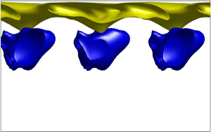
The optimal perturbations are visualised in this paper as isosurfaces of maximum and minimum streamwise velocity perturbations  $u_1$, e.g. as in figure 3 shown for linear optimal perturbations. In this figure and those to follow, a yellow isosurface is plotted at a certain percentage of the maximum over the channel of that quantity at that time, while a blue isosurface indicates regions where the quantity is at the same percentage of the minimum (a negative quantity).

Figure 3. Three-dimensional linear optimal perturbation ( $E_0=10^{-8}$), which maximises the cost functional in (2.13) for (a) unstratified ( $\Delta T=0$) and (b) stratified ( $\Delta T=40\ \textrm {K}$) channel flow for $Re=500$, $\mathcal {T}=4$ and $Pr=7$. The mean flow is along the positive $x$ as marked by arrows in (a,b). The colours are the $40\,\%$ isosurfaces of the maximum (yellow) and minimum (blue) values of the streamwise perturbations $u_1$. The isosurfaces for other stratification levels ( $\Delta T = 20\ \textrm {K}$ and $60\ \textrm {K}$) are qualitatively similar to (b), with $40\,\%$ isosurfaces of $u_1$ localised near the hot wall, where viscosity is lower.
The linear optimal perturbation ( $E_0=10^{-8}$) consists of an array of streamwise velocity perturbations inclined against the mean flow and shear, on both sides of the channel for the unstratified case (figure 3a). In the stratified case, similar structures are seen, but all perturbations are remarkably localised close to the hot wall, where the viscosity decreases towards the wall, with practically no action on the cold wall (figure 3b). Such localisation of linear optimal perturbations was also found by Jose, Brandt & Govindarajan (Reference Jose, Brandt and Govindarajan2020) using SVD studies on a channel with viscosity stratification and weak gravity. For our chosen target time of $\mathcal {T}=4$, we find that the non-modal energy growth and the shapes of the optimal perturbations are similar whether we optimise for a cost functional with energy growth at the target time or with time-integrated energy as in (2.13). As mentioned, the linear optimal perturbation for maximising energy at a target time can also be obtained by an SVD of the respective Orr–Sommerfeld and Squire operators for the unstratified (Schmid et al. Reference Schmid, Henningson and Jankowski2002) and viscosity-stratified (Chikkadi, Sameen & Govindarajan Reference Chikkadi, Sameen and Govindarajan2005) cases. The streamwise and spanwise wavenumbers of the linear optimal perturbation from SVD for $\mathcal {T}=4$ and $Re= 500$ are $k_x\approx 2$ and $k_z\approx 4$, respectively, for an unstratified channel and $k_x\approx 2$ and $k_z\approx 5$, respectively, for the viscosity-stratified channel with $\Delta T= 40\ \textrm {K}$. Quantised for channel length, we observe from figure 3 that these wavenumbers can be seen in the linear optimal perturbations obtained from direct-adjoint looping with $E_0=10^{-8}$. The periodic boundary conditions in the streamwise and spanwise directions restrict the wavenumbers to be zero or such that the channel dimension is an integer multiple of the corresponding wavelength. Besides revealing the localisation of the arrays of vortices near the hot wall due to viscosity stratification, this result is also a validation for our direct-adjoint looping.
The corresponding root mean square (r.m.s.) profiles of velocity perturbations of the linear optimal perturbations are shown in figure 4, where the quantities have been averaged in the streamwise and spanwise directions. There is a significant proportion of initial amplitude in each velocity component, and stratification increases the proportion of energy in the spanwise and wall-normal perturbations  $u_3$ and $u_2$ in relation to the streamwise perturbations. In $u_2$, the difference between stratified and unstratified cases is larger than the difference between different levels of stratification. The localisation of all perturbations on the hot side of the channel is underlined in this figure.

Figure 4. Wall-normal profiles of root mean square (r.m.s., spatially averaged in the  $x$ and $z$ directions) of the linear optimal perturbations ( $E_0 = 10^{-8}$). (a) Streamwise velocity perturbations $u_1$, (b) wall-normal velocity perturbations $u_2$ and (c) spanwise velocity perturbations $u_3$ for various wall-temperature differences $\Delta T$ (in K). The solid and the dash-dotted lines in (a) correspond to the isosurfaces shown in figures 3(a) and 3(b), respectively.
The time evolution, obtained by solving the direct equations initialised with the linear optimal perturbation, suggests the reason for its shape. For both the unstratified and stratified cases, shown in figures 5 and 6, respectively, velocity perturbations are initially tilted against the mean shear, and as time progresses, lean into the shear as they stretch. This is the well known, and probably oldest to be described, linear growth mechanism, the Orr mechanism (Orr Reference Orr1907), where the tilting and the subsequent energy growth is driven by the base, or laminar, shear. In stratified laminar flow, the magnitude of shear is larger near the less-viscous wall, which for liquids is the hot wall (figure 2b). So, the Orr mechanism is much more efficient near the hot wall. It follows that, for a given  $E_0$, better growth can be achieved by placing perturbations in the high gradient region, which explains the localisation of the initial velocity perturbations in stratified flow (figures 3b and 4). The evolution of the optimal perturbations results in algebraic energy growth of disturbances for short durations of time, which eventually decays as shown in figure 7. As can be seen, the maximum algebraic growth need not be at the target time. For the linear optimal perturbations, the energy growth for stratified flow is larger than for unstratified flow, but this conclusion will not be the same for the nonlinear optimal perturbations, as we shall see.

Figure 5. Evolution of the linear unstratified optimal perturbation shown at two angles, at times (a,b)  $t=0$, (c,d) $t=2$, (e,f) $t=\mathcal {T}=4$, (g,h) $t=6$ and (i,j) $t=8$. The structures are initially aligned against the shear, and as time progresses, realign along the shear. Refer to supplementary movie 1 available at https://doi.org/10.1017/jfm.2020.1160 for the full evolution.

Figure 6. Evolution of the linear viscosity-stratified optimal perturbation ( $\Delta T = 40\ \textrm {K}$) shown at two angles. Optimal perturbations are strongly localised on the top (hot) wall unlike in figure 5, and the Orr mechanism is in evidence. The times are as in figure 5. Refer to supplementary movie 2 for the full evolution.

Figure 7. Energy growth with time of the linear optimal perturbations ( $E_0 = 10^{-8}$) for various stratification strengths. The target time of optimisation for all of them is $\mathcal {T} = 4$. The labels at $t=2,4,6,8$ on the solid line correspond to labels in figure 5.
We thus find that the Orr mechanism is the dominant linear growth mechanism for small energy levels in this short target time window. We note that, for longer target times, the dominant mechanism may be different. This mechanism has also been observed in the time evolution of (nonlinear) minimal seeds by Duguet et al. (Reference Duguet, Monokrousos, Brandt and Henningson2013) in plane Couette flow during intermediate times before eventually reaching a turbulent state. The other well-known linear growth mechanism, the lift-up mechanism (Landahl Reference Landahl1980; Brandt Reference Brandt2014), is not observed in the evolution of the linear optimal perturbation at small  $E_0$. Before we study nonlinear optimal perturbations, it is instructive to study what would happen if the linear optimal perturbation were of large enough amplitude to trigger nonlinearities. To this end, we rescale the initial energy of the linear optimal perturbations (calculated with $E_0=10^{-8}$) to a higher initial energy, $E_0=10^{-2}$, while maintaining the shape of the initial conditions corresponding to the case shown in figure 3(b) for $\Delta T = 40\ \textrm {K}$. The full nonlinear evolution of the streamwise velocity perturbations for this case is shown in figure 8. The low momentum fluid is transferred away from the walls, displaying features of the classical lift-up mechanism driven by streamwise vortices (not shown). Negative perturbation velocities (in blue) are seen in the channel interior as opposed to positive perturbation velocities (in yellow) at the top wall. However, given that the mean velocity is higher towards the interior of the channel away from the walls, these negative perturbation structures could move faster than the positive perturbation structures in terms of total speed. Comparing figures 6 and 8, we see that the nonlinear evolution of the (scaled-up) linear optimal perturbation is very different from the linear evolution of the linear optimal perturbation. The nonlinear evolution of the linear optimal perturbation for the unstratified case (not shown) also shows a lift-up-type mechanism in operation, albeit at both walls, and is symmetric around $y=0$. The physical mechanism for energy growth at small energy levels ( $E_0 = 10^{-8}$) is thus the Orr mechanism and that at high energy levels ( $E_0 = 10^{-2}$) is indicative of the lift-up mechanism. As we discuss below, in particular for stratified flow, the linear optimal perturbations are not the most efficient structures to extract energy from the mean flow into the perturbations for higher energy levels.

Figure 8. The linear viscosity-stratified optimal perturbation ( $\Delta T = 40\ \textrm {K}$) calculated with $E_0 = 10^{-8}$ and scaled to nonlinear initial energy $E_0 = 10^{-2}$ is evolved by the fully nonlinear direct equations. Two different angles are shown, showing that the lift-up mechanism is in evidence. The times are as in figure 5. Refer to supplementary movie 3 for the full evolution. For the corresponding streamwise vorticity evolution, refer to figure 1 in the supplementary material.
3.2. The nonlinear optimal perturbation and its evolution
The perturbation leading to the maximum energy growth for the highest  $E_0$ of $10^{-2}$ considered here is referred to as the nonlinear optimal perturbation. Isosurfaces of the nonlinear optimal streamwise velocity perturbation (figure 9) and streamwise–spanwise averaged r.m.s. wall-normal nonlinear optimal velocity profiles (figure 10) show some localisation towards the hot wall due to viscosity stratification. But remarkably, unlike in the linear case (figures 3 and 4), there is significant perturbation energy on both walls of the channel for the stratified nonlinear optimal perturbation. Figure 10, in stark contrast to figure 4, makes it clear that the asymmetry between the two sides of the channel is small for the nonlinear optimal perturbation, whereas for the linear optimal perturbation, energetic structures were absent in the bottom half of the channel. But in the nonlinear optimal perturbation too, the asymmetry increases with increasing stratification, with more structures at the hot wall. The streamwise velocity perturbations are now arranged in a series of elongated (mainly in the flow direction, but with a spanwise inclination) high and low momentum zones near the walls. Increasing the stratification level makes the population near the cold wall smaller (but not insignificant). From figure 10 we observe a significant contribution to the initial perturbation kinetic energy from all three components of velocity.

Figure 9. The  $40\,\%$ isosurfaces of the maximum (yellow) and minimum (blue) values of the streamwise perturbations $u_1$ of the nonlinear optimal perturbation ( $E_0 = 10^{-2}$) with (a) $\Delta T = 0$ (unstratified); and of the viscosity-stratified nonlinear optimal perturbation with (b) $\Delta T = 20\ \textrm {K}$ and (c) $\Delta T = 40\ \textrm {K}$. (d) The $20\,\%$ isosurfaces of the maximum (yellow) and minimum (blue) $u_1$ for the viscosity-stratified nonlinear optimal perturbation with $\Delta T = 60\ \textrm {K}$. A slightly lower isosurface value had to be shown in (d) for better visualisation.

Figure 10. Wall-normal profiles of (a) streamwise velocity fluctuations  $u_1$, (b) wall-normal velocity fluctuations $u_2$ and (c) spanwise velocity fluctuations $u_3$, averaged across the $x$ and $z$ coordinates, of the nonlinear optimal perturbations ( $E_0 = 10^{-2}$) for various stratification strengths.
The energy–time graphs corresponding to the evolution of the nonlinear optimal perturbations in figures 9 and 10 are shown in figure 11 for various stratification levels. Figure 11(a) shows the cost functional  $\mathcal {J}_{opt}(\mathcal {T})$ of the optimal perturbation, which is the quantity that we optimised for, while figure 11(b) shows the volume-averaged kinetic energy as a function of time. Growth is algebraic in the nonlinear regime as well, and perturbations decay soon after the target time of optimisation. Unlike in the linear evolution of the linear optimal perturbation, there is no qualitative difference between the levels of growth in the unstratified case and those at various levels of stratification. Whether this will hold true over longer target times will need investigation. We are now in a position to compare the evolution, by the modified Navier–Stokes equation, of the linear and the nonlinear optimal perturbations, both starting from the same initial energy of $E_0=10^{-2}$, in figure 12. We may first satisfy ourselves of the higher energy growth in the evolution of the nonlinear optimal perturbation as compared to the linear optimal perturbation, consistent with the definition of the nonlinear optimal perturbation. For the unstratified flow, for a short target time, it turns out that the linear and nonlinear optimal perturbations show similar growth, although the linear is of course lower, whereas the linear optimal perturbation shows a much lower growth in the stratified flow than the nonlinear optimal perturbation (comparing the dashed black line to the dashed red one in figure 12). This is consistent with the cold wall becoming more prominent in the evolution of the nonlinear optimal perturbation, as we shall discuss below. It is also worth mentioning that, on comparison with figure 7, we see that the growth of energy of the linear optimal perturbation, as a ratio of the initial energy, is significantly lower with nonlinear evolution, for initial conditions differing only in amplitude. However, the absolute value of perturbation energy always remains larger than the linear case since the initial perturbation was large. When the initial perturbation is large, the available energy from the laminar flow becomes a limiting factor, which could result in the lower growth, as a ratio.

Figure 11. Time evolution of (a) the cost functional  $\mathcal {J}_{opt}(t)$ as in (2.14) and of (b) energy, of the nonlinear optimal perturbations for various stratification strengths. The time of optimisation is $\mathcal {T}=4$ for all.

Figure 12. Evolution of energy of the linear and nonlinear optimal perturbations when evolved with the modified Navier–Stokes equation with  $E_0=10^{-2}$. Solid lines are for the unstratified cases ( $\Delta T = 0$) while the dotted lines are for stratified cases with $\Delta T = 40\ \textrm {K}$. Other stratification levels (not shown) show similar behaviour to $\Delta T = 40\ \textrm {K}$.
We now discuss how stratification changes the mechanism of subcritical disturbance growth and how nonlinear optimal perturbations are fundamentally different from linear optimal perturbations in this regard. Initially proposed by Hamilton, Kim & Waleffe (Reference Hamilton, Kim and Waleffe1995) and Waleffe (Reference Waleffe1997) and summarised by Brandt (Reference Brandt2014), the regeneration/self-sustaining cycle of wall turbulence involves three steps, (i) lift-up, i.e. transportation of low (high) momentum fluid away from (towards) the wall by streamwise vortices, to form streamwise independent streaks of low (high) momentum away from (near) the wall, (ii) break down of these by inflectional secondary instability to acquire streamwise dependence and (iii) regeneration of elongated vortices by nonlinear interactions between oblique modes. These arguments were initially made with the linear optimal perturbation in mind. Through a direct-adjoint looping optimisation methodology, Cherubini et al. (Reference Cherubini, De Palma, Robinet and Bottaro2011) for a boundary layer and Cherubini & De Palma (Reference Cherubini and De Palma2013) for a Couette flow showed that it is much more efficient for the lift-up to be driven by streamwise-modulated vortices in the first place. The nonlinear optimal perturbation inherently contains such streamwise modulation. This is referred to as the modified lift-up mechanism, as it can bypass the stage of secondary (streak) instability en route to transition to turbulence.We detect similar optimal perturbation structures here for a channel flow, both in the unstratified and stratified cases. Their evolution in time by the modified Navier–Stokes equations is shown in figure 13 for the unstratified case. A modified lift-up mechanism similar to Cherubini et al. (Reference Cherubini, De Palma, Robinet and Bottaro2011) and Cherubini & De Palma (Reference Cherubini and De Palma2013) is seen to be in operation, where low momentum fluid is lifted off the wall and high momentum fluid is brought closer to the wall by streamwise-modulated vortices (vortices not shown). This translates into the algebraic growth of perturbation kinetic energy seen in figure 11.

Figure 13. Evolution of the nonlinear unstratified optimal perturbation with  $E_0=10^{-2}$, shown at two angles. The times are as in figure 5. Refer to supplementary movie 4 for the full evolution. For the corresponding streamwise vorticity evolution, refer to figure 2 in the supplementary material.
The evolution of the nonlinear optimal perturbation in stratified flow is shown in figure 14. As mentioned earlier, the inception of an inflection point due to lift-up may be expected to be more efficient near the less-viscous wall as the wall-normal velocity gradient is larger, and lift-up is usually associated with  $u_2 \partial {U}/\partial {y}$ (Cherubini et al. Reference Cherubini, De Palma, Robinet and Bottaro2011). Consistent with this, we have a larger population of optimal perturbation structures near the less-viscous wall, as seen in figure 9(a,b). Since mean shear is smaller at the cold wall, its lift-up capability is lower, and therefore it may be argued that structures which are already a little away from the cold wall can grow better on the cold side. This is borne out by the optimal perturbation structures seen in the bottom half of figure 14(b). An interesting feature of the evolution of the viscosity-stratified nonlinear optimal perturbation, which distinguishes it from the unstratified case as well as from the evolution of the linear optimal perturbation, is that as time progresses action at the cold wall is increasingly significant, and the high-speed structures at the hot wall shrink in wall-normal extent. The evolution of perturbations at the cold wall is strong enough to create points of inflection in the $x\text {--}z$-averaged velocity profiles, and this will be discussed with the aid of figure 15. We shall refer to a ‘strengthening (weakening)’ of inflectional profiles when the profile becomes more (less) strongly wavy in the wall-normal direction. In panel (a) of this figure, we see that the unstratified flow progresses steadily towards inflection, maintains this up to approximately $t=10$ and become less inflectional thereafter. The profiles are symmetric. In fact, the perturbations in all cases decay at long times, given low Reynolds number and small target time of optimisation employed here. In figure 15(b) the evolution of the profile in the stratified case is shown. There is a strengthening of the inflectional profile at early times at both walls, with the hot wall being more inflectional. After approximately $t=4$, the profile becomes weaker near the hot wall and more strongly inflectional than before on the cold side, before eventually weakening at long times. The corresponding profiles of the $x\text {--}z$-averaged total viscosity are shown in figure 15(c). Upon comparing with the laminar viscosity profile, up to a time of approximately $10$, on the colder side, we see that higher-viscosity fluid from the cold wall has been lifted up towards the centreline and lower-viscosity fluid from the central portion of the channel has been carried towards the wall. A similar exchange is visible on the hot side of the channel as well, but with opposite signs of viscosity change. At the long time of $t=16$, we see a mixing of fluids. Below, we address the question: If lift-up is more efficient at the less-viscous wall, why do perturbations grow near the other wall?

Figure 14. Evolution of the nonlinear viscosity-stratified optimal perturbation ( $\Delta T = 40\ \textrm {K}$) with $E_0=10^{-2}$, shown at two angles. The times are as in figure 5. Refer to supplementary movie 5 for the full evolution. For the corresponding streamwise vorticity evolution, refer to figure 3 in the supplementary material.

Figure 15. The total streamwise velocity at various times averaged across the  $x$ and $z$ coordinates for (a) the nonlinear unstratified optimal perturbation and (b) the nonlinear viscosity-stratified optimal perturbation for $\Delta T=40\ \textrm {K}$. (c) The evolution of the total viscosity profile for the flow corresponding to (b). Solid black lines in each for $t=0$, solid red for $t=2$, solid blue for $t=4$, dashed black for $t=6$, dashed red for $t=8$, dashed blue for $t=10$ and solid green for $t=16$.
After the inception of lift-up, near the hotter wall, less-viscous fluid of low momentum is brought away from the wall to the vicinity of more-viscous and high momentum fluid, and the opposite happens on the colder wall. Thus the low (high) momentum streaks near the hotter wall are composed of less (more) viscous fluid, but those near the colder wall are composed of more (less) viscous fluid than the local laminar values. This is evident from the conditionally averaged viscosity profiles in figures 16(a) and 17(a) at times  $t=2$ and $6$, respectively. Here, at each $y$ location, the viscosity $\langle {\mu _+}\rangle$ is averaged over all positive $u_1$ cells over the $x\text {--}z$ plane, and $\langle {\mu _-}\rangle$ is the viscosity averaged over negative $u_1$ cells in the same plane. A small cutoff $\epsilon =0.001$ in the velocity has been used for this averaging, and it has been checked that the profiles are insensitive to the exact choice of $\epsilon$. These plots establish that, on the colder side of the channel, low-speed regions are correlated with reduced viscosity, and high-speed regions correlate with elevated viscosity, with the opposite correlations on the hotter side. The instantaneous streamwise velocity perturbations in four different $x\text {--}z$ planes are shown in figures 16 and 17 in panels (b–e). The spanwise widths and spacing of the low- and high-speed streaks are significantly larger on the cold side than on the hot side. Secondly, the streaks persist up to $t=6$ on the cold side, whereas on the hot side the structure is practically lost by this time. A physical argument for the relative persistence near the colder wall is as follows. Consider that the streamwise pressure gradient is similar across the span of the channel. High-speed streaks of low viscosity alternating with the low-speed flow of higher viscosity would be maintained by this pressure gradient. On the other side, i.e. at the hot wall, a higher-viscosity fluid of higher forward speed would tend to slow down, and a higher-viscosity fluid of lower speed to speed up, in response to a similar streamwise pressure gradient. The greater persistence of streaks on the colder side is thus a consequence of the basic asymmetry in the mechanics of the lift up on the two sides.

Figure 16. Flow driven by the nonlinear viscosity-stratified optimal perturbation at  $\Delta T = 40\ \textrm {K}$ and time $t=2$. (a) Viscosity profiles averaged across the $x$ and $z$ coordinates for positive streamwise velocity perturbation $u_1 > \epsilon$ in red, and for $u_1 < -\epsilon$ in blue. The laminar viscosity profile is shown as a dashed black line. The four vertical black dotted lines with labels denote the $y$ locations of the plots in (b–e). Instantaneous streamwise velocity perturbations $u_1$ are shown in the $x\text {--}z$ plane at $y$ locations (b) $-0.25$, (c) 0.25, (d) $-0.75$ and (e) 0.75. Refer to figure 14(c) for a three-dimensional view of isosurfaces of $u_1$ at this time and the red solid line in figure 15(b) for the total $U(\kern-0.004em y)$ averaged in $x$ and $z$ at this time.


In figure 9(c) we had seen that the spanwise variation of the velocity perturbations had different apparent wavenumbers on the two walls. The slices in figures 16 and 17 clarify this to be a sinuous variation. Such variation is known to be responsible for the ultimate breakdown of streaks (Waleffe Reference Waleffe2009). A study at higher Reynolds number and longer target time could reveal this. Besides, the inflectional instability, discussed below for the stratified case, extracts energy from the streaks (Waleffe Reference Waleffe2009) allowing further energy growth beyond the lift-up. Further studies at higher Reynolds numbers and longer target times will be needed to explore these mechanisms in viscosity-stratified flows.
The observations in figures 15–17 enable us to schematically illustrate the lift-up process in stratified flow, in figure 18. Ellingsen & Palm (Reference Ellingsen and Palm1975) described the creation of inflectional profiles due to the redistribution of velocity by streamwise independent, but three-dimensional, velocity perturbations, i.e. due to the lift-up effect. The nonlinear mechanism in the evolution of the optimal structures is the modified lift-up (Cherubini et al. Reference Cherubini, De Palma, Robinet and Bottaro2011; Cherubini & De Palma Reference Cherubini and De Palma2013). In figure 18, we highlight the effect of viscosity stratification on the lift-up mechanism alone. Panel (a) shows stronger inception of inflection near the hot wall at early times, which is caused by the rolls being concentrated near that wall. On the left of panel (b) we sketch how this lift-up results in the exchange of viscosities. On the right of this panel, we see how this exchange of viscosities results in the strengthening of the inflectional profile on the cold wall and weakening on the hot wall. Wherever viscosity is higher than the surrounding laminar flow, gradients are lowered, and wherever it is lower, gradients are relatively increased. Thus, the low-viscosity streak at the cold wall brings with it higher velocity gradients, leading to stronger lift-up. The nonlinear optimal of figure 9 has a non-zero velocity perturbation near the colder wall, unlike the linear optimal of figure 6. This is because streaks persisting for longer at the cold wall contribute to nonlinear energy growth. The persistence of high momentum and low-viscosity streaks, combined with stronger inflection in the velocity profile near the colder wall, is consistent with the observations of previous DNS studies (Zonta et al. Reference Zonta, Marchioli and Soldati2012; Lee et al. Reference Lee, Jung, Sung and Zaki2013) concerned with turbulence in stratified flow. In boundary layer flow (Lee et al. Reference Lee, Jung, Sung and Zaki2013) heating the flat plate and hence making fluid less viscous in the vicinity leads to suppression of turbulence and for channel flow (Zonta et al. Reference Zonta, Marchioli and Soldati2012) turbulence is suppressed on the hot/less-viscous wall and enhanced on the cold/more-viscous wall. Cherubini et al. (Reference Cherubini, De Palma, Robinet and Bottaro2011) and Cherubini & De Palma (Reference Cherubini and De Palma2013) highlight the importance of the Orr and lift-up mechanisms, both linear mechanisms, in the creation of subcritical transition through minimal seeds of turbulence transition (obtained by optimising over much larger target times as compared to what we study in this paper). Duguet et al. (Reference Duguet, Monokrousos, Brandt and Henningson2013) also identify the existence and importance of these mechanisms in the time evolution of minimal seeds in Couette flow, and the subsequent breakdown of the streaks to instabilities. Recently, Vavaliaris, Beneitez & Henningson (Reference Vavaliaris, Beneitez and Henningson2020) also reported the dominance of these mechanisms in the initial stages of subcritical turbulence in a boundary layer. We have shown how viscosity stratification in a channel acts to modify these mechanisms. For the short target time ( $\mathcal {T}=4$) optimal perturbations at the relatively small Reynolds number ( $Re=500$) that we have studied, the interaction required for nonlinear regeneration of the streaks and hence completing the regeneration cycle en route to transition (Waleffe Reference Waleffe2009) is absent. But the primary role of viscosity stratification in the initial stages of the nonlinear non-modal process has been revealed.

Figure 18. Schematic of the lift-up mechanism influenced by viscosity stratification: (a) inception of the inflection in the velocity profile is stronger near the less-viscous wall as it has larger wall-normal velocity gradient, (b) persistence of the inflection created is greater near the cold/more-viscous wall because the streak  $C2$ of high momentum can sustain higher wall-normal gradients of velocity than before, whereas the streak of low momentum, $C3$, which has higher viscosity velocity gradients within it, will be lowered. The opposite happens on the other wall, where high momentum fluid $H2$ has higher-viscosity and low momentum fluid $H3$ has lower viscosity than the local laminar value. The dashed line represents the undisturbed laminar profile, the dash-dotted line and the solid lines are representations of early and later times, respectively.
3.3. Effect of Prandtl number
We performed simulations at three Prandtl numbers:  $Pr=0.1, 7$ and $5000$, for $\Delta T=20\ \textrm {K}$. Our lowest Péclet number, i.e. the product of the Reynolds and the Prandtl numbers, is $50$, which is too large for diffusion of the temperature perturbations to qualitatively change the behaviour over our simulation times. We confirm this in our simulations. Slices of temperature and viscosity perturbations are shown in figure 19 for two values of $Pr$, when evolved with the corresponding nonlinear optimal perturbation up to the target time. We see that diffusion effects are greater at the lower Prandtl number, so viscosity variations persist better at the higher $Pr$, while we find very similar structures and their evolution (not shown) at all Prandtl numbers. However, in studies over longer target times, of the process of transition to turbulence, we expect the Prandtl number to play an important role.

Figure 19. Temperature perturbations at target time at  $z = {\rm \pi}/2$ for (a) $Pr=0.1$ and (c) $Pr=7$ when started with the corresponding nonlinear viscosity-stratified optimal perturbation ( $\Delta T = 20\ \textrm {K}$). The corresponding viscosity contours at same time are in (b,d). Note the presence of higher gradients in temperature and viscosity in (c,d), respectively. The colour bars in (a,c) are different.
4. Conclusions
In this study we have derived, for the first time to our knowledge, the adjoint modified Navier–Stokes equations for a viscosity-stratified flow. We have developed a numerical solver for the direct and adjoint equations in an iterative loop in three dimensions, to find optimal initial conditions in the linear limit as well as for a finite initial perturbation energy. We have shown that viscosity stratification brings important modifications to the operation of the lift-up mechanism in the early stages of disturbance growth. For the optimisation time considered here, initially stronger lift-up is set up at the hot (less-viscous) wall due to the higher mean velocity gradient, but the lift-up at the cold (more-viscous) wall increases in strength later, while that at the hotter wall weakens. Significantly, at the colder wall, high-speed streaks are more persistent, of larger spanwise extent, and give rise to a strengthening of the inflectional profile. We have presented physical arguments for these observations based on the viscosity of the fluid in the high- and low-speed streaks undergoing the lift-up. Thus the action shifts from the hotter wall to the colder wall as time progresses. Most of the features we observe in the evolution of the nonlinear optimal perturbation are completely missed in the linear study. A linear optimal perturbation of small amplitude will only display the Orr mechanism and not the lift-up. At higher amplitudes, lift-up will be seen, but only at the hot wall. In fact, no perturbations are ever seen near the cold wall with the linear optimal perturbation.
This work suggests several directions for future research. This study has been for a short target time, so a starting point for understanding the role of viscosity stratification in the transition to turbulence will be the study of nonlinear optimal perturbations over long target times. The question of the minimal seed for triggering turbulence could be of importance in this context. With an increase in the target time and Reynolds number, the existence and the interplay of the observed Orr and the modified lift-up mechanisms could be investigated. Vermach & Caulfield (Reference Vermach and Caulfield2018) made an interesting finding that the initial condition which produces the most efficient mixing could be quite different from that which gives the highest energy growth. Recognising that most flows where questions about mixing are relevant are also stratified in viscosity indicates this as an area of study. We expect the effect of Prandtl number to be pronounced in flows with a sharp stratification, e.g. the flow of miscible fluids of different viscosity, and also at long times in continuously stratified flows, and this bears investigation. We have neglected gravity in this study but most flows with a composition or temperature variation are subject to buoyancy effects. This combination will make for an interesting study. Finally, given the number of industrial applications for which viscosity stratification is important, a variety of experimental studies are called for. We hope that this first work on the effects of viscosity stratification in nonlinear optimal perturbation growth will give impetus to such studies.
Supplementary material and movies
Supplementary material and movies are available at https://doi.org/10.1017/jfm.2020.1160.
Acknowledgements
G. K. Batchelor, and stories about him, have been an inspiration to us over the years, and it is a pleasure to dedicate this paper to his memory. The authors thank three anonymous referees for their critical feedback which has helped sharpen many aspects of this paper. The authors would like to thank S. Jose and V. Vasan for helpful discussions during the development of the solver and on non-modal analysis. R.T. and R.G. acknowledge support, under project no. 12-R&D-TFR-5.10-1100 of the Department of Atomic Energy and the Ocean Mixing and Monsoon program of the Ministry of Earth Sciences, of the Government of India. Simulations were performed in the high-performance computing facility of ICTS, Bengaluru.
Declaration of interests
The authors report no conflict of interest.
Appendix A. More on the numerical method and its validation
The  $x$ and $z$ directions in figure 1 are the homogeneous directions and we define periodic boundary conditions in these, except in the pressure. We impose no-slip boundary conditions at the walls at $y={\pm }L_y$. For all the analyses, we use a non-dimensional size of $L_x = 2{\rm \pi}$, $L_y = 2$, and $L_z = {\rm \pi}$ in which the streamwise extent is smaller than in Vermach & Caulfield (Reference Vermach and Caulfield2018), while the spanwise extent is the same. Our channel size is the same as in the two-dimensional study of Foures et al. (Reference Foures, Caulfield and Schmid2013).
A.1. Grid and numerical method
The gradients in the velocity and temperature fields are higher with nonlinear initial energy ( $E_0 = 10^{-2}$) when compared to linear initial energy ( $E_0 = 10^{-8}$). In $x$,
$x$,  $y$ and $z$, we use $100 \times 209 \times 50$ grid points for $E_0 = 10^{-2}$, while we use $50 \times 209 \times 25$ grid points for $E_0 = 10^{-8}$. The makes the grid spacing in the $x$ and $z$ directions equal, at 0.06 for $E_0 = 10^{-2}$ and at 0.12 for $E_0 = 10^{-8}$. For a nonlinear stratified case with $\Delta T = 20$ and $E_0 = 10^{-2}$, the maximum difference between $E(\mathcal {T}) = \langle \langle \boldsymbol {u}(\boldsymbol {x},t)\boldsymbol {\cdot }\boldsymbol {u}(\boldsymbol {x},t)\rangle \rangle /2$ with a grid of $100\times 209 \times 50$ and a finer grid of $128\times 209 \times 64$ (this produces grid spacing the same as that of Vermach & Caulfield Reference Vermach and Caulfield2018) is $O(10^{-5})$.
The wall-normal or the  $y$ direction is discretised into a staggered combination of base and fractional grids (e.g. see Bewley Reference Bewley2012). This puts a fractional grid point at the mid-location of two base grid points. The streamwise and spanwise velocities, pressure and temperature are defined on the fractional grid and the wall-normal velocity on the base grid. A hyperbolic tangent function
 \begin{equation} y_j = \tanh\left( k \left[ \frac{2(j-1)}{N_Y} - 1 \right] \right), \quad j=1,2, \ldots N_Y, \end{equation}
where  $N_Y$ is the number of grids in the wall-normal direction, is used to cluster both the fractional and the base grid points towards the walls. The value of $k$ in (A1) has been kept constant at 1.5 and it creates a $y$-grid with $\Delta y_{max}$ = 0.0159 (near the centre of the channel) and $\Delta y_{min}$ = 0.0029 (near both the walls). The wall-normal spatial derivatives are computed using second-order central finite difference method. The spatial derivatives in $x$ and $z$ are calculated using fast-Fourier transform and we truncate the Fourier series using the 2/3-rule to prevent aliasing (e.g. see Canuto et al. Reference Canuto, Hussaini, Quarteroni and Zang2007). We employ a time-stepping algorithm which is a combination of an explicit method (Runge–Kutta–Wray) for the nonlinear (convective) terms and an implicit method (Crank–Nicolson) for the linear (viscous) terms and the wall-normal derivatives.
A.2. Convergence to the optimal
To converge to the optimal perturbation, we start with a guess of the same at the outset of the very first direct-adjoint loop. After we have completed one iteration by going forward and backward with the direct and adjoint equations, we need to update the guess for the next iteration. We employ the update-by-rotation technique of Foures et al. (Reference Foures, Caulfield and Schmid2013) which involves a line search after the adjoint leg of the direct-adjoint loop is completed. This first amounts to updating the direct variables at  $t=0$ after the $n$th iteration by an angle $\zeta$, between $0^\circ$ and $360^\circ$, as
 \begin{equation} u_i^{n+1}=u_i^{n}\cos{\zeta}+f_i(\boldsymbol{u}^{n},\boldsymbol{v}^{n})\sin{\zeta}, \end{equation}
where the exact functional form of  $f_i$ in terms of the direct velocities $\boldsymbol {u}^{n}$ and adjoint velocities $\boldsymbol {v}^{n}$ is provided in Foures et al. (Reference Foures, Caulfield and Schmid2013). The next step involves evolving the direct equations with $u_{i}^{n+1}$ for each update angle $\zeta$ and noting the cost functional. The update angle that provides the largest cost functional is chosen as our desired update angle $\zeta _{max}$. The iteration continues with the updated guess $u_i^{n+1}=u_i^{n}\cos {\zeta _{max}}+f_i(\boldsymbol {u}^{n},\boldsymbol {v}^{n})\sin {\zeta _{max}}$. We have tried various step sizes for the angle search and, after a few iterations, found the direct-adjoint loop to ultimately converge to a zero angle, i.e. where the direct variables from the previous iteration are the optimal perturbations ( $u_i^{n+1}=u_i^{n}$) within the tolerance of the step size. As expected, the number of iterations required to converge to zero angle is inversely proportional to the angle step size. As mentioned in § 2.3, at this point, we find the residual as defined in other studies (Vermach & Caulfield Reference Vermach and Caulfield2018) to be of $O(10^{-3}\text {--}10^{-4})$. For the geometry considered in this paper, the direct-adjoint loop optimises for $O(10^6)$ variables for the nonlinear case, and as stated by Vermach & Caulfield (Reference Vermach and Caulfield2018), it would be instructive to regard the corresponding optimal perturbations as approximations. It takes $O(100)$ iterations to converge to the nonlinear optimal perturbation, with $E_0 = 10^{-2}$, for the unstratified as well as the stratified cases, similar to the number in Vermach & Caulfield (Reference Vermach and Caulfield2018), while it takes less than 50 iterations to converge to the linear optimal perturbation ( $E_0 = 10^{-8}$, both unstratified and stratified) when starting from random initial conditions. Imposing an optimal perturbation of a similar parameter set as our initial guess allows much faster convergence to the same optimal perturbation as before, akin to method of continuation. The ease of convergence to the linear optimal perturbation has also been reported in the studies cited in the text. It is seen that with an increase in the strength of viscosity stratification, the structure of the nonlinear optimal perturbations become noisier, and perfect isosurfaces of streamwise perturbation velocity are harder to obtain.
Only for the validation purpose with Vermach & Caulfield (Reference Vermach and Caulfield2018), we use a longer channel with  $L_x=4{\rm \pi}$. With our direct-adjoint looping solver, for target time $\mathcal {T}=2$, we achieve a $G(\mathcal {T})$ of over $93\,\%$ of that obtained by Vermach & Caulfield (Reference Vermach and Caulfield2018) at the target time, which incidentally is the only existing study to our knowledge on nonlinear optimal perturbation in unstratified three-dimensional channel flow. The isosurfaces of the streamwise velocity that we obtain for the nonlinear optimal perturbation with $E_0=10^{-2}$, starting from random initial conditions, closely agree with those of Vermach & Caulfield (Reference Vermach and Caulfield2018). In particular, both computations result in optimal perturbations which are elongated in the streamwise direction, with streamwise wavelength far larger than can be accommodated in the channel of $4{\rm \pi}$ length, spanwise wavenumber of $k_z=6$, and very similar levels of obliqueness. A more perfect numerical agreement is not to be expected as these optimal perturbations are known to be numerically delicate (Foures et al. Reference Foures, Caulfield and Schmid2013) and might vary with varying resolution of the optimiser. Nonlinearity makes the problem one of non-convex optimisation and it is not clear how to arrive at the global maximum, or how the existence of more than one local maximum can be resolved (Kerswell Reference Kerswell2018). A close examination of the two structures shows that there are small differences in the symmetry of arrangement, so we might have arrived at a closely resembling but different optimal, as compared to Vermach & Caulfield (Reference Vermach and Caulfield2018). A check we performed to make sure we have converged to a local optimum is to start from different initial conditions of random noise of the desired amplitude, as well as an optimal perturbation from a different parameter set, to ensure that the optimal perturbations we arrive at are the same within the finite difference errors ( $O(10^{-4})$). For the viscosity-stratified case, we ran the direct-adjoint loop at very low initial energy of $E_0=10^{-8}$ to get the linear optimal perturbation by maximising $E(\mathcal {T}) = ({\|\boldsymbol {u}(\boldsymbol {x}, \mathcal {T})\|_{\mathcal {V}}^{2}})/2$, compared it to the linear viscosity-stratified optimal perturbation obtained from SVD, and obtained excellent agreement as already mentioned in § 3.1.


