


NOMENCLATURE
- Ak
influenced coefficient of doublet
- Bk
influenced coefficient of source
- C up
pressure coefficient of upper rotor
- C lp
pressure coefficient of lower rotor
- n
outward unit normal vector
- N
number of panels of blade surface
- N w
number of panels of wake surface
- p
local pressure [Pa]
- p u
local pressure of upper rotor [Pa]
- p l
local pressure of lower rotor [Pa]
- p ref
far-field reference pressure [Pa]
- r
position vector [m]
- S B
blade surface
- S W
wake surface
- t
time [s]
- v
fluid velocity [m/s]
- vB
velocity of blade [m/s]
- v uB
velocity of the upper rotor blade [m/s]
- v lB
velocity of the lower rotor blade [m/s]
- vref
reference velocity [m/s]
- v uref
reference velocity of upper rotor [m/s]
- v lref
reference velocity of lower rotor [m/s]
- v uind
velocity of the upper rotor [m/s]
- v lind
velocity of the lower rotor [m/s]
- v uw
velocity of tip vortex of the upper rotor [m/s]
- v lw
velocity of tip vortex of the lower rotor [m/s]
- x u
blade position of the upper rotor [m]
- x l
blade position of the lower rotor [m]
- x'u
position of tip vortex of the upper rotor [m]
- x'l
position of tip vortex of the lower rotor [m]
- μ
advanced ratio
- μ d
doublet of blade [m4/s]
- μTEd
lower trailing-edge doublet [m4/s]
- μLEd
lower leading-edge doublet [m4/s]
- μTEu
upper trailing-edge doublet [m4/s]
- μLEu
upper leading-edge doublet [m4/s]
- μTEw
wake doublet at trailing edge [m4/s]
- μLEw
wake doublet at leading edge [m4/s]
- ν
kinematic viscosity [m2/s]
- ρ
density [kg/m3]
- σ
source [m3/s]
- ϕ
velocity potential [m2/s]
- ϕub
velocity potential induced by the upper rotor blade [m2/s]
- ϕlb
velocity potential induced by the lower rotor blade [m2/s]
- ϕint
internal velocity potential [m2/s]
- ϕuw
velocity potential induced by the upper rotor wake [m2/s]
- ϕlw
velocity potential induced by the lower rotor blade [m2/s]
- ω
vorticity [1/s]
- Ω
rotor speed [rad/s]
- ΔFk
aerodynamic load on the panel [N]
- ΔSk
panel area [m2]
Greek Symbols
1.0 INTRODUCTION
Coaxial rotor systems, such as the XH-59A and X2, receive nowadays increased attention as emphasis is placed on high-speed platforms(Reference Schmaus and Chopra1,Reference Gaffey, Zhang, Quackenbush, Sheng and Hasbun2) . Blade stall has been one of the main factors limiting the speed of single main-rotor helicopters, and the coaxial rotor can eliminate this by off-loading the retreating blade as the advancing blades generate the necessary lift and maintain roll balance. However, like single rotors, coaxial rotors produce vortex-dominated wakes that play a significant role in the performance of rotorcraft. Furthermore, their wake is much more complex than the wake of the single rotor because the two rotors and their wakes interact with one another(Reference Mula, Cameron, Tinney and Sirohi3). In addition, the aerodynamic interference between the upper and lower rotors is a significant factor that needs to be considered for coaxial rotor systems. These interactions can result in vibratory hub loads, and create undesirable handling qualities and acoustics. The unsteady loads for the coaxial rotor were found to be at least an order of magnitude larger than the single isolated rotor under the same conditions(Reference Singh and Kang4). Moreover, the coaxial rotors are subjected to much larger vibratory bending stresses in flight than would occur for articulated rotors of similar size(Reference Eller5). Therefore, increased vibratory loads are one of the disadvantages of the coaxial rotor configuration, and achieving acceptable vibration levels and handling qualities without adding significant parasitic weight is a challenge(Reference Gaffey, Zhang, Quackenbush, Sheng and Hasbun2). Since unsteadiness in the aerodynamic load is a major source of vibration, understanding the unsteady aerodynamics of the coaxial rotor system in forward flight is essential.
Numerical simulations, including computationally efficient vortex-lattice methods and high-fidelity Computational Fluid Dynamics (CFD) simulations, have greatly contributed to the advancement of the aeromechanics of coaxial rotors. Past CFD studies aimed to obtain a deep understanding of the unsteady aerodynamic loads of rotors, and were often coupled with Computational Structural Dynamics (CSD) to understand the vibratory loads and affect rotor design parameters, such as rotor spacing, stiffness, lift offset, and clocking(Reference Singh and Kang4,Reference Singh, Kang, Bhagwat, Cameron and Sirohi6) . However, the unsteady aerodynamic predictions of a coaxial rotor by CFD are affected by several factors such as the need for high-density grids to capture the rotor wake, and the associated computational cost in finding just one solution is considerable. Therefore, the aerodynamic analysis of coaxial rotors with less computational effort, remains one of the most challenging tasks of the CFD community. Vortex-lattice methods (VLM) are seen as an alternative to grid-based CFD, and are attractive because they require less computational effort. For this reason, VLM have recently received significant attention in the literature.
The vortex-lattice methods, including free-wake methods(Reference Syal and Leishman7), Vorticity Transport Models (VTM)(Reference Kim and Brown8), and Vortex particle methods (VPM)(Reference He and Zhao9,Reference Tan and Wang10) , are powerful approaches in simulating complex rotor wakes. Such methods are ideally suited to propagating vortices over long distances and offer an efficient flow description and can be easily coupled with CSD to analyse control loads needed for rotor design. Therefore, this method was adopted by tools such as CHARM(Reference Gaffey, Zhang, Quackenbush, Sheng and Hasbun2), to simulate the performance of a coaxial rotor, and was also coupled with comprehensive tools, such as CARMRADII(Reference Yeo and Johnson11), UMARC(Reference Schmaus and Chopra1), RCAS(Reference Ho, Yeo and Bhagwat12), PRASADUM(Reference Singh and Kang4) to investigate the vibratory loads of coaxial rotors in forward flight. However, there are significant factors to be investigated, such as blade-wake interactions, reversed flow, and vortex shedding from the leading edge(Reference Passe, Sridharan and Baeder13).
An unsteady aerodynamic analysis tool based on a vortex particle method and including the effects of the reversed-flow and blade-vortex interaction is developed to simulate the complex wake of the coaxial rotor. In this approach, a reversed-flow model on the retreating side of the coaxial rotor is proposed, based on the unsteady panel method. Shedding a vortex from the leading edge on the retreating side is used, rather than shedding from the trailing edge to account for the effect of the flow reversal. Furthermore, the effect of vortex-blade aerodynamic interaction is modelled by considering the unsteady pressure term induced on a blade by tip vortices of other blades, and thus accounts for the aerodynamic interaction between the dual-rotors and its contribution to the unsteady airloads.
2.0 COMPUTATIONAL METHOD
2.1 Aerodynamic model of the coaxial rotor
A model of the X2 Technology Demonstrator (X2TD) is put together in the present work based on data from public-domain information(Reference Passe, Sridharan and Baeder13-Reference Walsh, Weiner, Arifian, Lawrence, Wilson, Millott and Blackwell16). This main rotor blade was designed to mitigate the large drag experienced by the inboard sections in reversed flow using double-ended elliptic sections, while a high-lift cross-section is used at mid-span, which transitions to a transonic aerofoil at the tip to reduced compressibility effects. The distribution of aerofoil cross-sections, such as the DBLN-526, SC1012-R8, SSCA-09, are then used, and the upper and lower rotors are identical in the present work. Also, to ensure the blade geometry matched as closely as possible to the available data, the sections of the blades are interpolated to ensure smoothness along the blade surface. Based on the unsteady panel method, the blade of X2 is modelled as a smooth surface grid, shown in Fig. 1.
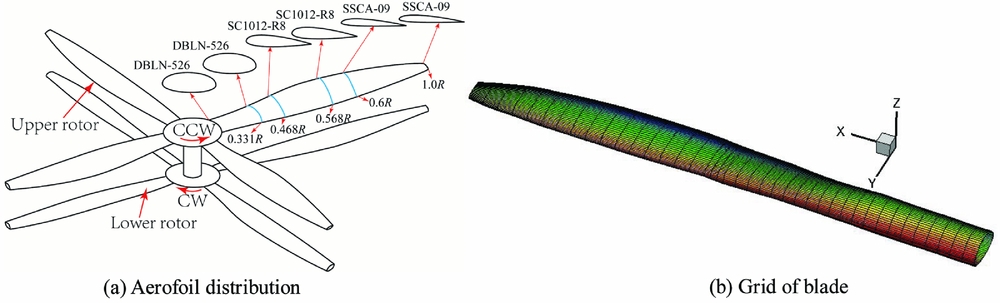
Figure 1. Aerofoil and grid of the coaxial rotor, (a) Aerofoil distribution, (b) Grid of blade.
The aerodynamic model of the coaxial rotor blades is firstly represented using an unsteady panel method(Reference Tan and Wang10). Based on this method, a velocity potential ϕ is defined as
 $$\begin{equation}
\phi (x,y,z,t) = \frac{1}{{4\pi }}\int_{{{S_{\rm{B}}}}}{{{\mu _{\rm{d}}}\bm{n} \cdot \nabla \left( {\frac{1}{\bm{r}}} \right)}}dS - \frac{1}{{4\pi }}\int_{{{S_{\rm{B}}}}}{{\sigma \left( {\frac{1}{\bm{r}}} \right)}}dS + \frac{1}{{4\pi }}\int_{{{S_{\rm{w}}}}}{{{\mu _{\rm{d}}}\bm{n} \cdot \nabla \left( {\frac{1}{\bm{r}}} \right)}}dS
\end{equation}$$
$$\begin{equation}
\phi (x,y,z,t) = \frac{1}{{4\pi }}\int_{{{S_{\rm{B}}}}}{{{\mu _{\rm{d}}}\bm{n} \cdot \nabla \left( {\frac{1}{\bm{r}}} \right)}}dS - \frac{1}{{4\pi }}\int_{{{S_{\rm{B}}}}}{{\sigma \left( {\frac{1}{\bm{r}}} \right)}}dS + \frac{1}{{4\pi }}\int_{{{S_{\rm{w}}}}}{{{\mu _{\rm{d}}}\bm{n} \cdot \nabla \left( {\frac{1}{\bm{r}}} \right)}}dS
\end{equation}$$
where σ and μ d are the source and doublet distributions placed on the blade and wake surfaces, n denotes the outward unit normal vector of a surface, and r is the position vector (x, y, z).
The boundary condition for the blade surfaces requires that the velocity component normal to S B to be zero. A boundary condition of infinity requires the flow disturbance to decrease far away from the rotor owing to the blade's motion through fluid. The boundary condition can then be expressed as
 $$\begin{equation}
\left\{ \begin{array}{@{}l@{}} \frac{{\partial \phi }}{{\partial n}} - {\bm{v}_B} \cdot \bm{n} = 0\quad \quad \quad {\rm{blade}}\;{\rm{surface}}\\ \lim \nabla {\phi _{r \to \infty }} = 0\quad \quad \quad {\hbox{infinite}}\;{\rm{boundary}} \end{array} \right.
\end{equation}$$
$$\begin{equation}
\left\{ \begin{array}{@{}l@{}} \frac{{\partial \phi }}{{\partial n}} - {\bm{v}_B} \cdot \bm{n} = 0\quad \quad \quad {\rm{blade}}\;{\rm{surface}}\\ \lim \nabla {\phi _{r \to \infty }} = 0\quad \quad \quad {\hbox{infinite}}\;{\rm{boundary}} \end{array} \right.
\end{equation}$$
where vB is the velocity of a point on blade surface S B and n denotes the outward unit normal vector at this point. Moreover, r is the position vector (x, y, z). The infinite boundary condition is automatically fulfilled through Green's function.
2.2 Reversed-flow model
In the aerodynamic model of a single rotor blade based on an unsteady panel method, the wake shedding from the trailing edge of the aerofoil at all azimuth locations, including the retreating side, is modelled with the trailing-edge Kutta condition. The model is suitable to represent the aerodynamics of a rotor blade, because the reversed flow is limited to a small area on the retreating side due to the limited maximum forward speed, and thus has weak influence on the aerodynamic airloads in the single rotor. However, as flight speed increases, the reversed flow on the retreating side on both the upper and lower rotors may expand to 0.5R. Also, unlike the single rotor, flow attachment on the retreating side of the coaxial rotor system is observed. As a result, the blade section corresponding to the reversed flow also produces some lift, and can be modelled by the panel method. Additionally, the vortex shedding from the reversed flow will interact with other blades of the upper and lower rotors resulting in unsteadiness of the aerodynamic loads for a coaxial rotor system. Therefore, a reversed flow model is taken into account and coupled into the aerodynamic model of coaxial rotor in the present work.
It is assumed that the flow convects from the leading edge to the trailing edge on the advancing side, and the Kutta condition at the trailing edge is satisfied. Therefore, wake doublets can be expressed in terms of the unknown surface doublet through the trailing-edge Kutta condition. Defining upper and lower trailing-edge (T.E.) doublets as μTEu and μTEd, respectively, the T.E. wake doublet μTEw is given by
 $$\begin{equation}
\mu _w^{TE} = \mu _u^{TE} - \mu _d^{TE}
\end{equation}$$
$$\begin{equation}
\mu _w^{TE} = \mu _u^{TE} - \mu _d^{TE}
\end{equation}$$
However, as opposed to the advancing side, the vortex is shed from the leading edge in the reversed flow on the retreating side of the coaxial rotor. Because of the flow attachment on the retreating side, it is assumed that the leading-edge Kutta condition is satisfied, as shown in Fig. 2. Therefore, the wake doublets can be expressed in terms of the unknown surface doublet through the leading-edge Kutta condition. Defining the upper and lower leading-edge (L.E.) doublets as μLEu and μLEd, respectively, the L.E. wake doublet μLEw is given as
 $$\begin{equation}
\mu _w^{LE} = \mu _u^{LE} - \mu _d^{LE}
\end{equation}$$
$$\begin{equation}
\mu _w^{LE} = \mu _u^{LE} - \mu _d^{LE}
\end{equation}$$
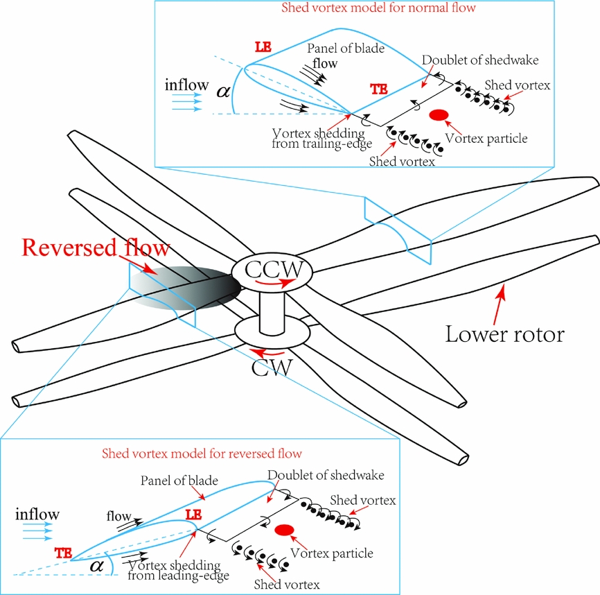
Figure 2. Reversed flow model of the coaxial rotor system.
The potential inside the blade (without internal singularities) will not change for an enclosed boundary (e.g., S B). Therefore, the internal potential is set to ϕint = 0.
 $$\begin{equation}
\frac{1}{{4\pi }}\int_{{{S_{\rm{B}}}}}{{{\mu _{\rm{d}}}\bm{n} \cdot \nabla \left( {\frac{1}{r}} \right)}}dS - \frac{1}{{4\pi }}\int_{{{S_{\rm{B}}}}}{{\sigma \left( {\frac{1}{r}} \right)}}dS + \frac{1}{{4\pi }}\int_{{{S_{\rm{w}}}}}{{{\mu _{\rm{d}}}\bm{n} \cdot \nabla \left( {\frac{1}{r}} \right)}}dS = 0
\end{equation}$$
$$\begin{equation}
\frac{1}{{4\pi }}\int_{{{S_{\rm{B}}}}}{{{\mu _{\rm{d}}}\bm{n} \cdot \nabla \left( {\frac{1}{r}} \right)}}dS - \frac{1}{{4\pi }}\int_{{{S_{\rm{B}}}}}{{\sigma \left( {\frac{1}{r}} \right)}}dS + \frac{1}{{4\pi }}\int_{{{S_{\rm{w}}}}}{{{\mu _{\rm{d}}}\bm{n} \cdot \nabla \left( {\frac{1}{r}} \right)}}dS = 0
\end{equation}$$
By dividing the coaxial rotor blade surface into N panels and wake surface into N w panels, integration on the surfaces in Equation (5) can be equivalently written as the superposition of integrations on the panels that constitute those surfaces. Quadrilateral geometry, constant-strength panels are used in the current study. Thus, Equation (5) can be rewritten as
 $$\begin{equation}
\sum\limits_{k = 1}^N {{\mu _{{\rm{d,}}k}}{A_k}} = - \sum\limits_{k = 1}^N {{\sigma _k}{B_k}} ,
\end{equation}$$
$$\begin{equation}
\sum\limits_{k = 1}^N {{\mu _{{\rm{d,}}k}}{A_k}} = - \sum\limits_{k = 1}^N {{\sigma _k}{B_k}} ,
\end{equation}$$
where Ak includes contributions of the blade surface as well as of the rotor wake surface, and Ak and Bk can be computed using analytical formulations for a constant strength of potential distribution on each panel. The Ak is given as
 \fontsize{10}{12} \selectfont{$$\begin{equation}
{A_k} =\! \left\{\!\! \begin{array}{l@{\quad}l} \frac{1}{{4\pi }}\int_{{{\rm{blade}}}}{{{{{\bf n}}_k} \cdot \nabla (1/\left| {{{{\bf r}}_k}} \right|){\rm{d}}{s_{\rm{k}}}}} &\! k \ne LE\;\;\, {\rm{or}}\;\;\, TE\\[4pt] \frac{1}{{4\pi }}\int_{{{\rm{blade}}}}{{{{{\bf n}}_k} \cdot \nabla (1/\left| {{{{\bf r}}_k}} \right|){\rm{d}}{s_{\rm{k}}}}} \pm \frac{1}{{4\pi }}\int_{{TE{\rm{wake}}}}{{{{{\bf n}}_{TE}} \cdot \nabla (1/\left| {{{{\bf r}}_{TE}}} \right|){\rm{d}}{s_{{\rm{TE}}}}}} &\! k = TE\\[4pt] \frac{1}{{4\pi }}\int_{{{\rm{blade}}}}{{{{{\bf n}}_k} \cdot \nabla (1/\left| {{{{\bf r}}_k}} \right|){\rm{d}}{s_{\rm{k}}}}} \pm \frac{1}{{4\pi }}\int_{{LE{\rm{wake}}}}{{{{{\bf n}}_{LE}} \cdot \nabla (1/\left| {{{{\bf r}}_{LE}}} \right|){\rm{d}}{s_{{\rm{LE}}}}}} &\! k = LE \end{array} \right.,
\end{equation}$$}
\fontsize{10}{12} \selectfont{$$\begin{equation}
{A_k} =\! \left\{\!\! \begin{array}{l@{\quad}l} \frac{1}{{4\pi }}\int_{{{\rm{blade}}}}{{{{{\bf n}}_k} \cdot \nabla (1/\left| {{{{\bf r}}_k}} \right|){\rm{d}}{s_{\rm{k}}}}} &\! k \ne LE\;\;\, {\rm{or}}\;\;\, TE\\[4pt] \frac{1}{{4\pi }}\int_{{{\rm{blade}}}}{{{{{\bf n}}_k} \cdot \nabla (1/\left| {{{{\bf r}}_k}} \right|){\rm{d}}{s_{\rm{k}}}}} \pm \frac{1}{{4\pi }}\int_{{TE{\rm{wake}}}}{{{{{\bf n}}_{TE}} \cdot \nabla (1/\left| {{{{\bf r}}_{TE}}} \right|){\rm{d}}{s_{{\rm{TE}}}}}} &\! k = TE\\[4pt] \frac{1}{{4\pi }}\int_{{{\rm{blade}}}}{{{{{\bf n}}_k} \cdot \nabla (1/\left| {{{{\bf r}}_k}} \right|){\rm{d}}{s_{\rm{k}}}}} \pm \frac{1}{{4\pi }}\int_{{LE{\rm{wake}}}}{{{{{\bf n}}_{LE}} \cdot \nabla (1/\left| {{{{\bf r}}_{LE}}} \right|){\rm{d}}{s_{{\rm{LE}}}}}} &\! k = LE \end{array} \right.,
\end{equation}$$}
 $$\begin{equation}
{B_k} = - \frac{1}{{4\pi }}\int_{{{\rm{blade}}}}{{(1/\left| {{{{\bf r}}_k}} \right|){\rm{d}}{s_{\rm{k}}}}}
\end{equation}$$
$$\begin{equation}
{B_k} = - \frac{1}{{4\pi }}\int_{{{\rm{blade}}}}{{(1/\left| {{{{\bf r}}_k}} \right|){\rm{d}}{s_{\rm{k}}}}}
\end{equation}$$
The conversion of doublet panels of the leading edge to vortex wake in the reversed flow is realised following the coupled method in Reference Tan and WangRef. 10 where the flow induced by a dipole surface distribution μ d defined on a surface S is equivalent to a surface term involving surface vorticity n × ∇μd and a line vortex term μ d over the boundary of the surface. The vortex wake in the surface centre is obtained by integrating the surface vorticity throughout the wake panel and the line vortex bounding the surface.
2.3 Effect of vortex-blade aerodynamic interaction
The interaction of the upper rotor wake with the lower rotor, along with that between tip vortices from the two rotors with each other and the inboard sheet, produce a highly complicated flow field and unsteady airloads. Consequently, the unsteadyness of the coaxial rotor wake should to be taken into account in the prediction of rotor loads. Based on the panel method as mentioned before, the unsteady pressure on the blade surfaces can be calculated using the velocity potential and flow velocity through Bernoulli's equation.
 $$\begin{equation}
\frac{{\partial \phi }}{{\partial t}} + \frac{1}{2}{{v}^2} + \frac{1}{\rho }p = \frac{1}{\rho }{p_{{\rm{ref}}}}
\end{equation}$$
$$\begin{equation}
\frac{{\partial \phi }}{{\partial t}} + \frac{1}{2}{{v}^2} + \frac{1}{\rho }p = \frac{1}{\rho }{p_{{\rm{ref}}}}
\end{equation}$$
The vortex of the upper rotors impinges on the blade surface of the lower rotor resulting in a variation of the unsteady term ∂ϕ/∂t in Equation (9) and in an unsteady pressure response, especially for blade vortex interaction (BVI). It is believed that the interaction between the coaxial rotor systems plays a significant role in the amount of unsteadiness of the airloads, and should be taken into account in the prediction of the time-varying airloads. Therefore, the effect of vortex-blade aerodynamic interaction is modelled thought the unsteady pressure term induced by the coaxial-rotor wake and both rotor blades. Thus, the non-dimensionalised form of the blade unsteady pressure is then given as
 $$\begin{equation}
\begin{array}{@{}l@{}} C_p^{\rm{u}} = \frac{{{p^{\rm{u}}} - {p_{{\rm{ref}}}}}}{{\left( {1/2} \right)\rho {{\left( {{v}_{{\rm{ref}}}^{\rm{u}}} \right)}^2}}} = 1 - \frac{{{{\left( {{v}_{\rm{B}}^{\rm{u}}} \right)}^2}}}{{{{\left( {{v}_{{\rm{ref}}}^{\rm{u}}} \right)}^2}}} - \frac{2}{{{{\left( {{v}_{{\rm{ref}}}^{\rm{u}}} \right)}^2}}}\left( {\frac{{\partial \phi _{\rm{b}}^{\rm{l}}}}{{\partial t}} + \frac{{\partial \phi _{\rm{w}}^{\rm{l}}}}{{\partial t}}} \right)\\[9pt] C_p^l = \frac{{{p^{\rm{l}}} - {p_{{\rm{ref}}}}}}{{\left( {1/2} \right)\rho {{\left( {{v}_{{\rm{ref}}}^{\rm{l}}} \right)}^2}}} = 1 - \frac{{{{\left( {{v}_{\rm{B}}^{\rm{l}}} \right)}^2}}}{{{{\left( {{v}_{{\rm{ref}}}^{\rm{l}}} \right)}^2}}} - \frac{2}{{{{\left( {{v}_{{\rm{ref}}}^{\rm{l}}} \right)}^2}}}\left( {\frac{{\partial \phi _{\rm{b}}^{\rm{u}}}}{{\partial t}} + \frac{{\partial \phi _{\rm{w}}^{\rm{u}}}}{{\partial t}}} \right) \end{array},
\end{equation}$$
$$\begin{equation}
\begin{array}{@{}l@{}} C_p^{\rm{u}} = \frac{{{p^{\rm{u}}} - {p_{{\rm{ref}}}}}}{{\left( {1/2} \right)\rho {{\left( {{v}_{{\rm{ref}}}^{\rm{u}}} \right)}^2}}} = 1 - \frac{{{{\left( {{v}_{\rm{B}}^{\rm{u}}} \right)}^2}}}{{{{\left( {{v}_{{\rm{ref}}}^{\rm{u}}} \right)}^2}}} - \frac{2}{{{{\left( {{v}_{{\rm{ref}}}^{\rm{u}}} \right)}^2}}}\left( {\frac{{\partial \phi _{\rm{b}}^{\rm{l}}}}{{\partial t}} + \frac{{\partial \phi _{\rm{w}}^{\rm{l}}}}{{\partial t}}} \right)\\[9pt] C_p^l = \frac{{{p^{\rm{l}}} - {p_{{\rm{ref}}}}}}{{\left( {1/2} \right)\rho {{\left( {{v}_{{\rm{ref}}}^{\rm{l}}} \right)}^2}}} = 1 - \frac{{{{\left( {{v}_{\rm{B}}^{\rm{l}}} \right)}^2}}}{{{{\left( {{v}_{{\rm{ref}}}^{\rm{l}}} \right)}^2}}} - \frac{2}{{{{\left( {{v}_{{\rm{ref}}}^{\rm{l}}} \right)}^2}}}\left( {\frac{{\partial \phi _{\rm{b}}^{\rm{u}}}}{{\partial t}} + \frac{{\partial \phi _{\rm{w}}^{\rm{u}}}}{{\partial t}}} \right) \end{array},
\end{equation}$$
where p ref and ρ are far-field reference pressure and density, v uB, p u, v uref are the local fluid velocity, local pressure, the reference velocity, respectively, at each section of the upper rotor, while v lB, p l, v lref are the local fluid velocity, local pressure, the reference velocity, respectively, at each section of the lower rotor. Also, ϕub and ϕuw are the velocity potential induced by the upper rotor blades and its wake, respectively, whereas ϕlb and ϕlw are the velocity potential induced by the lower rotor blades and its wake, respectively.
The unsteady pressure term induced by both rotor blades can be directly described by the derivative of velocity potential, whilst that of the coaxial-rotor wake can be transformed into the product of induced velocity from wake and velocity of wake (induced velocity from vortex particles and velocity of vortex particles), which is similar to the effect of tip-vortex filaments(Reference Lorber and Egolf17). Those derivatives of velocity potential can be expressed as
 $$\begin{equation}
\begin{array}{@{}l@{}} \partial \phi _{\rm{b}}^{\rm{u}}/\partial t = (\phi _{\rm{b}}^{{\rm{u}},t} - \phi _{\rm{b}}^{{\rm{u}},t - \Delta t})/\Delta t\\[4pt] \partial \phi _{\rm{b}}^{\rm{l}}/\partial t = (\phi _{\rm{b}}^{{\rm{l}},t} - \phi _{\rm{b}}^{{\rm{l}},t - \Delta t})/\Delta t \end{array},
\end{equation}$$
$$\begin{equation}
\begin{array}{@{}l@{}} \partial \phi _{\rm{b}}^{\rm{u}}/\partial t = (\phi _{\rm{b}}^{{\rm{u}},t} - \phi _{\rm{b}}^{{\rm{u}},t - \Delta t})/\Delta t\\[4pt] \partial \phi _{\rm{b}}^{\rm{l}}/\partial t = (\phi _{\rm{b}}^{{\rm{l}},t} - \phi _{\rm{b}}^{{\rm{l}},t - \Delta t})/\Delta t \end{array},
\end{equation}$$
 $$\begin{equation}
\begin{array}{@{}l@{}} \partial \phi _{\rm{w}}^{\rm{u}}/\partial t = - \sum {{v}_{{\rm{ind}}}^{\rm{u}}({{x}_{\rm{u}}}) \cdot {v}_{\rm{w}}^{\rm{l}}({{{x'}}_{\rm{l}}})} \\[4pt] \partial \phi _{\rm{w}}^{\rm{l}}/\partial t = - \sum {{v}_{{\rm{ind}}}^{\rm{l}}({{x}_{\rm{l}}}) \cdot {v}_{\rm{w}}^{\rm{u}}({{{x'}}_{\rm{u}}})} \end{array},
\end{equation}$$
$$\begin{equation}
\begin{array}{@{}l@{}} \partial \phi _{\rm{w}}^{\rm{u}}/\partial t = - \sum {{v}_{{\rm{ind}}}^{\rm{u}}({{x}_{\rm{u}}}) \cdot {v}_{\rm{w}}^{\rm{l}}({{{x'}}_{\rm{l}}})} \\[4pt] \partial \phi _{\rm{w}}^{\rm{l}}/\partial t = - \sum {{v}_{{\rm{ind}}}^{\rm{l}}({{x}_{\rm{l}}}) \cdot {v}_{\rm{w}}^{\rm{u}}({{{x'}}_{\rm{u}}})} \end{array},
\end{equation}$$
where x u, v uw, x'u are blade position, velocity and position of tip vortex of the upper rotor, respectively, while x l, v lw, x'l are blade position, velocity and position of tip vortex of the lower rotor, respectively. v uind and v lind are velocity of the upper rotor induced by the lower rotor tip vortex and velocity of the lower rotor induced by the upper rotor tip vortex, respectively.
The aerodynamic airloads on the panels of both the upper and lower rotors can be then computed as
 $$\begin{equation}
\Delta {{F}_k} = - {C_{pk}}{\left( {\rho {v}_{{\rm{ref}}}^2/2} \right)_k}\Delta {S_k}{{n}_k},
\end{equation}$$
$$\begin{equation}
\Delta {{F}_k} = - {C_{pk}}{\left( {\rho {v}_{{\rm{ref}}}^2/2} \right)_k}\Delta {S_k}{{n}_k},
\end{equation}$$
where ΔFk is the aerodynamic load on the panel, ΔSk is the panel area, and n k is its normal vector.
2.4 Wake model of the coaxial-rotor system
Vortex shedding from the coaxial rotor system may directly induce an unsteady pressure response and affect the rotor tip vortex. Therefore, simulating the coaxial rotor wake plays a significant role in predicting the unsteady airloads of the coaxial system. The wake of the coaxial rotor system shown in Fig. 3 is modelled using a viscous vortex particle method(Reference Tan and Wang10) which solves the Navier-Stokes equation with velocity-vorticity (u, ω) in a Lagrangian frame by using vector-valued particles.
 $$\begin{equation}
\frac{{\partial {\omega }}}{{\partial t}} + {u} \cdot \nabla {\omega } = \nu {\nabla ^2}{\omega } + \nabla {u} \cdot {\omega }
\end{equation}$$
$$\begin{equation}
\frac{{\partial {\omega }}}{{\partial t}} + {u} \cdot \nabla {\omega } = \nu {\nabla ^2}{\omega } + \nabla {u} \cdot {\omega }
\end{equation}$$
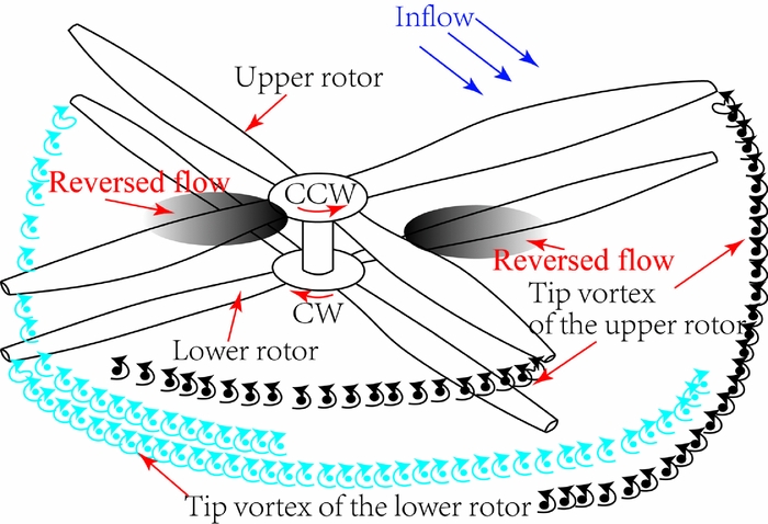
Figure 3. Tip vortex of the coaxial rotor.
The right-hand-side term describes vortex particle convection which is solved by using a fourth-order Runge-Kutta scheme, and the left-hand-side term expresses the viscous diffusion and stretching effect. The viscous diffusion effect is simulated through the particle strength exchange (PSE), and the vortex stretching effect is represented by a direct scheme.
The trailing-edge and leading-edge vortices are shed from the surface of the coaxial rotor blade through a Neumann boundary condition and by converting shed-wake doublet panels to wake vorticity. After then, it convects based on Equation (14).
3.0 NUMERICAL RESULTS AND DISCUSSSION
3.1 Unsteady airloads of coaxial-rotor system
The X2TD model is computed in forward flight. This coaxial rotor has eight blades of non-uniform chord and non-linear twist. The rotor radius is 4.023m and the tip hover Mach number is 0.554. The aerofoil distribution with the DBLN-526, SC1012-R8, SSCA-09 scheme is shown in Fig. 1. The blade is modelled with 19200 panels composed of 60 panels in the chordwise direction and 40 panels in the spanwise direction. The azimuthal angle step is 2.5°.
Figure 4 shows the variation in the sectional thrust coefficient at characteristic radial stations over one revolution at different flight speeds, μ = 0.15, 0.27, and 0.41. Note that, when viewed from above, the upper rotor rotates in an anti-clockwise fashion and the lower rotor rotates clockwise. Therefore, to clearly plot and compare the variation of the sectional airloads, the azimuthal locations of the upper and lower rotors are measured in the rotational direction of the upper rotor. The present results are also compared with results of PRASADUM and full grid-based CFD results(Reference Passe, Sridharan and Baeder13) found in the literature. In the PRASADUM solver, blade section aerodynamics based on a lifting-line method was modelled using look-up tables with quasi-steady and non-circulatory corrections for aerofoil pitch and plunge motions. Also, two inflow models, the finite-state dynamic inflow and the Maryland free wake, were integrated into the solver to account for the influence of the coaxial-rotor wake. The CFD solvers of the CREATE AV Helios framework include OVERFLOW, and overset meshes can be used to simulate aerodynamic interactions.
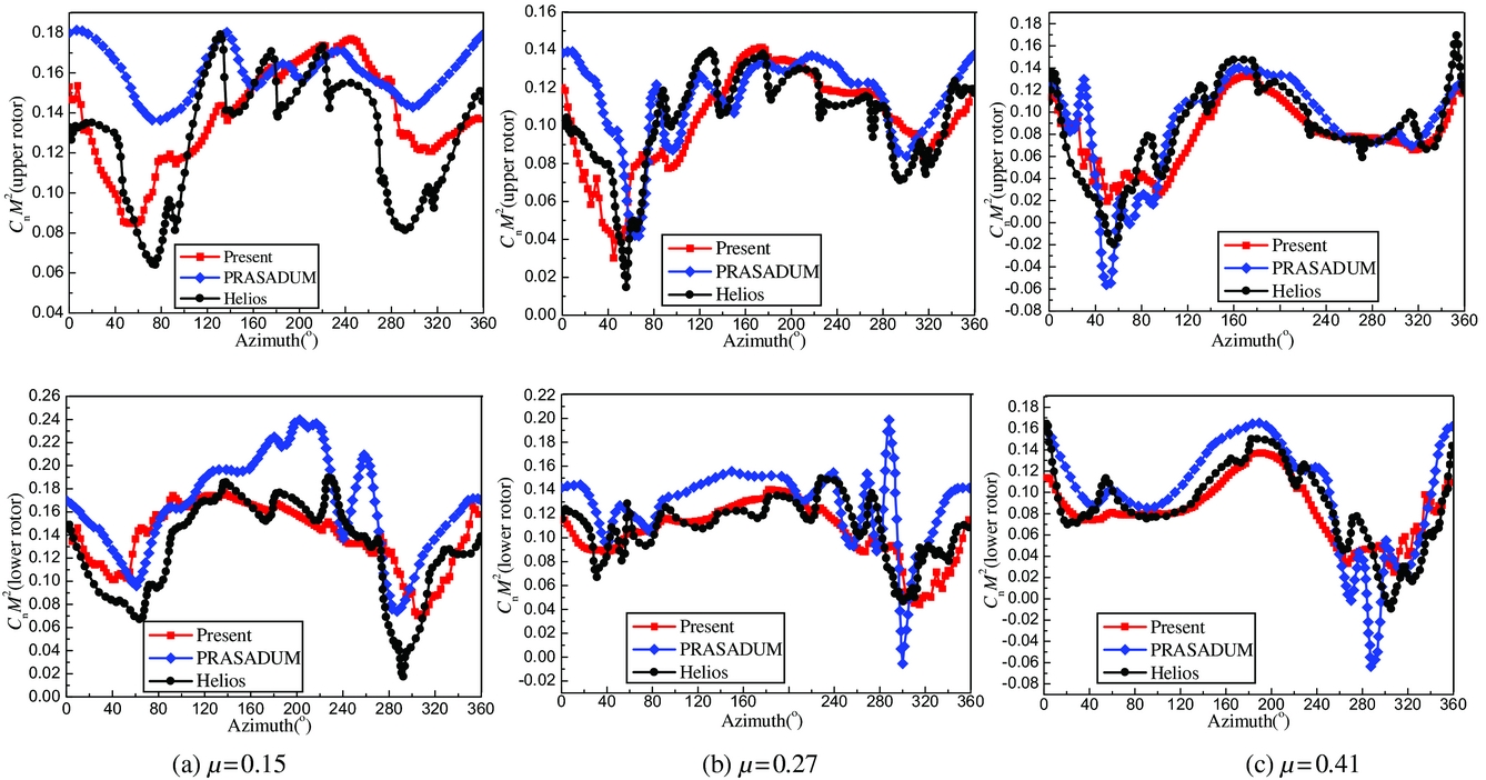
Figure 4. Sectional airloads of the coaxial rotor at different forward speeds, (a) μ = 0.15, (b) μ = 0.27, (c) μ=0.41.
The variations of the sectional thrust coefficient at different flight speeds in the present simulation correlate well with those found in the CFD results of Helios near azimuthal angles of 60° and 300°. Furthermore, the thrust coefficient is also in accordance with CFD results in terms of magnitude and phase. Additionally, the influence of the interaction between the coaxial rotor wake and the blades on the sectional thrust distributions is observed on the advancing side at azimuth angles of around 40–120° and on the retreating side at around 260–320°. The present predictions and the results of PRASADUM show similar trends as the CFD results at different flight speeds. However, at low-speed flight, the unsteady airloads are under-predicted by the PRASADUM on the advancing side at azimuthal angles of around 40–120° and on the retreating side at around 260–320°, while at high-speed flight, over-predictions occur. Moreover, the airloads of the lower rotor were also over-predicted at different flight speeds. Therefore, compared with the PRASADUM results, the predicted fluctuations of sectional thrust agree better with the CFD results on the advancing side at azimuthal angles of around 40–120° and on the retreating side at around 260–320°. It should be noted that even though there are some discrepancies in the present prediction, the overall comparison is still good and the results of the present method are found to match well with the results of the CFD/CSD method. Moreover, the simulation in the CFD is run for eight revolutions to converge. The runtime corresponds to 9600 CPU hours on the AFRL and ARL HPC clusters parallelised through MPI using 240 processors. However, the computer time with eight revolutions in the present prediction is about 155 CPU hours on a desktop using only one CPU of Intel i7-3770 3.4GHz. Therefore, contrary to the grid-based CFD, the present method estimating the unsteady airloads is more efficient.
3.2 Differential aerodynamic loads between the upper and lower rotor
The azimuthal distribution of unsteady airloads on the upper and lower rotors of Fig. 5 provides some insight into the difference of the airloads on the coaxial rotor blades. Comparing the airloads of the upper rotor at low forward speed, it can be seen that the airloads of the lower rotor reduce visibly on the advancing side at azimuthal angles of around 40–120° and on the retreating side at around 260–320°, especially at an azimuthal angle of 300°. This is a result of the interaction between the wakes of the coaxial rotor blades. Additionally, as expected, the tip vortex of the upper rotor impinges on the lower rotor as shown in Fig. 6. Note that in this graph, the tip vortex of the upper rotor is indicated with red, while the tip vortex of the lower rotor is indicated with blue. Moreover, the lower rotor blade on the advancing side at azimuthal angles of around 40–120° and on the retreating side around 260–320° are affected by the rolled-up tip vortex of the upper rotor which results in a decrease of the angle-of-attack.
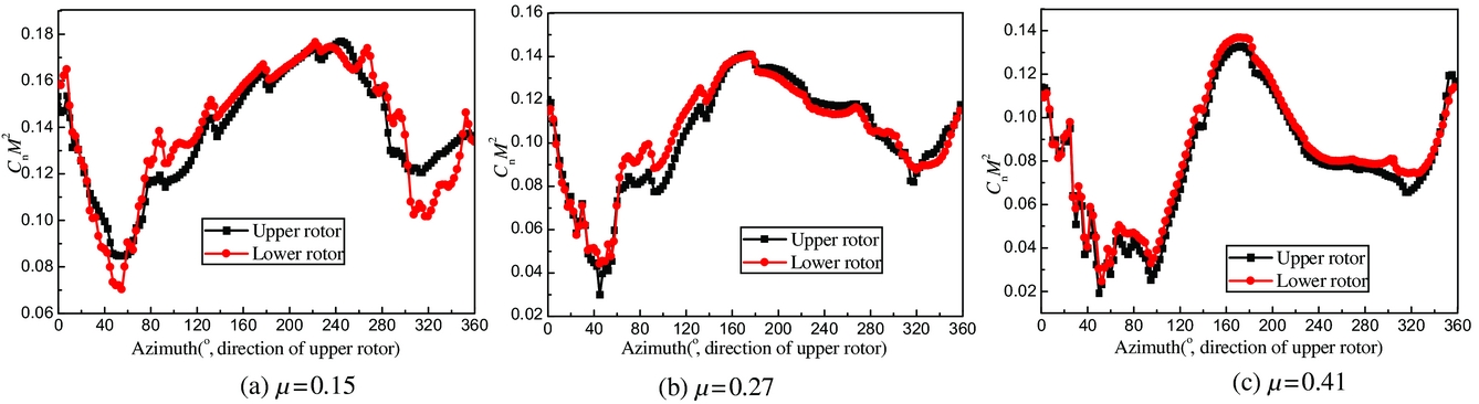
Figure 5. Sectional airload of the upper and lower rotors, (a) μ = 0.15, (b) μ = 0.27, (c) μ = 0.41.

Figure 6. Rotor wake of the coaxial rotor at different forward speeds, (a) μ = 0.15, (b) μ = 0.27, (c) μ = 0.41.
As flight speed increases, the difference in airloads between the upper and lower rotors decreases as shown in Fig. 5. This is because, the rotor wake at high advance ratio is swept away quickly and the angle-of-attack between the upper and lower rotors is quite similar. In addition, it is observed in Fig. 6 that the tip vortex of the upper rotor swept above the lower rotor resulting in a weakening of the interaction between the upper and lower rotor wakes.
The distributed inflows of the upper and lower rotors at two different forward speeds, μ = 0.15 and 0.41, are shown in Fig. 7. As mentioned before, the rotor wake at low speed convects downwards and impinges on the lower rotor, resulting in a reduction of inflow on the advancing side at azimuthal angles of 40–120°, and on the retreating side at 260–320°. As a result, the blade vortex interaction is obvious on the advancing side at azimuthal angles of around 40–120° and on the retreating side at around 260–320° which is shown in Fig. 7(c). However, the difference of inflow between the upper and lower rotors decreases as the flight speed increases. Also, the reduced inflow due to blade vortex interaction disappears, and the influence of vortex interaction between the upper and lower rotors is alleviated as the rotor wake swept away quickly.

Figure 7. Induced velocity of the coaxial rotor, (a) Upper rotor (μ = 0.15), (b) Lower rotor (μ = 0.15), (c) Difference (μ = 0.15), (d) Upper rotor (μ = 0.41), (e) Lower rotor (μ = 0.41), (f) Difference (μ = 0.41).
Figure 8 presents the distribution of forces for the upper and lower rotors at two different forward speeds. At low forward speed, the area of reversed flow is small and the lift off-set is also limited. Therefore, the forces on the forward and backward parts of the rotor plan are obvious and shown in Fig. 8(a) and (b). It is worth noting that in this graph, the difference in forces between the upper and lower rotors is striped on the advancing and retreating side due to the tip vortex of the upper rotor impinging on the lower rotor as mentioned earlier. This fluctuation of forces indicates the influence of blade-vortex interaction on the coaxial rotor system. In addition, the differences in force on the retreating side at the azimuth of 260–320° is most important because of the obvious reduction of inflow induced by the tip vortex of the upper rotor.

Figure 8. Sectional force of the coaxial rotor, (a) Upper rotor (μ=0.15), (b) Lower rotor (μ=0.15), (c) Difference (μ=0.15), (d) Upper rotor (μ=0.41), (e) Lower rotor (μ=0.41), (f) Difference (μ=0.41).
As the flight speed increases, the reversed flow expands and the lift-off-set increases. As a result, the force on the advancing side is the dominant component of rotor thrust for both the upper and lower rotors. Furthermore, with increasing speed, the difference of force on the advancing and retreating side due to the tip vortex interaction between the upper and lower rotors decreases, while the difference of force corresponding to the effect of blade passage increases. It can be seen that the difference in force shows 8/rev unsteady loads. This is because both the upper and lower rotor wakes move downstream quickly, resulting in weakened interactions between the two-rotor system. However, as the blades of the upper and lower rotors approach each other, an upwash on each blade is induced. It initially increases as the blades approach, and then begins to decrease and changes sign thus representing a downwash as the blades leave. The downwash increases and then starts decreasing when the blades move away from each other. As a result, the forces on the upper and lower rotors increase as the blades approach, then decrease and then increase again as they move away from each other.
The wake visualisation of the coaxial rotor at low speed, μ = 0.15, is shown in Fig. 9. The iso-surface is coloured by the sense of the vorticity vector. Similar to the single rotor, the tip vortices trailing behind the blades tangle around one another and roll up along the rotor on the advancing and retreating sides, and the fully rolled-up vorticity structure is well defined and discrete. The fully rolled-up vorticity structure is similar to the tip vortex observed behind a single rotor and fixed-wing aircraft. However, it is interesting to note that the tip vortices from the upper and lower rotor blades interact with each other and produce two coherent rolled-up bundles. At the first instance, the tip vortex of the upper rotor, indicated as ①, is above the tip vortex of the lower rotor, indicated as ②. At a later time, the tip vortex ① shed from the upper blades contracts in the radial direction and convects down owing to the induced velocity of the lower rotor tip vortex ② at x = 0.5R-0.75R result in the upper rotor wake structure impinging on the lower rotor, while the tip vortex ② is pushed upstream due to induced effect of the upper rotor tip vortex ①. As a result, the tip vortex ② comes to contact with the tip vortex ① under their mutually-induced effect and the tip vortex ① changes position with the tip vortex ② resulting in two coherent rolled-up bundles. Moreover, it is also observed that the tip vortex of the upper rotor contracts faster in the radial direction compared to that of the lower rotor caused by the influence of roll-up vortex of the lower rotor.

Figure 9. Interchange of tip vortex position of the coaxial rotor (μ = 0.15), (a) Wake structure, (b) x = 0.25R, (c) x = 0.5R, (d) x = 0.75R, (e) x = 1.0R, (f) x = 1.25R.
The azimuthal distribution and frequency of the induced flow and sectional thrust coefficient at a radial station, r/R = 0.75, in Fig. 10 provides insight into the effect of the tip vortex interaction between the upper and lower rotors. The induced inflow at azimuth of 80–240° for the upper and lower rotors is similar. However, the induced inflow of the lower rotor on the advancing side at azimuth of 0–80°and on the retreating side at azimuth of 240–360° is more serious than that of the upper rotor due to tip vortex interaction of the lower rotor. Furthermore, the tip vortex interaction causes not only a 17.5% increase in the 1/rev component but also yields a 30.9%, 144.2%, 194.7% increase in the 3/rev, 4/rev, 5/rev components, respectively. In addition, the 3/rev, 4/rev, 5/rev component of the unsteady airloads for the lower rotor also increase compared to that of the upper rotor.
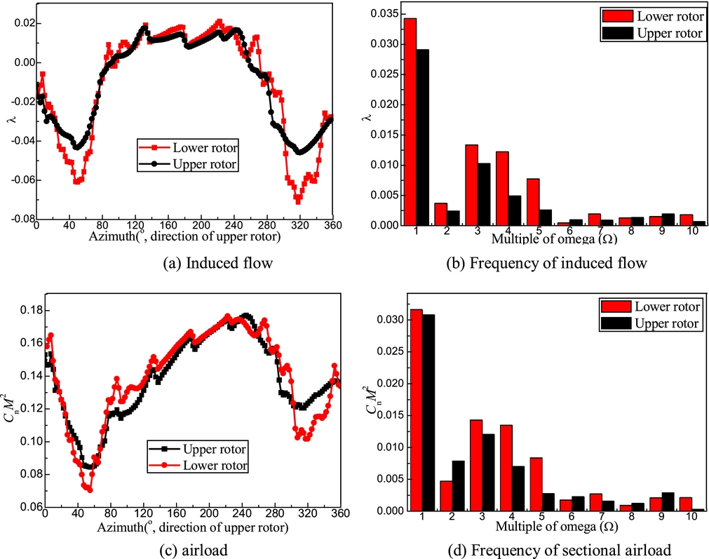
Figure 10. Frequency of sectional airload and induced flow of the coaxial rotor (μ = 0.15), (a) Induced flow, (b) Frequency of induced flow, (c) airload, (d) Frequency of sectional airload.
3.3 Differential aerodynamic loads between coaxial and single rotor
Figure 11 shows the azimuthal distribution of sectional thrust coefficient for the coaxial and single rotors at three flight speeds. The geometry and control scheme of the single rotor are identical to the coaxial rotor to analyse the different airloads at the same conditions. Clearly, as opposed to the single-rotor system, the sectional thrust coefficient on the advancing side at azimuthal angles of 60° and on the retreating side at 300° is obviously smaller because of the influence of the tip vortex of the other rotor. This is because the upper rotor tip vortex at low speed impinges on the lower rotor resulting in a reduction of inflow on the advancing side at azimuthal angles of around 40–120° and on the retreating side at around 260–320°, while the inflow of single rotor is only affected by its own tip vortex. As a result, the sectional thrust coefficient reduces. This suggests that, contrary to the single rotor system, the tip vortex interaction between the upper and lower rotors is comparable or even predominant. However, the difference of sectional thrust coefficient between the coaxial and single rotors decreases with increasing flight speed. This is because the tip vortex convects downstream quickly and the interaction of the upper and lower rotors weakens.
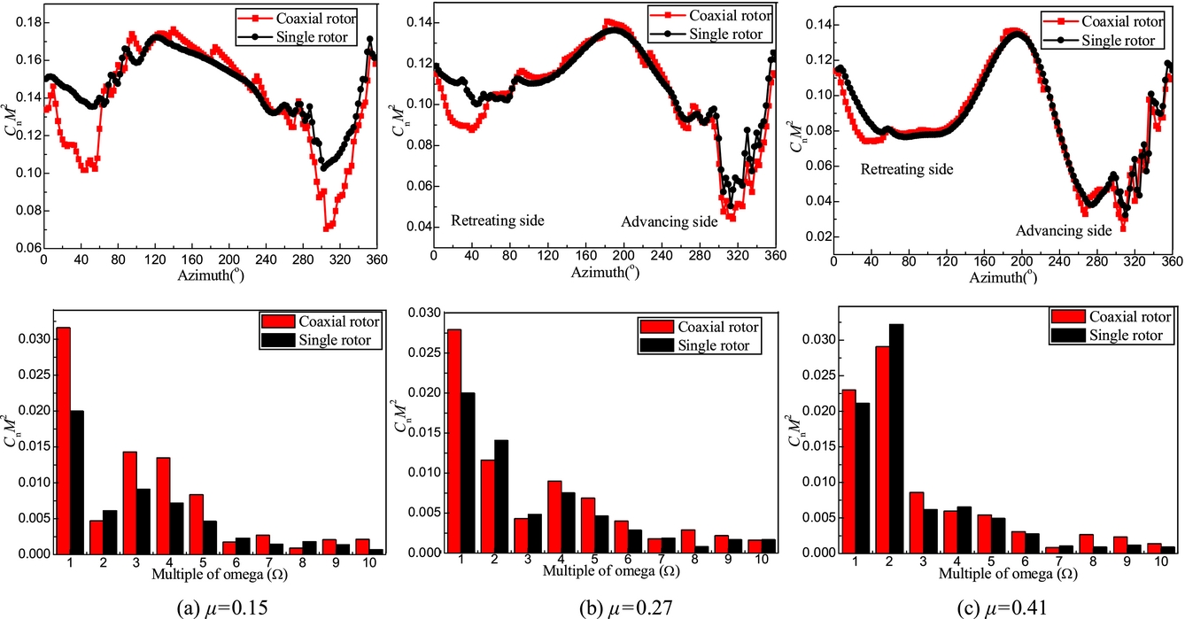
Figure 11. Sectional airload and frequency of the coaxial and single rotors, (a) μ = 0.15, (b) μ = 0.27, (c) μ = 0.41.
The frequencies of sectional thrust coefficients for the coaxial and single rotors at three flight speeds are also shown in Fig. 11 which shows that, contrary to the single rotor, the 1/rev, 3–10/rev components of thrust coefficient on the coaxial rotor obviously increase. However, the difference of 1/rev component decreases with increasing flight speed. The reason for the differences is explained by the tip vortex interaction on the advancing side at azimuthal angles of 60° and on the retreating side at 300° at low speed which is seen to contribute to the significant increase of the 1/rev component, while the interaction decreases as the flight speed increases. Nevertheless, as the flight speed increases, the 8/rev component of the coaxial rotor is greater than that of single rotor due to the rotor blade passing effect which induces high-frequency, unsteady pressure and is more obvious at high speed flight. For the coaxial rotor, each rotor blade of the lower rotor will meet other blades of the upper rotor eight times, which result in 8/rev component of unsteady airloads.
Figure 12 illustrates the difference of the induced flow and the sectional forces between the coaxial and single rotors. The tip vortex interaction between the coaxial-rotor systems is obviously seen to generate significant fluctuations of inflow and force on the advancing and retreating side at low-speed flight. As the flight speed increases, the effect of the tip vortex interaction of the coaxial rotor is weakened and the fluctuations on the advancing and retreating sides reduce. Additionally, the variation due to blade-passing effect is strengthened. Therefore, the aerodynamic interaction for the coaxial rotor is more serious than for the single rotor. Since the hub of the coaxial rotor which is absent in the present simulation will also generate wake and interact with the coaxial rotor, the effect of the hub on the unsteady airloads of the coaxial rotor will be then analysed in future work.

Figure 12. Change in induced velocity and sectional force due to the single and coaxial rotor, (a) μ = 0.15, (b) μ = 0.27, (c) μ = 0.41.
4.0 CONCLUSIONS
An unsteady aerodynamic analysis method including a reversed flow model for the retreating side of the coaxial rotor, the effect of vortex-blade aerodynamic interaction, and a vortex particle method is developed to simulate the unsteady aerodynamic loads for a coaxial rotor. This includes the aerodynamic interactions between rotors and rotor blades. The unsteady aerodynamic loads on the X2 coaxial rotor are simulated in forward flight, and compared with the results of PRASADUM and published CFD/CSD computations with OVERFLOW and the CREATE-AV Helios tools. The results of the present method agree well with the results of the CFD/CSD method, and compare better than the PRASADUM solutions. Furthermore, comparing the inflow and airloads of the upper rotor at low forward speed, the airloads of the lower rotor reduce on the advancing and retreating sides due to the tip vortex of upper rotor impinging on the lower rotor. The difference in airloads between the upper and lower rotors decreases with increasing flight speed. However, the difference of forces corresponding to the effect of the blade passage increases. Moreover, the tip vortices from the upper and lower rotor blades interact with each other and produce two coherent rolled-up bundles and change position at low speed, while the rotor wake at high advance ratio is swept away quickly resulting in a weakened interaction between both rotors. Additionally, contrary to the single rotor system, the tip vortex interaction between the upper and lower rotors is comparable or even predominant to the difference of the sectional thrust coefficient between the coaxial and single rotors. However, as flight speed increases, the inflow and airloads due to the rotor blade passing effect of the coaxial rotor become more pronounced.
ACKNOWLEGEMENTS
This work was supported by the National Natural Science Foundation of China (Grant No. 11502105), and the support of the Natural Science Foundation of Jiangsu Province (Grant No. BK20161537) and the Jiangsu Government Scholarship for Overseas Studies is gratefully acknowledged.


