


1. Introduction
The metamorphism of dry seasonal snow on the ground is classically described by water-vapour transfer between grains (Reference ColbeckColbeck, 1983a). Depending on the degree of thermodynamic disequilibrium, the microstructure will evolve towards either faceted (Reference YosidaYosida and others, 1955) or rounded grain shapes (Reference ColbeckColbeck, 1983a). Among other things, the formation of facets requires a sustained supersaturation with regard to vapour. In a snow cover, this usually happens where a temperature gradient (TG) exists. The formation of rounded grains, which occurs close to equilibrium (no TG, with a temperature T close to 0 ˚ C), is often called isothermal metamorphism of temperate snow. This is the subject of the present study.
The observed vapour transfer between metamorphosing snow grains results from some coupling of reaction and diffusion processes. As in many problems of kinetics, the macroscopic morphology will show the action of the slowest process: it is said that the problem is limited by this process. The main question is whether isothermal snow metamorphism is either reaction or diffusion-limited.
The diffusion-limited hypothesis is clearly the most popular in the snow science community (see, e.g. Reference ColbeckColbeck, 1997; Reference Legagneux and DominéLegagneux and Dominé, 2005). In ceramic science, most materials of practical interest have a very low saturating vapour pressure p sat at the temperature they are processed. Conversely, the few vapour-grown industrial materials such as SiC are processed under high temperature, low total pressure and high supersaturation, (see, e.g. Reference Chen, Zhang, Ma, Prasad, Balkas and YushinChen and others, 2001). An overview of the SiC bulk growth technique is available at http://www.ifm.liu.se/matephys/new page/research/sic/Chapter3.html#3.1.
Literature on the regime of very low supersaturation for materials at a high partial vapour pressure p vap (typically, for a snow sample at −2 ˚ C, p vap ∼ p sat ∼ 517.3 Pa) is scarce. The reaction coefficient α ∈ [0, 1] is formally defined as the ratio between the number of reacting (adsorbing) and incident molecules on a surface; it is the standard way of addressing the question of reaction vs diffusion (Reference MutaftschievMutaftschiev, 2001). A low value of α implies the growth process is reaction-limited. A high value is related to a diffusion-limited growth, except for vacuum conditions where the mean free path of water vapour compares to the crystal size. Existing measurements of α on ice were often carried out at low temperature (T<−100 ˚ C) and vacuum conditions, forcing a reaction-limited growth, which in turn tells us how to relate the growth rate to α. Regardless, results range within more than two orders of magnitude (Reference BrownBrown and others, 1996).
As an exception, a recent work (Reference LibbrechtLibbrecht, 2003) presents data near 0 ˚ C with low values of α for low supersaturations σ ≡ p vap /p sat − 1. Although such conditions of very low growth rates may lead to higher errors in the determination of α for experimental reasons, this finding would advocate a reaction-limited metamorphism, contrasting with the common assumption (Reference ColbeckColbeck, 1997).
For this reason, three-dimensional (3-D) simulations of snow metamorphism were carried out assuming reaction-limited conditions for isothermal (Reference Flin, Brzoska, Lesaffre, Coléou and PieritzFlin and others, 2003) and TG (Reference Flin, Brzoska, Pieritz, Lesaffre, Coléou, Furukawa and KuhsFlin and others, 2007) metamorphism. The requirement of dealing with extremely low vapour fluxes makes the design of a conclusive experiment very difficult, for example measuring the equilibrium shape of isolated crystals (Reference Eaglesham, White, Feldman, Moriya and JacobsonEaglesham and others, 1993). Here, the results of a simple model of diffusion-limited isothermal metamorphism are presented, then applied to the same 3-D data as the formerly developed reaction-limited model (Reference Flin, Brzoska, Lesaffre, Coléou and PieritzFlin and others, 2003), in order to prepare further intercomparisons between the two approaches.
2. Modelling
2.1. Models for isothermal metamorphism
In low-flux metamorphism at high temperatures (close to 0 ˚ C) and high p sat, the following can be assumed, regardless of the limiting process:
-
1. The mass transfer in the pore phase only occurs by molecular diffusion. There is no convection in snow, even for moderate thermal gradients (Reference Brun and TouvierBrun and Touvier, 1987; Reference Kaempfer, Schneebeli and SokratovKaempfer and others, 2005).
-
2. Heat conduction across the grain phase is the fastest process (Reference Sekerka, Müller, Métois and RudolphSekerka, 2004). The latent heat is quickly removed through the highly conductive ice (Reference ColbeckColbeck, 1983b) and the temperature T is considered constant and uniform in the snow matrix.
-
3. Grain metamorphism is the slowest process. For a given state of the microstructure, steady-state solutions are expected for both vapour diffusion (referred to as diffusion) and sublimation/condensation (referred to as reaction) processes.
-
4. The grain’s interface stays microscopically rough everywhere, i.e. it behaves like a surface of type K (Reference MutaftschievMutaftschiev, 2001) saturated with kinks. Thus we do not expect faceted shapes in high-temperature isothermal metamorphism of snow.
As mentioned in the introduction, two different mechanisms can be assumed to be controlling the isothermal metamorphism: a reaction mechanism at the ice–pore interface and a diffusion mechanism through the pore space. After recalling the main features of the reaction-limited hypothesis, we will focus on the diffusion-limited assumption.
Reaction-limited process
In case of a reaction-limited process, the vapour field is assumed to be constant (steady state) and uniform (fast diffusion) at a value p amb(T) such that no macroscopic vapour flux is observed at the scale of the sample in respect to assumption (1). This happens when vapour is in equilibrium with any infinite surface whose mean curvature κ (n being the unit local normal, κ ≡ (div n)/2) equals the integral mean curvature 〈κ〉 of snow in the sample. The ice surface is considered out of equilibrium with respect to the surrounding uniform pressure field, and its growth is governed by the Langmuir–Knudsen equation that gives the mass vapour flux j vap:
where R and M are the ideal gas constant and molar mass of vapour, respectively. p sat(κ, T ) is given by Kelvin’s law:
where p∞ sat (T ), γ and V spe are the saturating vapour pressure over a macroscopically flat, microscopically rough surface of ice, the ice–vapour surface tension and the specific volume of ice, respectively. If the curvature field is available on a sample, local growth rates can be computed in a straightforward manner. This made early simulations of metamorphism possible (Reference Flin, Brzoska, Lesaffre, Coléou and PieritzFlin and others, 2003).
Diffusion-limited process
In the present paper, the metamorphism is assumed to be limited by a vapour diffusion process. In the pore space, p vap should obey the stationary equation of diffusion:
where r is the position vector. The grain surface S is considered to be in equilibrium with the vapour, at a uniform and constant temperature T . This provides a Dirichlet boundary condition to the vapour field, i.e.
After solving Equation (3) by using the boundary conditions of Equation (4), the mass flux of vapour jvap is given by Fick’s law:
Here, D is the diffusion coefficient of water vapour inm2 s − 1, c is the concentration in number (mol mol − 1) and ρ is density. Since both air and vapour are ideal gases, Fick’s law can be written:
The growth rate R is then directly related to the gradient of vapour pressure along the surface unit normal vector n:
In both situations, the mean curvature κ(r) of the grain’s surface governs the local flux of water vapour either directly in case of a reaction-limited process (Equation (1)) or as a boundary condition (Equation (4)) for a diffusion-limited process.
2.2. Continuous problem
The present process of vapour diffusion occurs in the physical continuous space. It is considered regardless of any digitization process, the first of which is tomographic image acquisition. This is basically a Dirichlet problem for Laplace’s equation whose boundary conditions are constant but not uniform, unlike most common problems of electrostatics (Reference DurandDurand, 1966b). Besides, it should be noted that the above boundary condition (Equation (4)) only concerns the physically relevant boundaries of the system (the grain’s interfaces), but not the practical spatial boundaries of the data file (the ‘edges’ of the cube). This point is addressed later.
We consider a problem where all boundary values are fixed (inner Dirichlet problem). Physically, this may be thought of as coating the sample edges with a continuous layer of bulk ice. The existence and uniqueness of a harmonic solution (which solves Laplace’s equation) to the Dirichlet problem (prescribed value of the parameter at the boundaries) is a classical result. However, the standard proof assumes a uniform value of the parameter over any connected surface (in electrostatics, the potential). This result was long ago extended (Reference De la Vallée PoussinDe la Vallée Poussin, 1932) to non-uniform values at the boundaries of a finite system, provided the following conditions are fulfilled.
-
1. The domain is of finite size.
-
2. The pore space D is connected (there may be more than one connected grain cluster in the domain).
-
3. p vap is continuous at the surface S of any connected grain cluster.
-
4. Any point denoted by its position vector r ∈ S fulfils the so-called Poincaré condition: there exists a neighbourhood N(r) and a right cone C whose apex is r and such that C ∩N(r) ∩ D = ∅. Practically, this means that even dihedral angles (not accounted for in the present study) are allowed; only inward cusps are not.
It is then mathematically meaningful to solve the inner Dirichlet problem with boundary conditions that are non-uniform but continuous.
2.3. Numerical methods
Most standard methods for solving Laplace’s equation rely on digitizing the Laplacian operator on a regular grid, then solving the linear system resulting from various efficient implicit or semi-implicit schemes. Unfortunately, the present-day size of 3-D image data files, which often amounts to more than 10003 volume elements (voxels), prevents the direct use of techniques involving matrix inversion or Gauss pivoting (Reference Press, Teukolsky, Vetterling and FlanneryPress and others, 1992). Besides, the algorithmic complications of adaptive non-structured meshes, which allow a substantial reduction in size of the linear system to be solved (Reference Frey and GeorgeFrey and George, 2000), seem to be little adapted to the complex topology of 3-D data from sintered materials. For these reasons we used traditional explicit iterative (non-matrix) schemes based on the Gauss–Seidel method (Reference DurandDurand, 1966a; Reference PatankarPatankar, 1980; Reference Press, Teukolsky, Vetterling and FlanneryPress and others, 1992). The present work uses the early Jacobi method, where the result at the nth iteration uses only neighbouring values from the (n−1)th iteration as a way to understand the assumptions made at the data file boundaries (see section 2.4).
The Laplacian operator Δp was digitized on all first neighbours of a voxel, following a method described by Reference DurandDurand (1966b). The 26 first neighbours of a given voxel can be sorted by their centre-to-centre distance d to the central voxel (denoted by index 0) comprising: 6 side voxels of d = 1, 12 edge voxels of ![]() and 8 corner voxels of
and 8 corner voxels of ![]() By considering Equation (3), the third-order Taylor expansion of p yields
By considering Equation (3), the third-order Taylor expansion of p yields
This is the common digitization used to account for Δ = ∂xx + ∂yy + ∂zz = 0. The fifth-order expansion includes all first neighbours and leads to
Digitization Equation (9) was used everywhere in the pore space D except when it was not defined, that is on voxels close to the surface and whose neighbourhood contains at least one voxel in the ice phase. In the latter case, digitization Equation (8) was used. This approximation is mathematically consistent since both digitizations are Taylor expansions of the pressure field. To quantify the effect of the change of digitization scheme close to the ice–pore interface, Laplacian maps have been computed and provide reasonable errors.
2.4. Real boundary conditions
The aim of modelling metamorphism is to provide snapshots of the snow microstructure that are physically relevant to a snow layer at the macroscopic scale. The first requirement is that the studied sample should be larger than the representative elementary volume (REV) with respect to the studied parameter (Reference BearBear, 1988). This important point is addressed in section 3.
To be representative of a macroscopic layer, numerical simulations also need to use a physically relevant parameterization of the data file boundaries. For instance, such a parameterization could be in the form of assuming the borders of the data file are surrounded by ice everywhere; this would provide a very simple Dirichlet condition to the problem. However, such an assumption would result in unrealistic curvature values close to the file borders. More realistic edge conditions can be obtained by combining the Dirichlet and Neumann conditions, for example. Periodization of the data is a more standard approach for similar problems (Reference Yao, Frykman, Kalaydjian, Thovert and AdlerYao and others, 1993), especially where a spectral resolution is considered. However, the continuity of second derivatives of the vapour field is broken at the edges even when using mirror symmetries. This generates many unphysical sources and sinks at the edges of the data file, so that some judicious smoothing of the edges still occurs.
As a first step in this direction, we chose to simply discard the outer voxels in the summation (i.e. we averaged over inner voxels only), leading to a truncated expansion of Δp close to the edge. When removing voxels from one side of the neighbourhood (1 side + 4 edges + 4 corners) in a given direction of the grid (say, the xi axis), the corresponding derivatives ∂k/∂xk i of all orders k ≥ 1 are introduced in the Taylor expansion of p side, although they are not accounted for in the digitization of Δp0. Applying the digitization in this way (with ‘missing voxels’) implicitly assumes that these derivatives are set to zero.
The first-order condition is ∂p/∂xi = 0; this is a flux condition that replaces the full 3-D problem with a combination of the Neumann and inner Dirichlet conditions. The second- order condition, ∂ 2 p/∂x 2 i = 0, allows mirror symmetries at the edges (Reference DurandDurand, 1966b). This provides a method of turning this composite problem into a sequence of nested one-, two- and three-dimensional (1-D, 2-D and 3-D) inner Dirichlet problems, ensuring the existence and uniqueness of the solution. In using a third-order digitization such as Equation (8), the interface should be smooth (differentiable) when crossing the edge of the data file. This can be thought of as an implicit extension of the data at constant mean curvature. An additional justification for this choice was the fact that κ governs the thermodynamics of both reaction and diffusion problems.
2.5. Algorithm
Following assumption (3) of section 2.1, grain interfaces are considered motionless throughout the computation. The vapour field is computed in the diffusion limit using the following procedure.
-
1. The field of unit normal vectors n at the surface S of snow grains is adaptively computed (Reference FlinFlin and others, 2005).
-
2. The corresponding field of mean curvature is computed using κ = (divn)/2 (Reference Flin, Brzoska, Lesaffre, Coléou and PieritzFlin and others, 2004).
-
3. The boundary conditions are fixed on the surface S using Equation (2).
-
4. Similarly, the vapour field is initialized in the pore space D by Kelvin’s equation at p amb = p 0 sat 〈κ〉, 〈κ〉 being the value of the mean curvature averaged over the whole sample.
-
5. The vapour field is then computed using the iterative Jacobi method (Reference Press, Teukolsky, Vetterling and FlanneryPress and others, 1992). The pressure
 of the voxel v(r) at iteration (i + 1) is dependent upon the pressures at iteration (i) of the first neighbours of v(r). The method in which is estimated depends on the position of the first neighbours of v(r).
case 1 If all the first neighbours are in the pore space D or on the surface S, digitization Equation (9) is used. We then have:
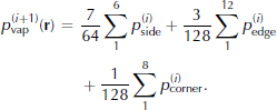
case 2 If at least one neighbour belongs to the ice, digitization Equation (8) is used. Hence:
In both cases, when at least one neighbouring voxel of v(r) does not belong to the image file, it is not taken into account in the ![]() estimation. In other words, the digitization is restricted to the available data by computing the weighted mean of
estimation. In other words, the digitization is restricted to the available data by computing the weighted mean of ![]() on the inner voxels only (see section 2.4).
on the inner voxels only (see section 2.4).
6. Procedure (5) is iterated until the field of p vap(r) converges.
The gradient ∇p (r) is then evaluated on the closest non-adjacent layer to S using Prewitt’s digitization of the gradient operator (Reference Prewitt, Lipkin and RosenfeldPrewitt, 1970). The resulting growth rate R is then computed using Equations (6) and (7). If time-lapse evolution of snow microstructure was required, the next step of the simulation would consist of modifying the grain surface S according to the field of surface fluxes. The computation of p(r) and R(r ∈ S+εn) from the newly obtained surface would result, if repeated, in a morphological iterative process that would provide the microstructure evolution of snow with time.
3. Preliminary Results and Outlook
Vapour field and growth rate computations were first checked qualitatively on two spheres of different radii. The test showed matter accretion (positive flux) on the large sphere, close to the small one, unlike the result with a reaction model (Fig. 1). This is the sort of difference we can look for between further simulations of metamorphism using both the reaction and diffusion processes. For both models, p amb was initialized as the saturation pressure, corresponding to

Fig. 1. (a) Qualitative map of the mean curvature κ of a system of two neighbouring spheres of different radii; (b) growth rate R in the reaction case (spheres do not ‘see’ one another); and (c) R in the diffusion-limited case (vapour transfer is favoured between close grains).
The computations were then applied to tomographic 3-D data (Reference BrzoskaBrzoska and others, 1999) acquired from the European Synchrotron Radiation Facility (ESRF, Grenoble, France). The snow images presented in this paper refer to a snow sample obtained at −2 ˚ C after a metamorphosing time of 12 days (Reference Flin, Brzoska, Lesaffre, Coléou and PieritzFlin and others, 2004). Figure 2 depicts a 2-D slice of the computed vapour field.
Fig. 2. A 2-D slice of the computed vapour-pressure map in the diffusion-limited case. The snow image presented here was obtained after metamorphosing during 12 days under isothermal conditions. Image edges are 300 voxels (∼3 mm) wide.
In order to check the representativeness of the computed vapour field, the mean values of vapour pressure were computed in cubic neighbourhoods growing from the centre of the 3-D image. The vapour pressure averages vs the size of the computing volumes are plotted in Figure 3. The same process has been applied to two other samples: a recent snow sample obtained after 2 days of isothermal metamorphism (Reference Flin, Brzoska, Lesaffre, Coléou and PieritzFlin and others, 2004) and a slightly faceted sample taken after 3 weeks of TG metamorphism (TG = 3 Km − 1, average temperature ∼–3 ˚ C) (Reference Flin, Brzoska, Pieritz, Lesaffre, Coléou, Furukawa and KuhsFlin and others, 2007). From Figure 3, it appears that the REV for vapour pressure significantly depends on the snow microstructure. The REV for the 12 day old sample (A) can be approximated as the volume of a cube of 2.5–3.0mm in dimension. However, the REV for the recent snow sample (B) (TG sample (C)) seems much larger (smaller).
Fig. 3. Vapour-pressure REV estimations for different samples.
Figure 4 shows the growth rate results of both reaction and diffusion-limited models for the same 12 day old sample. (The result for the reaction model is scaled by the effective reaction coefficient α that has not yet been precisely assessed from the experimental data.) One can see a sharper transition between positive and negative growth rates in the diffusion process, which is consistent with results on spheres. Local transport is favoured, then enhances the contrast of the crossover between regions of positive and negative R. It will be interesting to check regions where two (convex) grains of different average curvature are close to each other, where the above situation of two spheres is expected.
Fig. 4. (a)Map of the growth rate Rin the reaction case scaled by the effective reaction coefficient α; and (b) map of R in the diffusion-limited case. Image edges are 300 voxels (∼3 mm) wide. Growth rates are expressed in 10 − 10 ms − 1.
The most interesting comparisons remain to be made between numerically metamorphosed results of both models from the same input snow data. One can reasonably expect visible changes in curvature histograms between these two simulations, and therefore a comparison with the experimental histogram may answer the difficult question of whether the diffusion or the reaction mechanism is dominant for the given experimental conditions. The only requirement is that models should be run on data files that are representative of samples larger than the REV of vapour transfer. Further developments will have to deal with the intrinsic slowness of iterative schemes. It will first be necessary to replace the Jacobi method with a more efficient scheme. For example, over-relaxation methods (Reference PatankarPatankar, 1980) could be used to implement the model on nested cubic grids, adopting the low-resolution result as a guess for the final high-resolution run.
Acknowledgements
We thank J.B. Johnson and an anonymous reviewer for constructive comments. F. Flin is grateful to Y. Furukawa for his welcome at the Institute of Low Temperature Science as a guest researcher.

