1. Introduction
The surface roughness of the snowpack controls the transfer of wind energy to the surface (Reference Fassnacht, Williams and CorraoFassnacht and others, 2009a, Reference Fassnacht, Stednick, Deems and Corraob). It is also an important factor for the scattering of light and thereby related to the surface albedo (Reference WarrenWarren, 1982;Reference Leroux and FilyLeroux and Fily, 1998;Reference Warren, Brandt and HintonWarren and others, 1998; Reference Mishchenko, Dlugach, Yanovitskij and ZakharovaMishchenko and others, 1999; Reference Zhuravleva and KokhanovskyZhuravleva and Kokhanovsky, 2011), which is one of the essential climate variables (ECV) defined in the Implementation Plan for the Global Observing System for Climate in support of the United Nations Framework Convention on Climate Change (UNFCCC; http://unfccc.int/2860.php). In addition, the backscattering in microwaves is sensitive to surface roughness. The rough ness information needed is related to the microwave wavelength (Reference ManninenManninen, 2003). The length of the profile should cover at least ten times the wavelength, and the pixel size should be smaller than ~0.1 times the wavelength. For example, to describe roughness relevant for C-band the profile should be at least 50 cm long and the pixel size should be <5 mm. Our system fulfils both requirements.
Snow surface roughness depends on the complete history of the snowpack and the prevailing status starting from the precipitation event. The changing weather conditions (temperature, wind and humidity) cause metamorphism until the snow melts completely. In addition, every snowfall after the formation of the first snow layer causes step- function-like changes in the surface structure.
There are dozens of commonly used surface-roughness- describing parameters, and the proper choice depends on the application (Reference Dong, Sullivan and StoutDong and others, 1992, Reference Dong, Sullivan and Stout1993, Reference Dong, Sullivan and Stout1994a, Reference Dong, Sullivan and Stoutb). In remote-sensing applications the root-mean-square (rms) height and correlation length are typically used, but if they are treated as scale-invariant parameters they do not characterize natural surfaces well (Reference Keller, Crownover and ChenKeller and others, 1987; Reference ChurchChurch, 1988;Reference ManninenManninen, 1997, Reference Manninen2003). Therefore, multiscale surface roughness characterization methods more or less related to fractals and fractional Brownian motion (fBm) have been developed (Reference Davidson, Le Toan, Mattia, Satalino, Manninen and BorgeaudDavidson and others, 2000;Reference ManninenManninen, 2003). The multiscale nature of snow surface roughness was recently demonstrated by Reference Fassnacht, Williams and CorraoFassnacht and others (2009a,Reference Fassnacht, Stednick, Deems and Corraob).
In order to properly characterize the temporal and spatial variation of the snow surface, one has to be able to gather a large number of profiles in variable land-cover types. Therefore the measurement system should be robust and lightweight and preferably one should be able to work the whole day without needing to recharge batteries. Taking photographs of the snow surface against a dark background plate fulfils these requirements. In addition, it is easy to use this technique in dense forests and difficult terrain, where many other measurements are difficult to carry out. Reference Fassnacht, Williams and CorraoFassnacht and others (2009a,Reference Fassnacht, Stednick, Deems and Corraob) demonstrated the use of digital images of the snow surface against a board partially buried in the snowpack. Their image analysis was interactive and the calibration was made by comparison with manual measurements. Reference Elder, Cline, Liston and ArmstrongElder and others (2009) used a similar technique for snow surface profiling. The only drawback so far has been the time-consuming image analysis and calibration afterwards. Here we present an advanced version of this kind of profiling technique, which is based on automatic image analysis and calibration including removal of barrel distortion of the images. This study presents a fully automatic procedure for analysing the photographs and calibrating the profiles in millimetres. Even if manual interaction is needed in exceptionally difficult cases, the snow profile and control points are always automatically determined, so the result is operator-independent.
2. Measurement System
The measurement system consists of a background board and a digital camera. The middle part of the board (100 cm × 40 cm) is black (Fig. 1). The surrounding edges are covered by three rows of black-and-white squares with dimensions of 1, 5 and 10 mm. The width of the scale bands is 10 mm for all three scales. The board is made of a 3 mm thick white I-bond aluminium layer plate, whose surface layers are made of thin aluminium while the inner parts are made of polythene. The plate is covered with black matte tape. The scales at the edges are engraved on a 0.8 mm thick laser engraving plate, which is attached to the board using thin two-sided tape. The weight of the board is 1.9 kg.
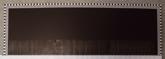
Fig. 1. The plate used as background and scale for the snow surface roughness measurements, here shown in calibration measurements using a print of scaled tooth pattern.
The photographs were taken with a Canon PowerShot G10 digital pocket camera. This was chosen because a pocket camera is practical in field measurements due to its light weight and ease of handling. The camera has a sensor of 4416 × 3312 pixels and a zoom lens from 6.1 to 30.5 mm having an optical image stabilizer. The range of focal lengths used varied between 6.1 and 25 mm, which yield angular fields of view from 63.8° × 47.1° (vertical) to 17.3° × 12.1°, respectively. The longer focal lengths were used when it was not possible to get closer to the board (e.g. when the snow surface needed to be kept intact for later use). The use of a wider field of view produces more barrel distortion, but is generally easier to handle in the field. The camera can produce both JPG and raw image formats. JPG format was used, as the file size is much smaller, it is a well-supported format, and the extra bit-depth (12 bits vs 8 bits per pixel) or linearity of the image data were not needed in this application.
Snow measurements are carried out by carefully inserting the plate partially into the snowpack and taking a photo graph roughly perpendicularly to the background board surface, so that a picture containing the snow/board inter face is obtained. One photograph is sufficient to retrieve the surface profile, but, in field measurements, taking redundant images is recommended to increase the possibility of fully automatic analysis for each profile;varying illumination conditions and (possible) snowflakes in the plate area cause a challenge for completely automatic image analysis.
The measurement system was constructed for the Snow Reflectance Transition Experiment (SNORTEX) campaign in Sodankyla, northern Finland (Reference RoujeanRoujean and others, 2010), and the majority of the demonstration images presented were taken during that campaign. The analysis method was first adapted to that dataset, but slight modifications were needed later to guarantee automatic analysis for the Radiation, Snow Characteristics and Albedo at Summit (RASCALS) campaign at the Greenland summit (Reference Riihelä, Lahtinen and HakalaRiihela and others, 2011) and for method consistency measurements carried out in Kirkkonummi, Finland, by the Finnish Geodetic Institute.
3. Analysis Method
The snow surface is retrieved from the blue channel of the red, green, blue (RGB) image as a threshold between light and dark pixels. In practice, automatic snow surface recognition is much more difficult due to problems related to real-world conditions. The following main problems are identified:
-
varying contrast between images due to varying illumi nation conditions
-
varying contrast within an image (e.g. due to specular reflection of sunlight;shadows on the snow surface;flash light; partial wetness of the board surface)
-
litter (such as needles) on the snow surface
-
snowflakes in the area of the plate due to a snowfall during measurements
-
varying orientation and size of the visible part of the background board
The main logic for finding the snow surface is shown in Figure 2. Full details of the method are not given here, as the code is 25 pages long in the notebook form of Wolfram Mathematica 8.0.1.0. The orientation and fraction of the plate visible in the image can vary over a wide range, because the board will sink deep down in a fluffy snowpack, whereas in the hardest snowpacks one has to saw a slot, before the board can be inserted into the snow. The starting point for the analysis is to find the location of the background board in the image. The board is located on the basis of the image intensity distribution characteristics of the lower half of the image. The upper half is not used, because its intensity values may vary in a wide range depending on whether the background is dominated by the sky or trees.
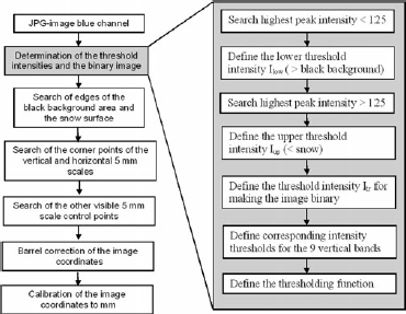
Fig. 2. Logistic of the search of the snow surface pixels and calibration to millimetres.
The highest peak of the intensity distribution smaller than or equal to 125 is sought first. Starting from intensity matching the peak frequency, the intensity values for which the frequency has dropped to 10% of the peak value are determined on either side of the peak. The smaller intensity value is I 1 and the higher I 2. The lower threshold intensity is then defined as Ilow = I2 + (I2-11)/2. The black area of the plate should mostly have intensity values smaller than I low. Likewise the highest peak larger than 125 is sought. The lower and higher intensity values matching the 10% height of this peak are I3 and I4. The upper threshold intensity is chosen to be Iup= I3 + (I4-13)/2. The snow intensities should mostly be higher than Iup. The threshold intensity Itr used to make a binary version of the image is then the average of Ilow and Iup, so that, in the binary image, intensities lower than Itr are -1 and intensities higher than Itr are 1 (and intensities equal to Itr are 0). Before starting the analysis the image is cropped in order to speed up processing and to decrease the effect of the image background. This step is, however, not absolutely necessary and its details are not described here.
Due to varying illumination and specular reflection of sunlight, the intensity of the black part of the plate is not constant. Therefore the intensity distribution of the quarter of the image just below the middle is analysed in nine vertical bands situated from 14% up to 82% of the image width (Fig. 3). The larger width of one band is only due to historical reasons. The original number of bands was fewer than nine, but it was increased when more problematic images ap peared. Distribution analysis is a relatively slow operation, hence only the number of bands really needed is used, regardless of the fact that one band has double width. The threshold intensity is determined for each band i as I tri = (4I lowi/ + I upi)/5. Here I lowi and I upi are determined for each band in the same way as for the whole image. A second-order polynomial is then fitted to the values Itri as a function of the band centre horizontal coordinate. Additional fine tuning not described here is applied to the threshold function, which is then used in the following process instead of a constant intensity threshold for the whole image. The edges of the visible part of the black area of the background board are then sought. Starting from the black background area, the right, left, top and bottom edges are derived using intensity thresholds based on the threshold polynomial (Fig. 3). For the vertical edges the starting point is pixel columns one-third and two-thirds of the image width. For the horizontal edges, the starting point is the middle height row of the image. The intersections of the top, bottom, left and right edges found this way are used to discard the tail parts of these edges, so that an essentially rectangular point set is left. The detected edge coordinates are then iterated using distribution analysis so that in the end second-order polynomial fits to the point sets of each edge produce high values for the coefficients of determination for the regression (Fig. 4).
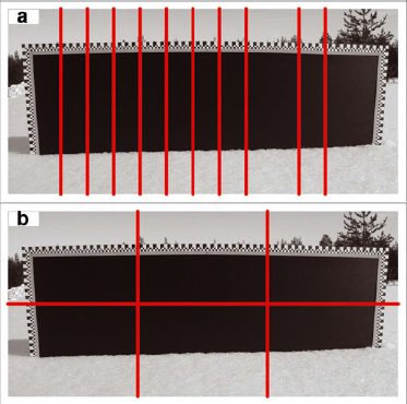
Fig. 3. (a) Location of the nine vertical bands used to determine the intensity distribution. (b) Location of the vertical and horizontal lines used as starting points for searching the left, right and top edges of the black background and the snow surface.
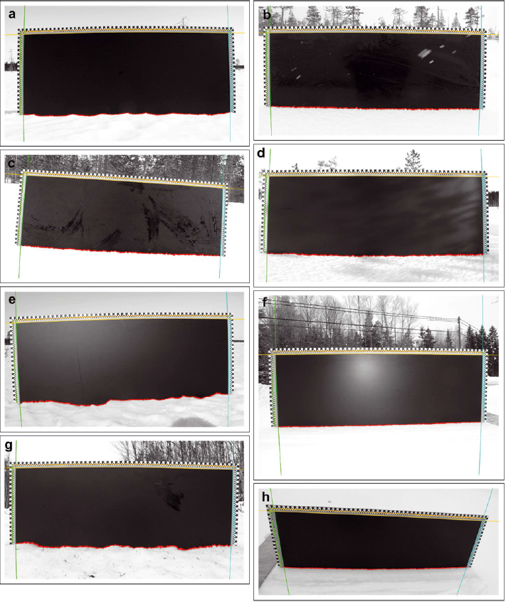
Fig. 4. Examples of automatic detection of the edges of the black background area. (a) is an example of easy analysis. The other panels demonstrate fully automatically analysed, but more challenging, cases of (b) snowfall (c) traces of wiping the black background dry, (d) uneven shading, (e) reflected sunlight, (f) reflected flash light, (g) needles on the snow surface and (h) a tilted plate. The detected edges of the black background are indicated with continuous curves. All the automatically detected control points of the 5mm scale used for calibration of the images are also shown.
The snow surface is normally searched starting from the middle part of the black background plate in order to avoid problems of litter or shadows on the snow surface. In the event of snowfall, it is assumed that the snow surface is pure and without shadows. The snow profile is then searched starting from the lower edge of the image, detecting the threshold of pixel values when moving from the snow pixels to the black area of the background board.
The intersections of the polynomials fitted to the left and right edges and the upper edge of the black background area are used as starting points in searching for the corner points of the vertical and horizontal 5 mm scales surrounding the plate. Knowledge of the chequer pattern of the plate in the corner area is used as the basis in this process, which is carried out using the binary version of the image. Examples of detected corner points are shown in Figure 5. The rest of the control points to be detected are cross sections, which are corner points of four 5 mm squares. The shapes of the polynomials fitted to the left, right and upper edges of the black area are used as directional guidance in the search of the control points. Detection of the upper edge points is facilitated by the knowledge that there are exactly 205 points to be detected on top of the corner points. When the corners are found, the curve between them contains 203 control points almost evenly spaced, because the viewing direction is in measurement configuration almost perpendicular to the plate surface. The positions of those control points are found iteratively starting from the rough evenly spaced positions. Changing of the black and white areas from right to left and from above to below the guidance curves is checked. The number of the visible left and right control points varies, but it is clear that no control points can be detected from below the snow surface, so that the left and right ends of the snow surface profile are used as limiting factors. The exact location of all control points is determined iteratively to achieve the best match to the black-and-white structure. Examples of detected control points are shown in Figure 4.
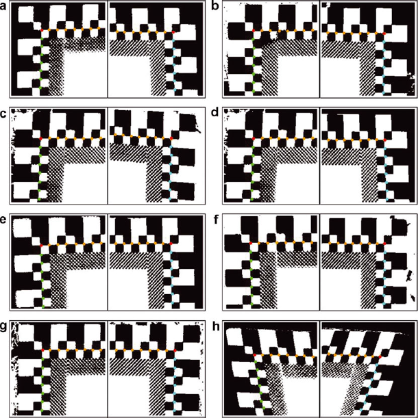
Fig. 5. An example of automatic detection of the corner points (red) of the 5 mm scale used to calibrate the images. The other control points fitting in the image are shown in other colours. The background image is the thresholded negative of the original image, Figure 4a-h.
The wide-angle optics used here caused barrel distortion to the image coordinates. This effect had to be removed from the detected snow-surface and control-point image coordin ates before calibrating them to mm values. The coordinates of an ideal undistorted image fu(x, y) and the distorted image ![]() are related by (Reference Farid and PopescuFarid and Popescu, 2001)
are related by (Reference Farid and PopescuFarid and Popescu, 2001)
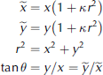
where r is the radius of the point in the undistorted image, θ is the azimuth angle of the point and k is either negative (convex distortion) or positive (concave distortion). Here it is assumed that the lens is spherically symmetrical. In the configuration used in this study, k is always negative. The value for k is determined so that it minimizes the difference of the true control point coordinates and their estimates derived using Eqn (1). The undistorted coordinate values of the snow surface profile are then calculated applying this optimal value of k and the image coordinates of the detected snow surface points to Eqn (1). The lens distortion parameter is derived for every image separately in order to achieve maximal accuracy. The mean value for k was -0.018, and the standard deviation was 22% of the mean value.
If fixed optics were used instead of a zoom lens system, the camera could be calibrated in laboratory conditions and the same barrel distortion would apply to all images. However, taking photographs in forest often restricts the possible viewing angle so that without zoom it would not always be possible to take a photo so that the whole plate is visible in the image.
Coordinates can easily be converted from one plane to another using the transformation introduced by Reference Haggren, Manninen, Peralainen, Pesonen, Pontinen and RantasuoHaggren and others (1995). Thus the coordinates in the image plane (x, y) are related to the coordinates with respect to the background board scales (xmm , ymm ) via
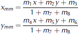
where parameters mi (i = 1-8), can be determined using four control points, for which both the image and board coordinates are known. However, the imaging configuration is not ideal for coordinate transformations since there are no control points below the detected snow profile. Therefore we use all detected control points as the basis of the coordinate transformation into mm values and determine the m,--parameter values by regression. After calibration into millimetres, the profiles may be inclined with respect to the horizontal axes depending on the orientation of the back ground plate in the snowpack (Fig. 6). The profiles are then rectified with linear regression so that the average slope is zero. In addition, the profiles are corrected with the residual calibration parabola fitted to the horizontal axes (Section 4) to obtain the final profiles (Fig. 7).
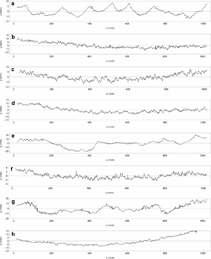
Fig. 6. Examples of automatically detected profiles corresponding to the images, Figure 4a–h.
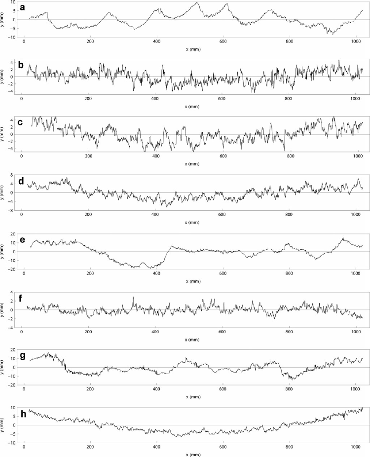
Fig. 7. Examples of automatically detected and rectified profiles corresponding to the images in Figure 4. The calibration paraboloid has been subtracted from the profiles.
The software developed also produces a copy of the original image, where the profile and control points are merged. The copy can also be used for quality-check purposes. The main point of the visual inspection is to check that all control points are found and located correctly. Detection of the vertical control points is especially demanding, as it is not possible to know in advance how many of them will be visible in the image. Correct snow profile detection does not normally cause difficulties.
4. Calibration
The vertical accuracy of the coordinates was first tested by taking a photo of a straight horizontal paper edge and analysing it with the same automatic method as used for the snow profiles. The average absolute deviation of the meas ured height from zero was 0.93 mm with a distinct parabola shape (y =0.0000144 ∞ 2?0.01479x + 2.609;R2 = 0.99). When the coordinates were corrected with respect to the fitted parabola, the remaining average absolute deviation from zero height was 0.07 mm. The parabola is believed to be due to the scale being projected slightly (1 mm) above the plane of the black background. Partly it may also be residual error from the barrel distortion correction.
The horizontal and vertical accuracy was studied more thoroughly by taking photos of a rack-tooth pattern with dimensions of 5 mm × 5 mm from different heights and angles (Fig. 1; Appendix 1). About three images were taken for each setting, and one image per setting was included in the dataset of 50 images used in the analysis. In addition, a smaller dataset of 30 images, which included only the cases with realistic measurement settings, was chosen (Appen dixes 1 and 2). For instance, images with (1) >1.5 m distance from the plate, (2) extreme measuring angles or (3) extreme positioning of the rack-tooth patterned profile on the plate were excluded.
In general, the measured profiles are not located at the same part of the image; hence the residual barrel distortion is individual. The varying positioning of the rack-tooth pattern (Appendix 1) was used to test this. It turned out that the second-order coefficient of the residual parabola was correlated with the parameter k of Eqn (1) and the coordinates of the starting and end points of the profile (R 2 = 0.61 images representing viewing variation in typical range). A simple second-order rational polynomial of these three variables was then constructed and used for residual barrel correction. The parameter values of the polynomial were derived using both (1) all images and (2) the subset of typical viewing configurations. For each measurement, statistical parameters were derived for three alternatives: (1) no residual barrel distortion correction, uc, (2) general residual barrel distortion correction, gc, (function param eters identical for all profiles) and (3) optimized residual barrel distortion correction, oc (function parameters opti mized separately for each image).
The median and 0.9 quantile of the heights of the rack teeth were calculated for each profile using the distance between the upper and lower rack-tooth envelope surfaces (Appendix 2). The 0.1 quantile was not relevant since it was mostly dominated by points midway between the envelope surfaces. The distances between successive ascending-edge horizontal coordinates of the rack teeth and the distances between successive descending-edge horizontal coordinates of the rack teeth were also calculated. From these values median, 0.1 quantile and 0.9 quantile for each profile were derived. Finally the average, median, 0.1 quantile and 0.9 quantile values of the individual profile statistical parameters were calculated (Table 1). The summary values of the three alternatives are similar and, curiously, the optimized version is not always the best. In addition, corresponding summary statistics were calculated for the smaller dataset that included only the cases with realistic measurement settings (Appendixes 1 and 2). The median and average values of the subset were about the same as for the total, but the 80% variation range was markedly better for the subset than for the whole dataset.
Table 1. Statistics for the profiled rack-tooth dimensions. The three different statistical parameter values correspond to Appendix 2. The values are shown for the whole dataset (All) and a subset corresponding to cases with realistic measurement settings (Selection). For the racktooth heights, median and 0.9 quantile were calculated. For the rack-tooth widths, median 0.9 and 0.1 quantile values were calculated (see Appendix 2 for values of individual profiles). For each of these, average, median, 0.1 quantile and 0.9 quantile were calculated. (See Appendix 1 for the original images used for the figures)
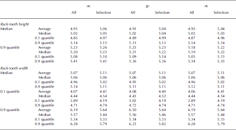
On the basis of the rack-tooth pattern analysis, the estimated overall horizontal accuracy of the measurement system is on average 0.1 mm, and in 80% of cases the error varies in a range smaller than ±0.6mm. Likewise the estimated overall vertical accuracy is on average 0.04mm, and in 80% of cases the error varies in a range smaller than ±0.2 mm.
With rack-tooth surface height difference measurements, the method had clear problems with images 6252, 6329, 6332, 6378, 6381 and 6392 (Appendixes 1 and 2). These are all cases that do not describe realistic field measurement settings and were not included in the realistic subset. For image 6392 the problems are probably caused by the fact that the left-side scale is only visible for such a short distance. This complicates the fitting of the polynomial on the side of the plate, thus causing error in the results. For images 6378 and 6381 the vertical scales on both sides are short.
For image 6252 the failure has to do with the focus of the image or some other factor related to this particular image. For another image of this particular setting (6251), the corresponding values for the median of the height difference between rack-tooth surfaces are 5.0544(uc), 5.028(gc) and 5.0291(oc). Values for the horizontal length of the rack-tooth surfaces in the 0.1 quantile are 2.43 (uc), 2.42(gc) and 2.43(oc), and in the 0.9 quantile are 7.61(uc), 7.62(gc) and 7.61(oc). These values are more in line with the rest of the measurements.
As there was no suitable tripod/camera support available, the images were taken hand-held, causing some random blurring to the images. Images 6329 and 6332 were taken from 2 m height and the resolution was modest. The result was that some of the slightly blurred vertical edges of the rack teeth were not detected or were 'detected twice' (Appendix 2). For the horizontal accuracy measures of the rack-tooth pattern, the images that stand out in addition to those already analysed in the vertical accuracy values are 6271 and 6283. In the 0.9 quantile, values of the horizontal length of the rack-tooth surfaces for image 6283 were close to 10 mm. This error is likely to be caused by the angle of photography and camera, and the position of the plate close to the edge of the image, as the barrel distortion is largest at the edge parts of the images.
The repeatability of the method was tested by comparing the three different images taken from one measurement setting (Appendix 3). Twenty-one settings had three success ful images of them and thus were included in the analysis. The root-mean-square (rms) height variation was calculated for each image using a moving window of varying size. The average rms values corresponding to each window size were then calculated. The wider the window is, the fewer separate rms values are available for the average. Therefore the average rms values representing the longest distances have a high random variation, so it is better not to use the values obtained for longer distances than ~60% of the whole profile (Reference Manninen, Rantasuo, Le Toan, Davidson, Mattia and BorgeaudManninen and others, 1998). The calculated statistics include the mean value, standard deviation, the difference between the highest and lowest rms value and the percentage of this variation of the mean value for every triplet of rms values. In addition, the mean value and the standard deviation of the triplets' statistics are shown for each parameter. The results show that the standard deviation of the rms values per measurement is <0.02 mm. The variation of the rms height measurement is typically <1% of the mean value. The measurements that have poor figures are 7, 11, 13 and 14. These measurements typically have one image in the set that has values noticeably different from the other two images. Many of these also had problems defining the rack- tooth pattern dimensions correctly, indicating that these settings include an image that is out of focus.
The effect of the temperature variation on the dimensions of the scale was estimated to be <0.1% for a typical measurement temperature range.
5. Results
So far, 1190 profiles have been analysed using the presented method. More than 99% of them passed the automatic processing. Examples are shown in Figure 7. The snow surface is mostly off from the background plane. Therefore all profiles are corrected for the residual parabola (see Section 4), although the effect was normally negligible (of the order of 0.01 mm) at the mean height of the rack teeth. The rms height variation with distance is shown in Figure 8 for the studied profiles. Clearly the visual impression of roughness is confirmed by the rms height values. The variation of the rms height with distance is in line with the results of Reference Fassnacht, Williams and CorraoFassnacht and others (2009a,Reference Fassnacht, Stednick, Deems and Corraob) Detected reasons for failure of automatic analysis are (1) blurred or out-of focus image, (2) a very dark object at the front of the image, snowflakes at the corners of the black background, snowflakes on the scale part of the image or (5) extremely poor contrast of the image intensity, i.e. the 1 mm scale squares cannot be thresholded to produce a black-and-white chequer pattern. But even in a case when manual intervention was needed to detect the board or adjust the intensity thresholds, the actual snow surface profile and control point determination was always carried out fully automatically.
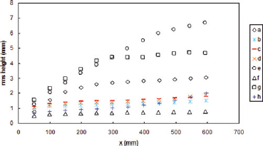
Fig. 8. The rms height variation of the measured profiles as a function of distance.
The repeatability of the measurement system was tested by taking three different photos of the same plate pos itioning. Because the surface was the same, the end result should also be equal, although the viewing configuration of the manually held camera certainly varied between the triplets so that neither the inclination nor the azimuth direction of the camera was constant. Illumination and weather conditions did not usually change so rapidly that the same snow surface could be analysed in different conditions. Results of such triplet profiles are shown in Figure 9. The standard deviation of the profiles varied in the range 4.7?4.8 mm, and the corresponding relative value was within 0.98?1.01% of the mean value. This example corresponds to a normal viewing configuration variation.
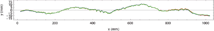
Fig. 9. Three different profiles (red, blue and green) of the same surface analysed automatically.
To test the effect of varying viewing configuration in a wider range in field conditions, a set of nine images was taken (Fig. 10). The viewing angle was varied in a wider range than in normal measurements, and the contrast of the image was varied as much as was possible in the prevailing illumination conditions. Finally, some shoots of spruce were added at the front area of the image to test their effect on the analysis. For these nine images, the mean rms height value corresponding to 600 mm distance was 2.42 mm, with a standard deviation of 2.7% of the mean value. The largest deviation from the mean value came from images c, d and h. The first two images represented cases in which the resolution was clearly poorer due to the choice of the zoom position. The last case corresponded to an exceptionally large azimuth viewing angle, which caused marked reso lution deterioration at the left edge of the image. When these three images were excluded, the mean rms height value was 2.45 mm, with a standard deviation of 1.2%. It is natural that reducing resolution decreased the rms height, because more details were smeared out.
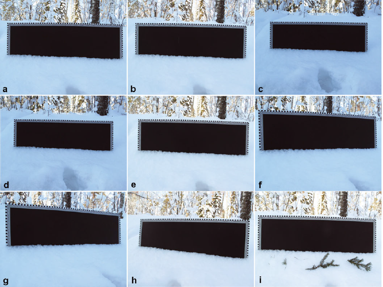
Fig. 10. Nine different viewing configurations for the same surface profile.
6. Discussion
The zoom lens was chosen to enable photos to be taken even in relatively dense forests, where it is not possible to use long distance between the camera and the plate. Therefore the lens parameter needed for the barrel distortion correction has to be determined for every image separately. Here it was assumed that the distortion is spherically symmetric, but this is not necessarily the case. Thus it is possible that some of the residual distortion is due to this assumption. One could have allowed different distortion parameter values in the vertical and horizontal directions, but sometimes the visible parts of the vertical edges were so short that it was not considered wise to use them to determine separate vertical distortion parameters.
Because the plate is planned to be portable in various kinds of terrain and land cover, the width is limited to 1 m. Hence, the current plate is suited to surface roughness measurements corresponding to the wavelengths of radars in C- and X-band. The height variation that can be measured using the plate is ~40 cm, which was sufficient in all studied cases. However, if the snow cover has large-scale roughness features so sparsely distributed that they do not necessarily appear within the width of the plate, the large-scale roughness will not be properly characterized with this measurement technique. This kind of roughness can typic ally be found on lake ice, where the wind may accumulate the snow in sparse scale-shaped bumps.
For surface albedo, all roughness scales from the grain size upwards to larger topographical features are mean ingful. This measurement technique is suitable for character izing the smaller edge of the roughness scale, but the larger features need other instruments unless the surface is so clearly fractal that the 1 m long profiles can be used for upscaling the roughness values (Reference ManninenManninen, 2003).
Although the analysis method worked well enough to provide automatic results in most cases, an even more robust algorithm could be generated if the plate were slightly improved. In difficult illumination and weather conditions, finding the edges of the black background caused dif ficulties. Detection of the black area would be easier if it were surrounded by a few continuous 5 mm wide white and black bands instead of the innermost 1 mm chequerboard band. When the illumination is low, the contrast between the black and white squares is relatively poor and causes difficulties in picking up the control points. Using highly reflecting paint for the white squares might improve this. One side of the plate could be black and white, as now, for bright daylight work, and on the other side the white could be replaced by a highly reflective paint for moonlight and twilight work.
Although the software in its current form cannot be readily distributed (as it is tailored to the plate used), we invite readers interested in the code to contact us. We will be happy to cooperate in making the code generally available. If an improved version of the plate is made as suggested above, the code could also be markedly simplified.
7. Conclusions
The developed analysis method for snow surface roughness measurements works autonomously in 99% of cases, so the accuracy is operator-independent. The system requires only a photo and information as to whether it was taken during a snowfall or not. The vertical average accuracy is 0.04mm and the horizontal average accuracy 0.1 mm.
Typical causes for failure of the fully automatic analysis are: (1) insufficient contrast of the image, (2) snowflakes covering the control point scale or upper corners of the black background and (3) fuzzy photo. In order to maximize quality, one should pay attention to the resolution and available light in field conditions. It is a good option to take photos with and without flash, when the illumination is low. The viewing angle is normally perpendicular enough to not reduce the quality of the results.
Acknowledgements
This work was financially supported by EUMETSAT through the project Satellite Application Facility in Climate Moni toring and the project Satellite Applications on Support to Operational Hydrology and Water Management, and by the Finnish Academy of Sciences through the project 'New techniques in active remote sensing: hyper spectral laser in environmental change detection' (255534).
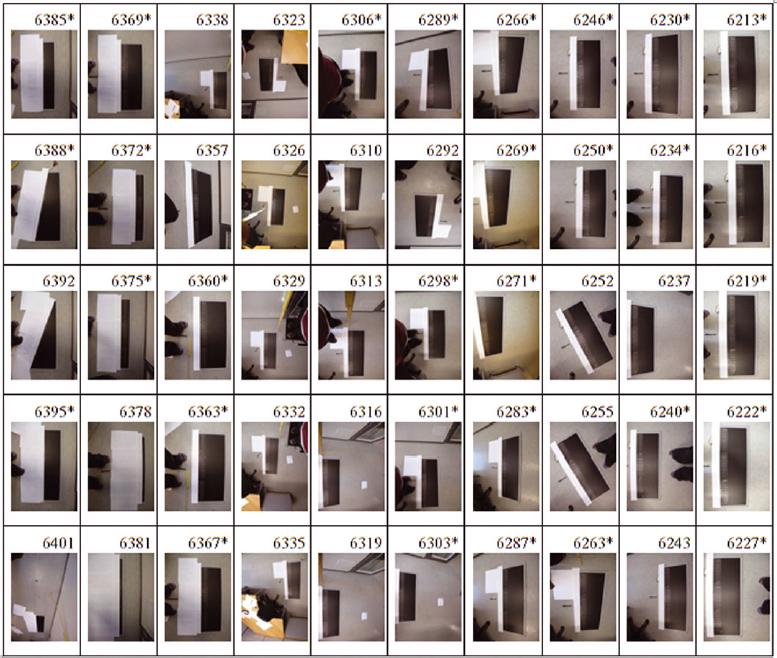
Appendix 1
Images used in the rack-tooth pattern profile measurements. The images marked with * are also used in the subselection of realistic measurement cases (see Table 1).
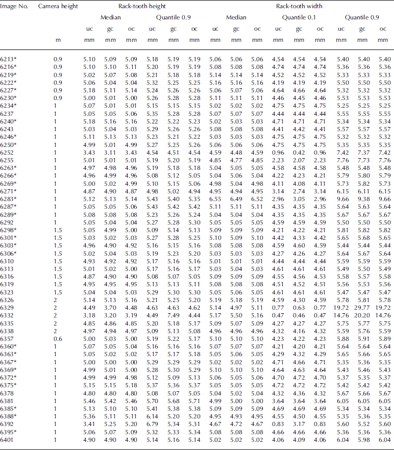
Appendix 2
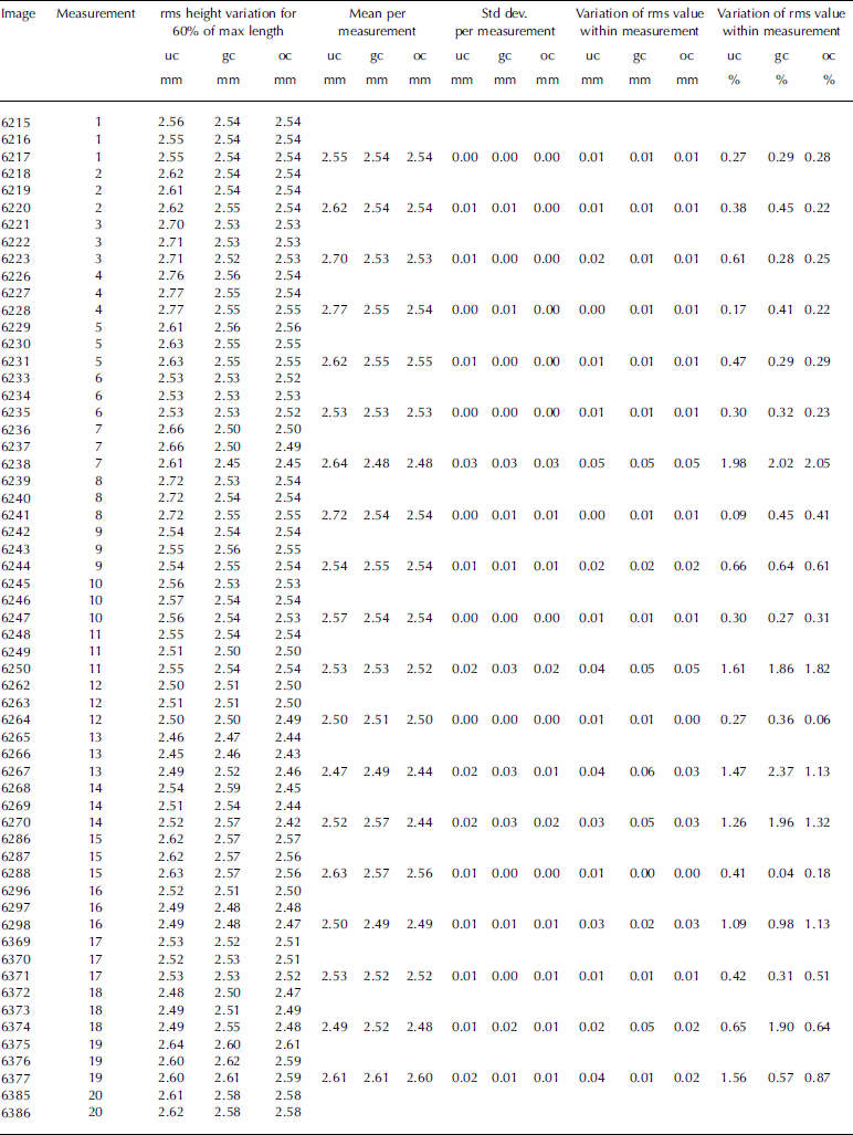
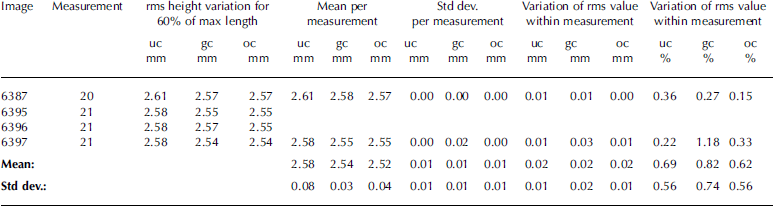
Statistics for the height and width of individual rack-tooth pattern profiles. Images marked with * in the Image No. column were also used in the subselection of realistic measuring cases (Table 1). Three different sets of statistical parameters were used: (1) without extra correction for the residual curvature (uc), (2) with general correction for the residual curvature (gc) and (3) with correction of the residual curvature optimized separately for each image (oc). The median and 0.9 quantile of the rack-tooth height were calculated for each profile for the distances between the two adjoining rack-tooth surfaces. For the rack-tooth width the median, 0.1 quantile and 0.9 quantile are shown here. Both the ascending and descending edge differences were included in the statistics. Each image represents a separate measurement. For the images see Appendix 1.
Appendix 3
The statistical parameters of the three image sets of individual rack-tooth pattern measurement settings.