


Introduction
Snow is an important component of the cryosphere. More than one sixth of the world's population rely on water from snowmelt for drinking water, irrigation and hydroelectricity (Barnett and others, Reference Barnett, Adam and Lettenmaier2005). Flooding caused by rapid snowmelt is a contributor to overall flood risk. Snow cover can also reduce flood risk because precipitation which falls as snow can be retained in the snowpack to be released to rivers slowly as snowmelts. Snow can also be a major hazard. It causes delays to ground and air transport, increases the number of injuries in accidents and can damage crops and livestock. Avalanches in mountain areas are a significant risk to property, infrastructure and life (Mitterer and others, Reference Mitterer, Heilig, Schweizer and Eisen2011).
To predict risks and manage resources, models are used widely to forecast snow accumulation and melting. Models used operationally across the globe vary from simple accumulation and melt models based on air temperature and precipitation, to complex multilayer physically based models, such as those described in Lehning (Reference Lehning2009); Magnusson and others (Reference Magnusson2015) and Dong (Reference Dong2018). Snow hydrological observations are required to drive and verify model simulations, but limitations on geographical extent, resolution and the invasive nature of some observations introduce uncertainties into model predictions (Wever and others, Reference Wever, Fierz, Mitterer, Hirashima and Lehning2014; Largeron and others, Reference Largeron2020). These uncertainties are compounded by the complex behaviour of snow hydrology systems (Essery and Etchevers, Reference Essery and Etchevers2004; Essery and others, Reference Essery, Morin, Lejeune and B Ménard2013; Magnusson and others, Reference Magnusson2015). Satellite data are used widely to assimilate into global land surface models, but despite recent advances it is not possible to measure internal water fluxes and assimilate into and verify high-resolution multilayer models (Tsai and others, Reference Tsai, Dietz, Oppelt and Kuenzer2019; Largeron and others, Reference Largeron2020). Manual monitoring of snow variables such as using snow pits provides high-resolution data at discrete locations (Kinar and Pomeroy, Reference Kinar and Pomeroy2015), but data coverage is sparse, especially in high altitude and polar regions. Automatic monitoring of snow provides greater geographical coverage in remote locations. Liquid water in snow is an important control on many of the risks noted above, especially snowmelt runoff and avalanche risk. Measuring liquid water content using current methods has significant limitations.
Volumetric water content (θw) can be measured using calorimetric methods. These measure how much heat is required to melt a known volume and mass of snow, and calculate θw from this. This method is not suited to automatic operation and, due to its destructive nature, is not suitable for in situ monitoring (Kinar and Pomeroy, Reference Kinar and Pomeroy2015). Electrical methods, which exploit differences in the dielectric permittivity between liquid water, air and ice, offer more promise for automatic sampling and in situ monitoring. Examples of these include the Denoth Meter, Finnish Snow Fork and Snowpack Analyzer which work using similar principles (Tiuri and others, Reference Tiuri, Sihvola, Nyfors and Hallikaiken1984; Denoth, Reference Denoth1994), and capacitance methods (Avanzi and others, Reference Avanzi, Hirashima, Yamaguchi, Katsushima and De Michele2016). Time-domain reflectometers also make use of these principles (Stein, Reference Stein1997; Pérez Díaz and others, Reference Pérez Díaz, Muñoz, Lakhankar, Khanbilvardi and Romanov2017). A pulse of electrical energy with a certain waveform is sent along the probe. The time which the pulse takes to be reflected from the end of the probe, and the shape of the reflected waveform, are related to the density and water content of the snow. The Finnish Snow Fork and Denoth Meter require manual operation, and the Snowpack Analyzer is designed to make automatic in situ measurements. The Snowpack Analyzer uses a ribbon as a wave guide to make dielectric measurements, but the system is prone to wind affecting the ribbon resulting in poor contact with the snow when not fully buried (Kinar and Pomeroy, Reference Kinar and Pomeroy2015). All of these dielectric methods can suffer from poor measurement accuracy due to air pockets developing around the sensors, which is particularly problematic when attempting longer-term monitoring, as found by Avanzi and others (Reference Avanzi, Hirashima, Yamaguchi, Katsushima and De Michele2016).
Upward-looking Ground Penetrating Radar (upGPR) has been used to investigate snow and firn properties. For example, Sundström and others (Reference Sundström, Gustafsson, Kruglyak and Lundberg2012) were able to reduce errors in estimates of snow water equivalent in wet snow using upGPR measurements, and Mitterer and others (Reference Mitterer, Heilig, Schweizer and Eisen2011) and Heilig and others (Reference Heilig2015, Reference Heilig, Eisen, MacFerrin, Tedesco and Fettweis2018) carried out experiments over several seasons monitoring snowpack stratigraphy and meltwater percolation. Schmid and others (Reference Schmid2014) used upGPR to estimate volumetric water content of snow, snow water equivalent and other snow properties. upGPR clearly has many advantages as a snow sensor, but it has high power requirements in comparison with self-potential (SP) measurements, and is of higher cost.
Global positioning system satellite receivers have been used to monitor bulk snow properties (Koch and others, Reference Koch, Prasch, Schmid, Schweizer and Mauser2014, Reference Koch2019). By mounting one sensor above the snow, and one beneath the snow on the ground, snow water equivalent, liquid water content and snow depth can be measured using the attenuation of the GPS signal between the two sensors. These measurements were non-destructive and provided continuous records of snow properties for several seasons, but were only able to give bulk quantities, so were unable to provide information about internal water dynamics.
Liquid water behaviour in snow is complex, and is influenced by the properties of the snowpack, and by the meteorological conditions throughout the snow season. The heterogeneous structure of typical snowpacks can include strong contrasts in density and permeability, which can form at any point during the snow season and be buried under subsequent snowfalls. Snow undergoes metamorphism due to gradients of temperature, pressure and liquid water within the snowpack. Meltwater percolation in snow is affected by all these variations in snow structure, and as such is a complex mix of matrix and preferential flow; a combination of the effects of capillary forces, melting and re-freezingand hydraulic processes acting on an extremely spatially and temporally variable medium (Colbeck, Reference Colbeck1975; Marsh, Reference Marsh1985; Wever and others, Reference Wever, Fierz, Mitterer, Hirashima and Lehning2014).
Measuring snowmelt runoff at the base of the snowpack is relatively straightforward using a lysimeter (Kinar and Pomeroy, Reference Kinar and Pomeroy2015). A lysimeter consists of a collecting surface typically flush with the ground level, and a method of measuring water which flows through the collecting surface, such as a tipping bucket rain gauge. Kattelmann (Reference Kattelmann2000) describes how lysimeters can be used to verify snow hydrology models.
Water fluxes within the snowpack are much more difficult to measure. Dye tracing experiments can be used to study meltwater routes within the snow (e.g. Schneebeli, Reference Schneebeli1995; Campbell and others, Reference Campbell, Nienow and Purves2006; Peitzsch and others, Reference Peitzsch, Birkeland and Hansen2008; Williams and others, Reference Williams, Erickson and Petrzelka2010), and profiles of relative saturation can be measured with dielectric techniques mentioned above. Dye-tracing experiments are time consuming, destructive and not suited to automatic monitoring.
Temperature measurements can be used to infer the water content of firn or snow such as in studies by Pfeffer and Humphrey (Reference Pfeffer and Humphrey1996); Humphrey and others (Reference Humphrey, Harper and Pfeffer2012) and Marchenko and others (Reference Marchenko, van Pelt, Pettersson, Pohjola and Reijmer2021). These methods are able to detect when water starts moving through the snow, but are unable to monitor how much water is moving once the snowpack reaches 0°C.
As far as the authors are aware, direct measurements of internal water flows in the snowpack have not been published for periods covering more than a few days. Thus, there is currently a gap in our observing capability for measuring snow meltwater flows within the snowpack in an in situ automatic framework over seasonal timescales.
This paper presents the process and first results from a project to develop an electrical SP geophysical array for monitoring seasonal snow. Firstly, the SP method will be discussed, including applications to other cryosphere research and long-term monitoring studies. Then, the development and installation of the SP array at an Alpine site will be described. Then some SP data from a field season will be presented, showing the effect of meteorological and hydrological conditions on the SP signals measured. Finally, the future prospects of the SP method as a snow hydrology sensor will be discussed. Possible improvements and further research with the system described will be addressed, along with future applications to coupled electrical–hydrological modelling using multi-layer snow models.
The electrical SP method
Electrical SP measurement is a well-established technique in environmental and earth sciences. It is a passive electrical method, which measures the electrical potentials generated through several mechanisms in the medium of interest. SP measurements are useful in the respect that they measure a signal caused by dynamic processes within the material of interest, rather than structural contrasts like many active geophysical techniques such as seismic refraction and electrical resistivity tomography. SP methods are unique in their ability to measure and map subsurface water flow non-destructively over large areas. This is inherently difficult to measure, even with borehole sensors in subsurface aquifers for example, and as such, the SP method can be particularly useful in this respect.
SP measurements have been used to answer a wide variety of research questions, including locating backfilled mineshafts (Wilkinson and others, Reference Wilkinson2005), locating sinkholes in karst landscapes (Jardani and others, Reference Jardani, Dupont and Revil2006), characterising water flow in dams (Moore and others, Reference Moore, Boleve, Sanders and Glaser2011) and monitoring volcanoes (Di Maio and others, Reference Di Maio1997; Friedel and others, Reference Friedel, Byrdina, Jacobs and Zimmer2004). In longer-term monitoring studies, SP has been used to study subsurface hydrology (Hu and others, Reference Hu, Jougnot, Huang, Looms and Linde2020), landslides (Colangelo and others, Reference Colangelo, Lapenna, Perrone, Piscitelli and Telesca2006) and water flow around trees (Gibert and others, Reference Gibert, Le Mouël, Lambs, Nicollin and Perrier2006; Voytek and others, Reference Voytek, Barnard, Jougnot and Singha2019). In the cryospheric sciences, SP has been used to investigate subglacial drainage (Kulessa, Reference Kulessa2003), glacial moraine dam drainage (Thompson and others, Reference Thompson, Kulessa and Luckman2012) and permafrost (Weigand and others, Reference Weigand2020).
Study by Kulessa and others (Reference Kulessa, Chandler, Revil and Essery2012) developed a framework for modelling SP signals in laboratory snow experiments. A model relating snow properties, meltwater fluxes and the SP signals was developed and tested by melting snow under controlled conditions, and measuring the resulting SP signals. This approach was then extended to field experiments on glacial snow cover by Thompson and others (Reference Thompson, Kulessa, Essery and Lüthi2016), who were able to map meltwater flux and liquid water content in melting supraglacial snowpacks in Switzerland. Clayton (Reference Clayton2021) presented snowmelt flux data calculated from SP signals in snow over a few days, albeit with large errors when compared with surface energy-balance model results.
Here, we extend this study further by adapting the manual techniques used previously into an in situ automatic SP monitoring framework for seasonal alpine snow. These are (as far as the authors are aware) the first reported results of a longer-term SP-monitoring experiment in snow; previous research has focused on shorter experiments over a few days with sensors manually positioned in the snowpack.
Snow typifies a porous medium in which there are ions freely diffusing along with bulk meltwater flow in the pore space, and ions contained within an electrical double layer at the interface between the pore space and the solid matrix composed of ice grains (Kallay and others, Reference Kallay, Čop, Chibowski and Holysz2003; Kulessa and others, Reference Kulessa, Chandler, Revil and Essery2012). The inner layer contains ions that are electrochemically bound to the solid surface, creating a surface charge fixed onto the ice grains. The outer layer contains ions attracted electrostatically to these surface charges but which, due to electromagnetic interactions, can be dragged along with bulk meltwater flow to create a streaming current. The divergence of this current generates a quasistatic electric field known as the streaming potential (Sill, Reference Sill1983; Kulessa, Reference Kulessa2003; Revil and others, Reference Revil, Naudet, Nouzaret and Pessel2003, Reference Revil, Ahmed and Jardani2017) that can be measured with an electrode array such as described here.
Other sources of potentials can be identified: electrochemical, thermoelectric and telluric. Electrochemical potentials are caused by electrical charge separation in chemical concentration gradients (Kulessa, Reference Kulessa2003; Doherty and others, Reference Doherty2010; Revil and others, Reference Revil2010). Thermoelectric potentials are caused by temperature gradients leading to differing ion mobilities through the pore fluid, effectively creating chemical potentials. Telluric potentials are caused by large-scale magneto-telluric currents in the Earth's upper atmosphere, which induce currents in the subsurface (Egbert and Booker, Reference Egbert and Booker1992; Chave and others, Reference Chave, Jones, Mackie and Rodi2012; MacAllister and others, Reference MacAllister, Jackson, Butler and Vinogradov2016).
The magnitude of the SP signal is related to several properties of the snow itself, and of the meltwater percolating through it. This is described in detail in Kulessa and others (Reference Kulessa, Chandler, Revil and Essery2012) and Thompson and others (Reference Thompson, Kulessa, Essery and Lüthi2016). The flux of meltwater is the most intuitive influence on the SP, but the snow grain size, meltwater chemistry, liquid water content and snow density all have an effect on the size of signal to be measured. In this case, since we do not have detailed information about snow properties over the periods of interest, we have concentrated on using the SP signal to mark the timings of internal water flows in the snowpack, and have not attempted to calculate snow properties using the models described in Kulessa and others (Reference Kulessa, Chandler, Revil and Essery2012).
In this snow case, thermal contrasts will be small, because if the snowpack is able to support the movement of liquid water, it must be isothermal at 0°C. Similarly, we expect chemical differences to be relatively small due to the snowpack being mature with preferential elution of ions having already taken place. This means that changes in the conductivity and pH of the snowpack will have already occurred, and these properties can be assumed to be approximately constant over the time covered by the experiments. Therefore, we expect the dominant source of potentials measured will be streaming potentials caused by the movement of meltwater through the snow. These potentials were expected to be of the order of 10–100 s of millivolts, as reported in Thompson and others (Reference Thompson, Kulessa, Essery and Lüthi2016) and Clayton (Reference Clayton2021).
Scientific aims and system requirements
The aim of this study was to create a measurement array capable of continuously monitoring the SPs generated by streaming currents caused by meltwater flow in a seasonal snowpack. Electrical potentials are measured with respect to a reference potential, and provide a voltage between pairs of electrodes. These potentials are caused by water movements in the snowpack which are difficult to measure non-destructively. These measurements should therefore allow greater understanding of the processes governing meltwater percolation in snow. This will in turn help improve modelling these processes. Better modelling of liquid water in snow should then deliver improvements to avalanche and flood risk forecasting.
In order to understand the processes affecting the SP signals, the array needed to be accompanied by a full range of meteorological and hydrological observations. The system needed to be able to make measurements in a non-invasive fashion in order to preserve the snow in as close to its ‘natural’ state as possible. It also needed to be durable and rugged enough to withstand a whole winter of subzero temperatures, along with the demands of wind and snow loading. Because of the remote nature of snow research sites, remote control of the data logging systems and the ability to download data over the internet was crucial to avoid multiple expensive site visits.
SP array development and installation
Field site and companion meteorological and hydrological data
The experiment was carried out over a winter season at the snow research station at Col de Porte, in the Chartreuse Alps in southeastern France. The site is a mid-elevation meadow site located at ~1325 m altitude, and is surrounded by mixed forest. A detailed description of the Col de Porte site, datasets and associated quality control processes is provided in Lejeune and others (Reference Lejeune2019).
Snow cover is typically observed from early December until mid-April. Snow depths typically reach a maximum of between 0.75 and 1.50 m, but due to the relatively low elevation, positive temperatures and even rainfall are possible throughout the winter. This makes the site ideal for the study of liquid water processes in snow, with the possibility of several melt cycles and rain-on-snow events each winter. Table 1 shows meteorological data available at Col de Porte relevant for this study.
Table 1. Hourly meteorological and hydrological data available at Col de Porte
The site slopes gently to the northeast, and the conditions for lateral flow through or beneath the snowpack as described in Eiriksson and others (Reference Eiriksson2013) will be met. The lysimeters measuring basal runoff are located a few metres upslope of the geophysical array.
In addition to the automatic data in Table 1, manual snow pit measurements are made approximately weekly through the snow season following standard snow hydrology protocols (Fierz and others, Reference Fierz2009) which provide snow density, grain size, hardness and temperature profiles. In addition to the routine measurements made by Meteo France staff, daily manual snow pit measurements were made for 1 week in March 2019, and dye tracing experiments were carried out to qualitatively assess meltwater percolation (Campbell and others, Reference Campbell, Nienow and Purves2006; Kinar and Pomeroy, Reference Kinar and Pomeroy2015). Rhodamine B dye in powder form was mixed with water, then poured evenly onto a marked 1 m square using a gardening watering can with a sprinkler attachment. The snowpack within this area was then excavated to the ground after 3 h allowing the dye percolation to be observed in the snow pit wall. Daily webcam images provided by Meteo France were available to help monitor the system state and snow cover.
An energy-balance snow hydrology model was run with the in situ data from Col de Porte to simulate the melting generated at the snow surface. The model used was Factorial Snow Model (Essery, Reference Essery2015) which gave hourly output.
Array design and installation
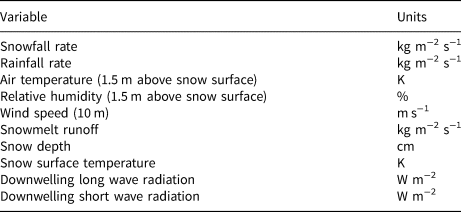
With the criteria set out above in mind, the geophysical array was designed to be an ‘inverse borehole’ with electrodes arranged on poles that would be gradually buried by the snow through the winter. The array was composed of four poles, each with ten electrodes equally spaced up each pole, making 40 electrodes in total. The poles were constructed from 2 m long 32 mm diameter hollow poles made from white polyvinylidene fluoride plastic. The poles were arranged in a square with spacing of 75 cm (see Fig. 1). The spacing and size of the array was partly constrained by the size of the area available for installation, and partly due to the poles also having electrical resistivity electrodes attached to them (data not reported here).
Fig. 1. (a) Schematic of a pole showing SP electrode spacing and location of PT100 thermistors (only mounted on one pole). (b) Photograph of poles during installation in October 2018, with an early snowfall. Pole spacing is marked. Snow around the poles was disturbed during installation but was expected to thaw before lasting snow fell later in the autumn. Electrical resistivity electrodes are also visible. These data are not reported here. (c) Close up view of lead strip SP electrode.
The array was designed to replicate the potential amplitude manual survey method set out by Corry and others (Reference Corry, Demoully and Gerety1983) and adapted to glacial snowpacks (Thompson and others, Reference Thompson, Kulessa, Essery and Lüthi2016). This method employs a fixed reference electrode buried near to, but outside of, the main survey area, and then a roving electrode which is used to measure the SP over a regular grid. Since ours was a monitoring study, instead of having a roving electrode, multiplexer chips were used to switch measurements between a regular array of electrodes.
By having electrodes spread on four poles in a square it was hoped that differences in readings between poles could be related to lateral differences in meltwater percolation in the snowpack. Similarly, the differences between readings from electrodes at different heights were intended to be related to the motion of meltwater on its journey from surface melt or rainwater input to basal runoff.
It is recognised that point measurements such as the SP measurements and the meteorological and hydrological data they were compared to are likely to exhibit differences due to heterogeneities across the site. By siting the array in an open and level part of the site, the data will be representative of the wider site.
Reference electrodes
The reference electrodes were non-polarising lead/lead-chloride SP electrodes of the Petiau type (Petiau, Reference Petiau2000) buried next to the main array ~10 cm deep in the soil, which was considered to be sufficiently deep, as thermal effects from diurnal heating were not a concern when the ground was covered in snow. Petiau electrodes were used for the reference electrodes because they produce stable readings over longer periods. They have a porous end which needs to remain damp to maintain good electrical contact, and because they were buried in the soil this condition was met over the winter period.
Pole electrodes
Petiau-type electrodes are too big to mount on poles. Manufacturing smaller bespoke Petiau-style electrodes was considered (as in Kulessa and others, Reference Kulessa, Chandler, Revil and Essery2012), but they also need to be kept damp to maintain electrical contact. This would not be possible for extended periods of time above the snow as the snowpack builds up before burial. Therefore, the electrodes for the poles were manufactured from lead sheeting and mounted on the poles. Kulessa (Reference Kulessa2003) used solid lead electrodes for monitoring experiments over a whole year. This corroborated their water bath testing and general expectations that lead is inert and non-polarisable. The lead strip electrodes employed here gave stable SP readings in water baths for several days. A lead electrode is shown in Figure 1c. They were constructed as strips of lead wrapped around the pole to provide a large surface area for contact with the snow, while remaining flush with the pole to reduce the possibility of snow compaction ripping them off.
Wiring arrangement
The electrodes were wired up to form 43 pairs of electrodes between which differential voltage measurements were made. These consisted of three reference pairs between the six reference electrodes, and then 40 dipoles between a reference electrode and a pole electrode. Three pairs of reference electrodes were required because three multiplexer chips were used. The measurements were made using a Campbell Scientific CR1000 datalogger, with multiplexer chips used to switch between the pole electrodes.
Temperature measurements
In addition to the SP measurements, two PT100 thermistors were mounted on one of the poles, one at ~30 cm height and one at 60 cm height. The PT100 thermistors were found to be useful to help verify whether the lower electrodes were buried or not. This was not possible by viewing the webcam images alone.
Data collection and processing
SP voltages were measured every 5 s between all 43 pairs of electrodes. The PT100 temperatures were measured once per minute. SP was measured at each electrode giving 40 SP values. Data measured at 5 s intervals showed diurnal and shorter-term variability overprinted on longer-term SP changes. To remove this shorter-term high-frequency variability and longer-term changes, the data were detrended, and then averaged at a 30 min interval. This preserved the diurnal fluctuations in the signal that we could relate to meteorological and hydrological data available to us.
Results from winter 2018–19
The system was installed at the end of October 2018. There were some short-lived shallow snowfalls in October and November, then lasting snow fell in December. It was not of sufficient depth to cover the array until further snowfall during January and early February. Snow depth reached a maximum of ~165 cm during early February, which completely buried the poles. It then compacted and thawed through the rest of February with the exception of two small snowfalls. Some snowfall in the first half of March was followed by a prolonged period of melt. There was another snowfall in early April of ~40 cm which reburied the lower electrodes meaning SP measurements were possible for a longer proportion of the melt season (see Fig. 2). Here, we introduce results from two periods of particularly insightful snowpack conditions and compares the SP measurements to the concurrent hydrological and meteorological conditions.
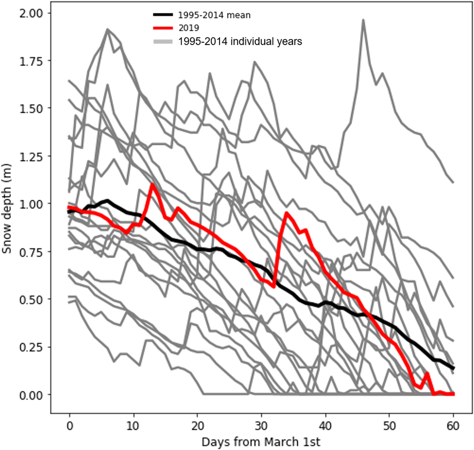
Fig. 2. March and April 2019 snow depth at Col de Porte plotted alongside 1995–2014 and long-term mean.
Uncertainty and error quantification
Reference measurements, dry snow and free air measurements
The reference measurements were generally stable, although some high frequency variations were present in the raw data. The reference readings had no notable diurnal (or other period) cycles apparently. Table 2 shows the mean and std dev. of the reference electrode measurements. Reference 1 showed more variation than 2 and 3 with a std dev. of 29.9 mV versus 10.8 mV and 4.8 mV respectively. Once the reference readings had been smoothed in the same way as the pole readings, the variation was negligible compared to the magnitude of the signals associated with meteorological and hydrological factors seen in the pole readings. Figure 8 shows the SP signals associated with electrodes melting out and being exposed above the snow surface. Once the electrodes are exposed a diurnal cycle is not visible.
Table 2. Mean reference voltage and std dev. for 21 March–14 April 2019

Figure 3 shows the difference between SP signals measured within the snowpack and above the snow exposed in air. It is clear that the measurements in air are noisier, and they do not exhibit cycles such as the clear diurnal cycle visible in the buried SP measurements. The standard error of the mean of the measurements in the snow is smaller than the measurements in the air.

Fig. 3. Example period from late March to early April 2019 showing difference between SP measurements in the snowpack and exposed in air above the snow. Standard error of the mean plotted in thin line style. Note the difference in error magnitude for electrodes buried versus electrodes above the snow. Above snow mean error for this period is 146.2 mV compared with 20.6 mV when buried in snow.
Figure 4 shows measurements from electrodes buried in cold dry snow. There is still an SP signal being generated, but it does not exhibit a diurnal cycle as the snowpack was not experiencing any melting. The magnitude of the SP signal is ~30–50 mV which is lower than the magnitudes of variations observed when a clear meltwater signal was present in late March and mid-April.

Fig. 4. Example period from late January 2019 showing the signal from electrodes buried in dry cold snow, with standard error of the mean plotted with dotted line. Mean error over this period in dry snow was 13.2 mV.
Lateral and vertical variation in readings
As described above, it was hoped that lateral and vertical differences would be discernible in the measurements. Unfortunately, it was impossible to discern any coherent lateral differences between the four poles. Similarly, coherent vertical differences in timing were not visible in the data from electrodes at different heights within the snow, although it was possible to differentiate between those electrodes that were buried and those that were not (Fig. 3). Because of this, the analysis that follows concentrates on mean measurements from the four electrodes at each height, and does not consider vertical or lateral changes in the signal.
SP signals during diurnal melting in spring
Meteorological and snow cover conditions in March 2019
March 2019 gave mixed conditions with some periods of snowfall, some rainfall, but temperatures often above freezing (see Fig. 5). Snow depth was around average for the time of year compared to previous years (Morin and others, Reference Morin2012; Lejeune and others, Reference Lejeune2019) (see Fig. 2). During late March, there was a prolonged period of snowmelt following a clear diurnal cycle. This was caused by a period of anticyclonic atmospheric conditions giving warm sunny days with ablation driven by solar radiation, and cool or cold nights with conditions ideal for radiative cooling and overnight refreezing. Air temperatures in the middle of the day reached as high as 15°C, but snow-surface temperatures overnight fell to below minus 10°C on several nights (see Fig. 6b). This period of marked diurnal melt/freeze cycling persisted into early April. During this period, snow depth was initially ~90 cm, falling to ~60 cm by the end of March. In Figure 5, this period of snowmelt is clearly seen from around 21st March in the observed snow depth, accompanied by predominately positive air temperatures. Thawing takes place every day from this date onwards. Figure 6b shows the snow-surface temperature reaching 0°C each day, indicating thawing is taking place. Within the snowpack, the temperature remained close to 0°C, which supports the assumption made earlier that thermoelectric potentials will be negligible within the snowpack. As the snow depth reduced, the PT100 sensor mounted 60 cm above the ground became exposed and recorded positive temperatures in the daytime when exposed to solar radiation. Although thawing is occurring at the snow surface every day during this period, there is a slight lag before runoff starts being recorded in the lysimeters (Fig. 6d). From around the 24th March onwards, a daily peak of runoff is observed, increasing to a peak flow of ~2 kg m−2 h−1 by the end of March. This shows that the snowpack is able to support liquid water flow through its full depth from around 24th March onwards.
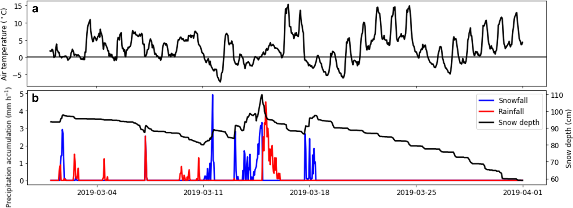
Fig. 5. (a) Observed air temperature at Col de Porte for March 2019. (b) Observed precipitation and snow depth at Col de Porte.
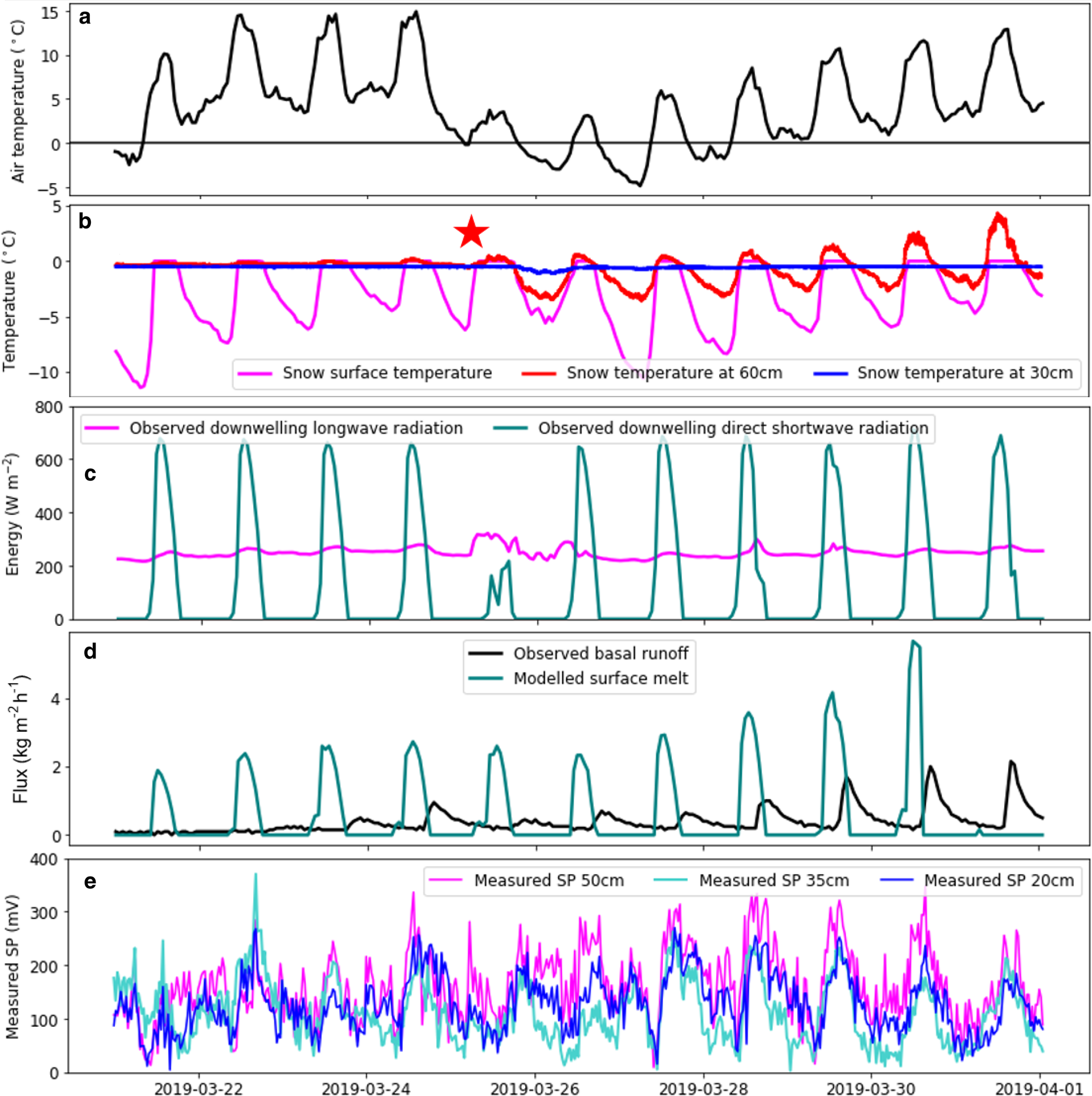
Fig. 6. Meteorological, hydrological and SP measurements for late March 2019. (a) Observed air temperature. (b) Observed snow surface temperature, and temperatures measured using PT100 thermistors at 30 and 60 cm above ground level for late March 2019. The red star indicates the approximate time from which the 60 cm thermistor was exposed (see cavities in Fig. 9). (c) Observed downward longwave and shortwave radiation. (d) Observed basal runoff from Meteo France lysimeter, and modelled FSM surface melt. (e) Mean SP from the four electrodes at each height buried in the snow. The mean standard error of the mean over this period was 39.9 mV at 50 cm, 21.4 mV at 35 cm and 23.5 mV at 20 cm.
Dye-tracing experiments carried out on the 19th and 20th March (Fig. 7) show that most of the snowpack was able to support meltwater flow. In these qualitative experiments to investigate the meltwater percolation, several layers were visible, and vertical and horizontal flow and preferential flow fingers were observed. It was found that dye reached the lowest layers of the snowpack in 2–3 h, but instead of continuing to percolate to the base of the snowpack, it then flowed horizontally down a slight gradient along a layer interface, marked in Figure 7. This layer interface was at ~15 cm above the ground so was below the lowest SP electrode on the pole but above the reference electrodes. Snow pit observations established that there were no ice layers or lenses at this depth in the snowpack, and that the interface that the dye flowed along marked a relatively small change in density, but with similar size snow grains. The stratigraphic contrast was also observed in snow pit observations on 28th March, albeit with a smaller density contrast. This was ~5 d after the lysimeters started to record runoff, showing that despite the layer interface persisting, the snowpack could support water flow right to the base.

Fig. 7. Dye-tracing experiment carried out on 20th March 2019. The density contrast, along which horizontal flow occurred, is marked.
Measured SP signals during late March 2019
As discussed above, the snowpack was able to support liquid water flow during late March. Therefore, we expected to be able to measure SP signals generated by this fluid flow in the snowpack. Preferential melting had occurred around the poles so the snow depth covering the pole was lower than the measured snow depth elsewhere. With a snow depth of ~90 cm at the beginning of the period, the top five SP electrodes on each pole were exposed, and by the end of the period with a depth of 60 cm, only the lowest three electrodes were reliably buried by the snow. Therefore, the data from the top seven electrodes on each pole were neglected. From Figure 1, it can be seen that the three lowest electrodes on each pole are at heights of 20, 35 and 50 cm above the ground.
In Figure 6e, a diurnal pattern is visible in the signals from the buried SP electrodes at the three lowest heights on the poles. Some days exhibit multiple peaks, and especially towards the end of the period, a clear daily signal is visible. The peak of the cycles are generally during the afternoon, with the minima overnight. This supports the assumption that the SP peaks are caused by diurnal melt flow. The peaks of each diurnal cycle increase in magnitude from around 24th March, which is when the lysimeter started recording runoff. However, the fact that there is still a diurnal peak before then supports the assumption that early in the period the SP signals are being generated by internal melt flow which is not reaching the base of the snowpack.
SP signals during a rain-on-snow event
Meteorological and snow cover conditions in mid-April 2019
After the period of prolonged melt in late March, heavy snowfall occurred early in April which increased the snow depth to ~110 cm. Further periods of thaw and some further snowfall occurred through to mid-April. Late on the 9th April, there was a small rain-on-snow event, then on the afternoon of the 10th April there was another, larger rain-on-snow event. There was no snowfall during this period. Figure 8b shows the air temperature remaining above freezing during and after these rainfall events. Snow surface temperature remained at 0°C until the night of the 12th April, so thawing can be assumed to have been taking place until then, with refreezing taking place that night followed by melting again the following day. Snow depth was initially ~70 cm on the 9th, falling to ~52 cm by the morning of the 13th. The temperature measured at 30 cm above ground remained ~0°C throughout, indicating that electrodes below that height would be buried. However, the PT100 at 60 cm recorded positive temperatures on each day, so it is assumed that electrodes around this height were not completely buried by the snow. Figure 9 shows a snapshot from the Meteo France webcam on 12th April. Cavities around the poles are visible, which explains why the electrodes and upper PT100 were not buried despite the observed snow depth nearby being sufficient earlier in the period.

Fig. 8. Meteorological, hydrological and SP measurements for April 2019. (a) Observed air temperature. (b) Observed snow surface temperature, and PT100 temperature on poles at 30 and 60 cm. (c) Observed snow depth. (d) Observed incoming long- and shortwave radiation. (e) Observed rainfall, modelled surface melt and observed basal runoff. (f) Mean observed SP signal from all electrodes at 35 and 50 cm. Mean standard error of the mean for this period was 55.5 mV at 35 cm and 32.6 mV at 50 cm.
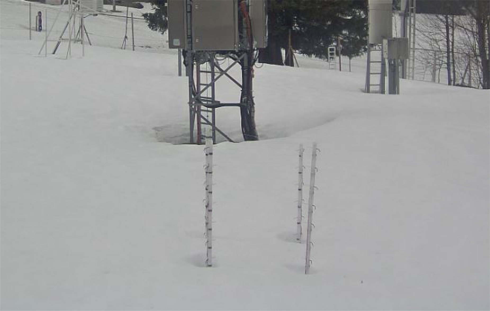
Fig. 9. Meteo France webcam image from midday on 12th April showing preferential melting has created cavities around the poles, exposing more electrodes than might be expected from the observed snow depth.
Figure 8e shows the observed rainfall, along with measured basal runoff and modelled surface melt. A clear peak in runoff is visible after each rainfall event. These peaks do not occur during the mid-afternoon as would be the case from diurnal melting. Before the first peak (runoff 1) there is a peak in modelled surface melt which will have supplied some liquid in addition to the rainfall at rain 1. The second peak (runoff 2) follows rain peak 2, and in this case there is no surface melt input. For runoff peaks 3 and 4, the runoff reverts to a diurnal cycle driven by solar radiation, which can be seen from the shortwave radiation and air and snow temperature peaks, although this is not reproduced by the model. Both the lower PT100 measurements and the Meteo France snow profiles carried out nearby show an isothermal snowpack at 0°C which could therefore support meltwater percolation to its base.
Measured SP signals during mid-April 2019
As discussed above, by mid-April the snow depth was not sufficient to cover many electrodes, with the preferential melting that occurred around the poles reducing the buried electrodes to those at 20 and 35 cm. Unfortunately, the measurements from the lowest level (at 20 cm) had shown evidence of longer-term changes in the SP signal by this stage of the season. We were unable to relate these changes to the observational data available. The electrodes at 35 cm appeared to give plausible readings, so the discussion of the rain-on-snow event and its SP signatures refer to measurements made at this level. The data from the electrode at 50 cm have been left in Figure 8 to show the response as it melts out and becomes uncovered.
In Figure 8f, a small peak (SP 1) in SP is visible on the evening of the 9th which occurred during the first period of rainfall. The associated peak in runoff (runoff 1) is slightly delayed from the peak in rainfall (rain 1), reflecting the time required for the water to percolate to the base of the snowpack. On the 10th, two SP peaks are visible. The first (SP 2) is smaller and occurs around noon. This is due to surface melting taking place. The air temperature was above freezing along with a peak in incoming shortwave radiation, and the snow surface was at 0°C. The second much larger peak (SP 3) occurs at the same time as the second rainfall event (rain 2), which was heavier than the first with hourly accumulation of over 6 kg m−2 compared to ~2 kg m−2 for rainfall 1. The peak in runoff (runoff 2) begins to occur before the rainfall, so it was probably registering runoff from surface melt first, and then percolation of rainwater. A further small peak (SP 4) is registered in the SP signal during the evening of the 11th, and it is not clear why this did not occur earlier when more melting will have been taking place. The runoff follows a similar pattern however, with a small peak (runoff 3) on the evening of the 11th too. Then, on the 12th, surface melting drives a broad peak in the SP signal (SP 5), which occurs just before a large peak (runoff 4) is recorded in the runoff. From the 13th onwards, it is not clear if the electrodes were sufficiently buried in the snow to make sensible measurements.
Discussion
In this section, the success of the SP measurement array in seasonal snow is evaluated against the scientific aims defined above. The system's utility in detecting snowmelt percolation events is discussed. Finally, an outlook is given for future research in seasonal snow building upon this feasibility study.
Monitoring SP signals of melting seasonal snow
With respect to the aims set out above, SP signals were successfully measured for a winter season at an Alpine site. Some gaps in the data were present due to power outages, and a significant amount of the data was not used because the snow cover was not deep enough to cover all the electrodes. However, for two interesting periods of snow conditions enough data were available to investigate the associated SP signals.
The system was designed to withstand the demands of an alpine winter season, and it did generally prove to be durable enough. However, by the end of the season it was clear that the poles had moved due to a combination of ground heave, and snow settling and movement. Due to the gentle slope in the topography, snowpack crept along this gradient over the course of the season. This bent the poles and moved one of them several centimetres further into the ground than when initially installed. The electrodes themselves remained well-attached to the poles and provided stable readings, although the drift noted in the lowest layer of sensors by the April rain-on-snow event was an exception. It is possible of course that many more electrodes would have recorded drift or spurious readings if they were buried in the snow for longer, but when they were in the open air the readings were noisy and subject to temperature fluctuations (as high as tens of degrees Celsius on sunny days followed by clear nights) so any drift was difficult to distinguish from other effects.
During the period of diurnal melting driven by solar radiation in late March, a clear diurnal cycle was visible in the SP signals, which ties in with expected generation of surface melt. SP signals were registered within the snowpack before runoff was detected in the lysimeters, showing the utility of the SP method as an internal meltwater flow sensor. The signals from the three different heights of measurement did not show any evidence of the highest sensors registering a signal first, followed by the lower ones as meltwater percolated vertically through the snow. The dye-tracing experiments showed the high speed of water percolation in this ripe snowpack which could explain the coincidence of peaks at all three levels. However, a more likely explanation is due to preferential flow along and near the poles delivering meltwater past the electrodes at roughly the same time. Additionally, the depressions that formed around the poles may have helped meltwater to preferentially flow towards and down the poles. In this context, although the method was as non-invasive and non-destructive as possible, it is likely that the measurement equipment has influenced the measurements to some degree.
In the rain-on-snow event that occurred in mid-April, clear peaks in the SP signal were attributable to both rainfall percolating through the snow, and subsequent surface melting due to positive air temperatures. However, by this stage in the season, preferential melting around the poles had exposed all but two levels of electrodes, and one of these levels had begun to give spurious readings. It was still possible to see clear peaks in the one remaining level of usable data though. The SP peaks occurred earlier than the lysimeters registered peak runoff, again showing the utility of the SP method as a sensor of internal flows. With only one level of electrode data available, it was not possible to compare peaks in SP at different levels, but it is expected that the same preferential flow will have occurred close to the poles.
Key limitations and advantages of the system
After the deployment of the system for a winter season, it is possible to assess the limitations and sources of uncertainty in the measurements made, and also to note the advantages such a system holds over traditional measurement technology.
After this preliminary experiment, it is clear that the SP system required a deep snowpack in order to bury enough electrodes to get usable readings. For a significant part of the winter season, right through to January, the snowpack was not deep enough to bury enough electrodes. Later in the season, the problem of preferential melting around the poles became more of an issue, with over 50 cm of observed snow not enough to bury more than the lowest electrodes. This preferential melting, causing depressions around the poles, may have contributed to preferential flow occurring along the poles. However, despite these limitations, some useful data were measured which could be related clearly to meteorological and hydrological factors.
The long-term drift in some of the readings which affected the April rain-on-snow data was investigated and there was not a clear cause. It was not related to some electrodes being connected to one multiplexer, as the four electrodes at that height were connected to three different multiplexers and three different reference electrodes and all exhibited similar drift. Poor electrical contact could have developed through air gaps melting, or it is possible that the electrodes at that level had been damaged through snow creep and compaction. This could have affected the connection to the electrodes or the cables attaching them, but it was not possible to verify this with a site visit.
The data measured on the poles showed fluctuations at high frequencies. It is difficult to attribute these fluctuations to issues with the electrodes which may have developed over the length of the winter season without having other electrodes or locations to compare to. It is worth noting that the reference dipoles composed of Petiau electrodes were very stable throughout, with little to no drift. It is not clear whether air gaps developed around the electrodes, and is therefore difficult to assess the quality of the electrical contact between snow and electrodes. This could have contributed to the high-frequency fluctuations which were observed. The array was sited by necessity in a location with a number of sources of electrical noise, from both buildings and equipment at the Centre d'Etude de la Neige, and the adjacent ski lift infrastructure. It is therefore likely that these high-frequency fluctuations were caused by a combination of poor electrical contact, electrical noise from the surroundings and poorly understood electrode drift effects.
Spatial variability was observed between the SP array and the Meteo France observations. This was most apparent in the snow depth, where differences between the Meteo France measured snow depth and that observed at the poles were greater than 20 cm by 12th April. Although clearly the internal structure of the snowpack will have varied across the site, we assumed that surface melt and precipitation inputs were constant across the site in our analysis, and this will have contributed to uncertainty.
Despite these limitations, the system showed advantages over other measurement systems. It was able to detect meltwater percolation within the snowpack before it reached the lysimeters. This is a key advantage, as timing of wetting front propagation through snow is very difficult to measure non-invasively. However, the likelihood of preferential flow along the poles precludes any significant conclusions being drawn regarding meltwater timings, along with the fact that vertical differences in readings were not coherent. However, the SP system was able to carry out bulk measurements of meltwater timings with some success, especially in the late March melting period. An advantage of this system over more complex ones is its simplicity and low cost. The electrodes, poles and cabling were easy to manufacture, and data loggers are relatively inexpensive to purchase. Due to this low cost, it would be possible to deploy SP arrays at a number of sites with relative ease.
Co-location of the SP system at the Col de Porte observatory provided high-quality meteorological and hydrological observations, which were essential to understand processes affecting the SP signals. Without these, a full suite of observational equipment would have needed to be installed in order to fully interpret the SP results.
Possible future research and developments
It is possible to note some improvements which could be made to the system to address some of the limitations outlined above. Clearly, the number of electrodes which were actually buried in the snowpack was too low, so an obvious improvement would be to position more electrodes lower on the poles, and put them closer together. For a site like Col de Porte, even if the maximum snow depth is enough to bury the poles, for most of the winter the poles will be exposed to some degree. To avoid the poles influencing the meltwater flow as much as possible, instead of mounting electrodes on poles one above another, poles of varying heights could be installed, with one electrode at the top of each pole. This would be similar to snow temperature sensors used in Switzerland as part of the IMIS network (Lehning and others, Reference Lehning1999). Although similar preferential flow and melt problems would undoubtedly be experienced to a degree, this style of installation could mean that the snow above the electrodes remained undisturbed.
To reduce noise, siting the array in a more electrically quiet location would go some way to helping this, but in reality this may not be practical. Sites with the requisite infrastructure and power availability are likely to be electrically noisy environments. To mitigate this as much as possible, future installations should include steps to quantify the noise present, so that some of it can be subtracted from the signal. Improving electrode siting may also help reduce noise, as noise is likely to be less of an issue if electrical contact is better.
Although the remotely programmable logger set up was useful, the hard-wired multiplexer layout was a constraint. In future, a more flexible arrangement would allow for different combinations of dipoles to be measured, and easier identification of problem electrode pairs.
The difference in noise levels between the Petiau electrodes in the soil, and the lead strip electrodes on the poles was significant. Manufacturing smaller bespoke Petiau-style lead/lead chloride electrodes for mounting as the pole electrodes was considered, as in the laboratory experiments in Kulessa and others (Reference Kulessa, Chandler, Revil and Essery2012), but it was decided that this type of electrode would not be reliable if exposed to the open air and repeated freezing and thawing cycles. It is possible that a better design using lead, or medical grade electroencephalogram materials would be possible, however the issue of electrical contact will always be an issue with electrodes that are left in situ for long periods. Siting one electrode at the top of each pole could address some of these problems as discussed above.
SP measurements could be combined with temperature measurements at each electrode using thermistors. This would enable verification of when liquid water flow is possible, improving interpretation of the SP signals. Future experiments could use lysimeters within the snowpack to better quantify how much flow is occurring and how this relates to the SP measurements, although this would be a destructive measurement and would not be suited to a monitoring campaign.
A key future direction of SP measurements in snow will be to compare modelled SP signals to those measured. Studies by Kulessa and others (Reference Kulessa, Chandler, Revil and Essery2012), Thompson and others (Reference Thompson, Kulessa, Essery and Lüthi2016) and Clayton (Reference Clayton2021) have proven the utility of using electrical models to use SP signals to infer snow hydrological properties in the laboratory and in the field. This feasibility study has shown that longer-term in situ monitoring of SP can work. State of the art energy-balance snow physics models can predict internal water fluxes in snow, but are very difficult to verify with measurements. Ongoing research is looking to couple electrical models of snow to energy-balance snow physics models. By comparing predicted SP signals to those measured through the snowpack during melting or rain-on-snow events, it may be possible to improve the way that models simulate internal water flux, and thus improve the overall performance of snowmelt runoff predictions, with obvious advantages for those reliant on snowmelt runoff forecasts for assessing flood and avalanche risk.
Conclusions
In this study, a preliminary installation of an SP monitoring array for seasonal snow was introduced. Some data from a field season at Col de Porte in the French Alps were discussed. These data showed the SP method's utility as a sensor for internal water flow in snow, using simple, low-cost equipment. The system was able to detect meltwater flow in response to diurnal melt cycles, and successfully detected rainwater percolation during rain-on-snow events. Although the data were noisy and limited in the number of electrodes able to provide useful data due to snow depth, the system has shown the potential of SP measurements in future snow science research. The system's ability to detect water flow within the snowpack before it was registered in conventional lysimeters shows the most promise for future development. By coupling an SP system to a high-resolution snow physics model, it may be possible to improve our ability to model the timing of meltwater fluxes through seasonal snowpacks. It is important to consider that, like all geophysical methods, SP measurements should not be considered a stand-alone tool. This method has been shown to have potential to improve our understanding of liquid water dynamics in snow when used in conjunction with a wide range of other measurement techniques. Combining SP measurements with models could show the most promise for improving our ability to predict snowmelt runoff timing, and thus give wide and significant benefits to those who rely on seasonal snow for their water supply, or are at risk of hazards associated with it.
Acknowledgements
This research was carried out as part of a NERC E3 Doctoral Training Partnership studentship under grant NE/L002558/1, in partnership with British Geological Survey who provided additional CASE funding. The authors thank the staff at the Centre d'Etude de la Neige for their invaluable contribution to the success of this study, especially Mathieu Fructus and Marie Dumont. Colin Kay and Alan Hobbs at the NERC Geophysical Equipment Facility gave excellent advice and manufacturing expertise.


 Open access