


I. Introduction
Recent observations using the electronically scanned microwave radiometer (ESMR) on board the Nimbus-5 satellite over the continental ice sheets of Greenland and Antarctica (Reference Gloersen, Gloersen, Wilheit, Chang, Nordberg and CampbellGloersen and others, 1974) have been puzzling in that there is a complete lack of correlation between microwave brightness temperature and physical surface temperature in Greenland, whereas in Antarctica there is a loose correlation over wide areas. This has provided an additional incentive for developing an applicable analytical model for explaining the microwave emission from snow and glacier ice. In addition, other experimental observations made on board aircraft sensor platforms over smaller glaciers, snow fields, and sea ice have been difficult to interpret in terms of existing models.
A useful insight into the microwave emission from snow fields has been provided by a macroscopic volume scattering model (Reference EnglandEngland, 1974), which was also developed for other solid dielectrics such as moist soil. England’s treatment involves specifically a parameter called the volume-scattering albedo, ω0, which is the ratio of the volume-scattering coefficient to the total-extinction coefficient. The extinction coefficient includes both the resistive losses and the scattering. The analysis involves specifying a value for ω0 and then computing the brightness temperature or emissivity based on this single parameter. The model may be used to calculate the emissivity or the brightness temperature of finite slabs of snow and ice with varying composition.
In this paper, a snow-particle scattering model using a microscopic approach is developed in which it is assumed that the snow field or snow cover consists of randomly spaced scattering spheres which do not scatter coherently. These assumptions then permit the utilization of the Mie scattering theory (Reference StrattonStratton, 1941, p. 563–73; Reference DeirmendjianDeirmendjian, 1969, p. 11–19, 119–24; Van de Reference HulstHulst, 1957, p. 119–30) in computing ω0 and its several components. The treatment is similar in many respects to that used in calculating microwave and optical properties of clouds (Reference Gaut and ReifensteinGaut and Reifenstein, 1971; Reference Curran, Curran, Kyle and MeyerCurran and others, 1975). One important similarity is that the particle size is comparable to the wavelength of the microwave radiation within the particle in both cases, since the particle sizes encountered in snow fields are sufficiently larger than cloud droplets to compensate for the lower index of refraction of the ice particles. An important difference in detail of this treatment is that the imaginary part of the dielectric constant of ice is orders of magnitude smaller than for water droplets, grossly reducing the absorption cross-section of the particle.
The snow-particle scattering model provides many more reflecting surfaces than any reasonable multi-layer model (resulting from seasonal snow accumulations or melting) or variable dielectric model would provide. Consequently, the Mie scattering effects should provide the major contribution to the volume extinction coefficients at the microwave wave-lengths and sub-surface snow-particle sizes encountered. The results show that the penetration depths vary from 10 to 100 wavelengths depending on the snow and ice conditions encountered. Thus, the effects of snow cover dominate in most observations of snow-covered glaciers at the wavelength of 1.55 cm used in the Nimbus-5 ESMR.
2. Analytical Approach
The far-field solution for scattering of electromagnetic waves by spherical particles was obtained by Reference MieMie (1908). Since the snow and ice fields of interest generally consist of non- spherical particles that are not well separated, two assumptions are required for application of the Mie theory. It is first assumed that the scattering particles are spherical. Secondly, it is assumed that the particles scatter incoherently and independently of the path length between scatterers. These assumptions are not expected to influence the qualitative nature of the results. The Mie theory is then used to calculate the extinction and scattering cross-sections of the individual particles as a function of particle radius and the complex index of refraction for given wavelengths λ. Subsequently, these quantities are used to solve the radiative transfer equation within the snow medium and calculate the radiative emission from the model snow-field surface.
The extinction cross-section σe, scattering cross-section σa and absorption cross-section σa for particles of radius r and the complex index of refraction r can be written as:


and
where a m and b m are the complex Mie scattering coefficients which contain Bessel and Neumann functions of ½ integer order. The coefficients are:


where λ is the free-space wavelength, r is the particle radius, n is the complex index of refraction, Im denotes a Bessel function of order m and Im denotes the corresponding Neumann function. The extinction cross-section for spherical ice particles with refractive index n = 1.78 +1 0.002 4, which corresponds to measured values in the centimeter wavelength range of pure water ice near its melting point (Gumming, 1952; Reference EvansEvans, 1965), is calculated for several wavelengths and particle sizes. The results of the calculations in terms of the extinction coefficient (see Equations (8) and (15)), are shown in Figure 1. By using this relatively high value of Im n, the importance of the scattering contribution to the extinction cross-section is emphasized, since it dominates even at this value of Im n. The computation illustrates the dependence of volume scattering on particle sizes in this wavelength range.
Although the added complexity of calculating for various profiles of temperature, snow density, and particle size with depth is well within the capability of the computational technique, a simplified model is constructed for the purpose of illustration (Fig. 2). A layer of uniformly sized spheres (the snow cover) of complex index n is situated on top of a perfectly absorbing medium (the glacier ice). The physical temperature in the snow cover is taken to be uniform at 250 K for simplicity. The actual temperature of the underlying glacier ice, taken to be 270 K, will be important only for very thin snow covers. Since the change in the dielectric constant from ice to air would give less than 10% reflectivity, and since the presence of the snow cover above both mitigates this abrupt dielectric change and introduces opacity between the ice and radiatively cold outer space, this model is reasonable except in the limit of vanishing snow thickness. Since the snow temperature is 250 K, the appropriate index of refraction is n = 1.78 + 10.000 5 (Reference CummingCumming, 1952). An additional simplification is that only the radiation emanating normal to the surface is calculated. In this case, the distinction between the two polarizations breaks down due to symmetry.

Fig. 1. Extinction coefficient as a function of microwave wavelength for several ice-particle radii.

Fig. 2. Sketch of model snow field overlying solid ice.
At microwave frequencies and at temperatures typical of the Earth and its atmosphere, the Rayleigh—Jeans approximation to Planck’s function is applicable, giving the thermal radiative intensity (radiance) from a black body as proportional to its temperature. For non-black bodies, or in general, the radiance is usually expressed as a brightness temperature T b, which is proportional to the physical temperature. Thus, the radiative transfer equation of Reference ChandrasekharChandrasekhar (1950, p. 8–14) with axial symmetry may be written as:

where z (the distance below the snow surface) is used instead of the optical depth
Also, γe, γs, and γa are the extinction, the scattering, and the absorption coefficients respectively, defined as
where N r is the number of particles of radius r per unit volume. The volume scattering albedo,
is independent of the density of scatterers. F(θ;, θs) is the scattering phase function which is defined as the fraction of incident energy scattered into unit solid angle about a direction which makes an angle Θ with the θ and θs:
where S 1(Θ) and S 2(Θ) are scattering amplitude functions


a m and b m are as defined in Equations (4) and (5); IIm and θm are functions of Legendre polynomials
Equation (7) is solved numerically after rewriting it as:

The right-hand side represents the angular distribution of radiation resulting from the scattering, and equals zero for a non-scattering medium. To solve the complete Equation (15), the snow cover is first divided into a number of smaller layers. Between 50 and 100 layers are chosen to maintain the optical thickness of each layer typically less than about 0.01, but as large as 0.05 for the snow covers having the highest optical thicknesses. The isotropic upwelling radiance at the bottom of the snow cover is given by the chosen lower boundary condition. In order to compute the angular radiance distribution term, the angular variable is divided into 20 equal intervals. The redistribution of the isotropic upwelling radiance by the lowest layer into the 20 angular intervals is determined by the scattering phase function, and the radiance scattered into each interval is summed. The calculation proceeds upward layer by layer. At each layer, the redistribution of the upwelling components from the previous layer is calculated. The downwelling components from each layer are stored for subsequent calculation. At the top layer, the boundary condition specifies that no downward radiation is received from outside the medium. The downwelling radiance is then similarly calculated downward layer by layer while storing the recalculated upwelling components. This procedure is reiterated, maintaining the boundary conditions, until the emitted radiance that is calculated on successive passes deviates by less than one kelvin; five passes were sufficient for all cases in this study. The method of solution is a variation of the Gauss-Seidel iteration (Reference HildebrandHildebrand, 1956, p. 439–43).
3. Computational Results
Using the formalism developed in the preceding section, the primary computational result is the brightness temperature of the snow surface normal to the surface. A set of brightness temperatures is calculated for wavelengths of 2.81, 1.55, and 0.81 cm, for snow-cover thicknesses from 10 cm to 20 m, and for ice-particle radii from 0.1 mm to 5 mm. The density of scattering particles N r depends on the particle radii as follows:
where P is the packing fraction (snow density/ice density).
A snow density typical of moderately packed snow (480 kg/m3) is chosen, giving N r = (2r)–3 for the computations. The calculated surface brightness temperatures are displayed in Figures 3, 4, and 5. In these figures, an asymptotic behavior is apparent when the thickness of the snow cover becomes large compared with the wavelength, implying that little radiation emanates from depths greater than the penetration depth defined by such asymptotic thicknesses. For a particle radius of 0.2 mm, which is typical of fresh snow, the asymptotic thickness is approximately 10 m for λ = 2.81 cm, 5 m for λ = 1.55 cm, and 2 m for λ = 0.8 cm. The asymptotic value of the brightness temperature as the snow thickness is increased depends only upon ω0, the scattering albedo. The asymptotic brightness temperatures calculated for 2.81, 1.55 and 0.81 cm wavelengths are plotted in Figure 6 as a function of ω0 Also shown is the emissivity (ϵ = T b(o, o)/T(o)) of the asymptotically thick snow cover.

Fig. 3. Surface brightness temperature as a function of ice-particle radius f or several values of the snow thickness and for a microwave wavelength of 2.81 cm.

Fig. 4. Surface brightness temperature as a function of ice-particle radius f or several values of the snow thickness and for a microwave wavelength of 1.55 cm.

Fig. 5. Surface brightness temperature as a function of ice-particle radius for several values of the snow thickness and for a microwave wavelength of 0.81 cm.

Fig. 6. Asymptotic brightness temperature and emissivity of the snow cover as functions of the volume-scattering albedo, wo = ys/ye. The values for all three wavelengths—2.81 cm (crosses), 1.55 cm (solid circles), and 0.81cm (open circles)-fall on the same cure.

Fig. 7. Volume-scattering albedo as a function of ice-particle radius for several values of the imaginary part of the index of refraction and for a wavelength of 2.81 cm.

Fig. 8. Volume-scattering albedo as a function of ice-particle radius for several values of the imaginary part of the index of refraction and for a wavelength of 1.55 cm..
The consequences of varying the index of refraction in the ice particles has also been examined. The impurity level in ice is known to affect the real part of the index only slightly. On the other hand, the imaginary part of the index varies by many orders of magnitude with the introduction of impurities in the temperature range 260–273 K (Reference Hoekstra and CappillinoHoekstra and Cappillino, 1971). While it is approximately 0.002 4 for pure ice near 0°C, it can be as high as 0.1 for first-year sea ice at the same temperature. Such variations are attributed to the lowering of the melting point of the ice and the existence of a two-phase system over a broader temperature range with the presence of metal salts. The variation of the imaginary part of the index of refraction leads to different values of ω0 for a given wavelength Λ and particle radius r. This is illustrated in Figures 7, 8 and 9 for the three wavelength values 2.81, 1.55 and 0.81 cm, respectively. These curves show that ω0 is a strong function of the loss tangent which, in turn, depends on the physical temperature of the snow. This suggests that in order to determine the ice-particle size by remote sensing, multi-spectral measurements are needed. Curves such as those shown in Figure 10, in which ω0 has been eliminated as an intermediate parameter from the curves of Figures 6–9, illustrate this requirement. Determination of the average particle radius from measurements of T b and an a Priori knowledge of the physical temperature would be straightforward using the curves of Figure 10 except for the complicating factors of particle-size variation with depth (to be discussed later), variation of penetration depth with microwave wavelength, and temperature gradients in the snow.

Fig. 9. Volume-scattering albedo as a function of ice-particle radius for several values of the imaginary part of the index of refraction and for a wavelength of 0.81 cm.
Values of the azimuthally integrated differential scattering cross-section, F(θ θs (see Equation (9)), have been calculated and are shown in dimensionless form in Figure 11. The data are parameterized in terms of the particle size parameter α = 2π/λ and are divided by 2πλ2 so that these are valid for all wavelengths. Note that for α = 0.02, the forward and backward scattering are essentially equal and the scattering to the side is about half as large. As the particle size increases, the near-forward scattering increases much more than the near-backward scattering. (Note the curve for α = 1. 12, Figure 11.) What is more important, however, is that the differential scattering cross-section increases rapidly as α increases, which accounts largely for the behavior of ω0 as a function of the particle radius (Figures 7–9). It can be seen from these curves that the scattering effects become significant for the lower values of the loss tangent when the particle radii are greater than a few hundredths of a microwave length.

Fig. 10. Emissivity of the snow cover as a function of ice-particle radius for three different values of the imaginary part of the index of refraction and for three different wavelengths
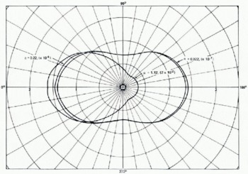
Fig. 11. Unit volume differential scattering cross-section for three different values of the particle-size parameter α. The quantities shown in parentheses are the scale factors to be applied to the r-axis.
4. Observations And Discussion
An example of the spectral variation in the microwave emission of a snow-covered temperate glacier is shown in Table I. By neglecting the temperature gradient in the snow, calculations from the simplified model can be used to determine the emissivity, and consequently the diameter of an average scattering particle. The emissivity is taken as the ratio of the brightness temperature to the physical temperature of the surface, obtained both by remote measurements with an airborne 10 pm radiometer and from surface reports (Reference Schmugge, Schmugge, Wilheit, Gloersen, Meier, Frank, Dirmhirn, anteford and SmithSchmugge and others, 1974). Assuming that the appropriate loss tangent for snow on a temperate glacier is 0.001 4 (Im n = 0.002 4), the curves of Figure 10 were used to obtain the particle radii also listed in Table I. Note that the average radius increases with the wavelength. Since the optical depth is greater for the longer wavelengths, the longer wavelength radiation is predominantly from greater depths where the snow grain sizes are larger, and the shorter wavelength radiation is from nearer the surface. These average radii are consistent with estimated grain sizes in the snow-pack which range in radius from 0.15 mm near the top to 0.5 mm at the bottom (private communication from M. F. Meier in 1974). Although the model calculations presented do not include variations in the grain size, temperature, and density with depth, the simplified model does provide emissivities for different grain sizes which are consistent with the observations and at least qualitatively correct for wavelengths up to 2.8 cm. For the longer wavelengths, part of the radiation emanates from the glacier itself, and curves such as those in Figures 3 to 5 apply.
Table I. Microwave brightness temperatures of the 8.4 msnow cover on south cascade glacier (station p–3, elevation 2 040 m, march 1971 data)

Since the microwave radiation emanates from a range of depths which depends on the microwave wavelength, the physical temperature gradient in the snow should have a wavelength-dependent effect on the brightness temperature. Therefore, if the physical temperature increases with depth, the brightness temperature should also increase with wavelength, as is generally observed above. However, since the observed 60 K. range in brightness temperature is considerably larger than any realistic range of physical temperature in the snow, the scattering effect must be dominant. Neglecting the temperature gradient is therefore justified in the foregoing analysis.
The computational results show that volume scattering from the individual grains is also a dominant factor in determining the emissivity of dry polar snow and firn, based on limited knowledge as to the particle sizes occurring in the snow cover. While this complicates the measurement of the near-surface temperature by microwave radiometry, it does provide a potential for measuring other parameters of glaciological interest, for example the extent of summer melting and snow accumulation rates.
As pure ice nears the melting point, the loss tangent increases rapidly. In fact, for the thin liquid film that forms on the crystals, the loss tangent reaches a value the order of 0.4. Under these conditions, the scattering albedo ω0 is nearly zero (Figs 7–9) and the emissivity is nearly unity (Fig. 6). This represents a plausible explanation of the sudden increase in brightness temperature of snow observed near its melting point (Reference Edgerton, Edgerton, Stogryn and PoeEdgerton and others, 1971; Reference Gloersen, Gloersen, Wilheit, Chang, Nordberg and CampbellGloersen and others, 1974). This effect should permit the mapping of the annual variations of the dry-snow zones versus percolation or soaked zones in Greenland, for example.
A more detailed rationale is required to show the relation between snow accumulation rates and microwave brightness temperatures. It is known (Reference GowGow, 1969, Reference Gow1971) that the crystal size in dry firn is a function of time t and temperature T:
where D 2 is the cross-sectional area at time t, D 0 2 is the initial cross-sectional area, k 0 is a constant, E is the activation energy of the growth process per unit volume, and R is the gas constant. Also, the age t of a crystal at a particular depth z is a function of the snow load σ and the mean accumulation rate A:

Fig. 12. Ice crystal radius as a function of snow depth for several values of the accumulation rate A and the average temperature T. The values of the temperature are not shown with error limits; the minus refers to the smaller value of A and the plus to the larger value. Note that the variation with accumulation rate of the ice crystal radius in each bracketed pair of curves runs counter to the trend that would be caused by temperature variation alone within that pair.
σ(z), which is the integral over the curve of density versus depth, also depends weakly on T and A. To illustrate that the dependence of σ (z) on A can be neglected, a comparison of Maudheim (lat. 71.0° S., long. 10.8° W.), where T = 256 K. and A = 37 g/cm2, with Wilkes (lat. 66.1° S., long. 11o.6°W., where T = 254 K and A = 13 g/cm2, indicates that the snow load at z = 25 m differs by less than 10% while A differs by a factor of three (Reference GowGow, 1968, Reference Gow1969). Therefore, for a given temperature, the profile of crystal size with depth depends on the accumulation rate, which is the parameter of interest:
One must, of course, take into account the difference between crystals and grains, which are typically composed of one or two crystals (Reference GowGow, 1969) and are a more likely measure of the size of scattering centers. However, grains and crystals have been observed to maintain a fairly constant mean size ratio of 1.4: 1 (Reference GowGow, 1969).
In general, the gradient of D 2(z) increases with increased T or decreased A, as can be seen from Equation (19). The dependence on A and T is clearly indicated in Figure 12, where crystal-size profiles obtained at four different field measurement sites are illustrated.
Now, for the range of grain sizes encountered, the corresponding portions of the emissivity curves of Figure 10 can be approximated by:
where D 2 = πr 2

Fig. 13. Contours of constant emissivity at a microwave wavelength of 1.55 cm on Greenland. The emissivity values were obtained by taking the ratio of the brightness temperatures obtained at wavelengths of 1.55 cm to those obtained at wavelengths of 10 μm from instruments on board the Nimbus-5 satellite. The data were obtained on a relatively cloud-free day (11 January 1973).
Since the curves of Figure 10 were calculated on the basis of uniform particle sizes, it is necessary to replace D 2 in Equation (20) by D 2, which is an average of Equation (19) over z, weighted by the radiative transfer properties. As A increases, both D 2 (Equation (19)) and D 2 will decrease and ε (Equation (20)) will increase. Therefore, emissivity and accumulation rates should be directly correlated over areas of constant temperature.
We have in fact observed a remarkable correlation between the brightness temperature contours of the Nimbus-5 ESMR (Reference Gloersen, Gloersen, Wilheit, Chang, Nordberg and CampbellGloersen and others, 1974) and the known accumulation rate patterns in Greenland (Reference MockMock, 1967) and Antarctica (Reference Bull and QuamBull, 1971), despite the fact that the spatial variations of the physical temperature are included. Since a 10% variation in emissivity is roughly equivalent to a 25 K variation in temperature, it is not too surprising that emissivity variations dominate.

Fig. 14. Contours of constant emissivity at a microwave wavelength of 1.55 cm on Antarctica. The emissivity values were obtained by taking the ratio of the brightness temperatures obtained at wavelengths of 1.55 cm to those obtained at wavelengths of 10 μm from instruments on board Nimbus-5 satellite. The data were obtained on a relatively cloud-free day (11 January 1973).
In order to make a more direct comparison between emissivity and accumulation-rate patterns, an approximate emissivity has been obtained, i.e. the ratio of brightness temperatures obtained at the wavelengths of 1.55 cm and 10 μm. Such values cannot be obtained consistently because of persistent cloud cover, but were obtained on 11 January 1973 for Greenland (Fig. 13) and Antarctica (Fig. 14). Again, the areas with the highest emissivities are approximately those with the highest accumulation rates. In making these comparisons, it is necessary to consider regions with similar physical temperatures due to its effect on the rate of grain growth. In particular, the emissivity in Greenland (Fig. 13) decreases from the central summit (ϵ = 0.85) to the northern region (ϵ = 0.70) which has lower accumulation. It is approximately constant (ϵ = 0.75) from north-west of the summit toward Camp Century (see Fig. 12) and increases from ϵ = 0.70 on the low accumulation area on the south-west to ϵ = 0.85 on the very high accumulation area on the south-east. In Antarctica (Fig. 14), the emissivity is low (ϵ = 0.70) over the low accumulation area in the central plateau of East Antarctica (vicinity of lat. 8o° S., long. 90° E.). It is high (ϵ = 0.85) in the high accumulation area at the base of the Antarctic Peninsula in contrast to a low value (ϵ = 0.70 to 0.75} in the West Antarctic region draining into the Ross Ice Shelf (vicinity of lat. 82° S., long. 140° W.). In both southern Greenland and the “Byrd” station region of West Antarctica (lat. 80° S., long. 120° W.), the T b contours are parallel to the ice divides, which also mark regions of differing accumulation rates.
In the case of the Lambert Glacier (lat. 72° S., long. 68° E.) in Antarctica, the emissivity is also high, about 0.85. It is known (private communication from W. F. Budd in 74) that this glacier has extensive areas of exposed blue ice due to vigorous wind action in the area; such areas would be expected on the basis of this model to have very low scattering albedo and hence high emissivity (sec Fig. 6). Thus, a high emissivity does not necessarily imply a high accumulation rate over a glacier. Therefore, some prior knowledge of the general characteristics of the snow field is required to interpret properly the observed brightness temperatures.
5. Conclusions
A microscopic model, which considers the individual snow grains as the scattering centers and employs Mie extinction and scattering coefficients, has been used to obtain a qualitative explanation of the low brightness temperatures observed over snow fields and snow-covered glaciers. More quantitative descriptions will be provided by this model when the vertical grain-size distribution, physical temperature, and variation in loss tangent are taken into account. The present work has given essentially the same results as Reference EnglandEngland (1974) obtained in terms of the variation of brightness temperature with the scattering albedo ω0 The results differ in detail, however, because England assumed isotropic scattering in his model; Mie scattering, assumed here, is anisotropic. An additional result of the present analysis is the determination of the variation of ω0 as a function of particle sizes, wavelength, and loss tangent. It has been shown that in the wavelength range from 0.8 to 2.8 cm, and for snow crystal sizes normally encountered, most of the microwave radiation emanates from a layer the order of 10 m or less in thickness. An additional important result of this analysis is the explanation of the signature of wet snow in terms of a wet surface on the snow grains, which causes a large increase in the loss tangent of the scatterers which, in turn, gives near-zero values for ω0, the scattering albedo. Finally, it is concluded that it may be possible to determine snow accumulation rates as well as near-surface temperatures by utilizing this model in conjunction with multi-spectral observations in the microwave region.


