


Introduction
Fresh water scarcity has been intensifying recently because of severe droughts brought by climate change, salinizing aquifers, food loss and waste, food system inefficiencies, etc. (Postel Reference Postel2000; World Economic Forum 2019). In the meantime, demand for water has been on the rise due to population growth, as well as expanding sectors of economies (e.g., agricultural production, food manufacturing, retailing, and foodservice) driven by intensive farming practices and economic growth (Harris Reference Harris2015). This has contributed to the heightened urban/agricultural conflict (i.e., residential water vs. economic resource uses such as agricultural production) and freshwater overextraction, which can adversely affect future water supplies and can endanger aquatic ecosystems (e.g., Postel Reference Postel2000).
Residential water use includes water for indoor household purposes (drinking, food preparation, bathing, etc.) and outdoor purposes (watering lawns and gardens). In the United States, about 88 percent of the residential water is provided by public suppliers, while the remaining 12 percent comes from self-supplied withdrawals by means of wells and rainwater collected in cisterns (Dieter et al. Reference Dieter, Linsey, Caldwell, Harris, Ivahnenko, Lovelace, Maupin and Barber2018a, Reference Dieter, Maupin, Caldwell, Harris, Ivahnenko, Lovelace, Barber and Linsey2018b). Specifically, in 2015, public suppliers provided upward of 23 billion gallons/day as domestic deliveries, which translated to a total per capita consumption of 82 gallons/day (Maupin et al. Reference Maupin, Kenny, Hutson, Lovelace, Barber and Linsey2014). In the meantime, the monthly water bill for an average US household of four with 100 gallons per person/day consumption totaled only $62.4, which may create an impression that households have little reason to respond to changing water prices (Circle of Blue 2019). However, it deserves mentioning that a considerable amount of residential water is used by a relatively small number of high-volume customers, who are impacted significantly by water price movements (Teodoro Reference Teodoro2018). Therefore, it is imperative to gain a clear understanding of the actual residential water demand structure and household price and expenditure sensitivity, which will improve the timeliness and effectiveness of public policies that strive to balance urban and agricultural water needs.
Residential water demand has been analyzed extensively in the previous literature. As summarized in a synoptic survey conducted by Worthington and Hoffman (Reference Worthington and Hoffman2008), the great majority of studies relied on the ordinary least squares (OLS) estimation method while utilizing household-level, community-level, or utility-level panel data. The consensus seems to be that users generally respond to price changes, whereas user sensitivity estimates have been mixed as it relates to the magnitude (i.e., both elastic and inelastic price elasticities). Similarly, income emerges as a significant determinant of residential water demand with its estimated magnitude indicating that residential water is a normal good and, moreover, it is a necessity. Finally, seasonality, household size, and the imposition of water use restrictions appear to be some of the important noneconomic factors affecting water demand. The predominant assumption in the previous literature has been that entire water consumption responds to price changes (Worthington and Hoffman Reference Worthington and Hoffman2008).Footnote 1 However, evidence suggests that some users are insensitive to changing prices before certain amounts of water are secured (i.e., precommitted demand), only beyond which price becomes an important consideration (i.e., supernumerary demand). In other words, precommitments take precedence over supernumerary demand and need to be fulfilled before one reaches the supernumerary or discretionary portion of demand, where price and income are the important demand drivers (Rowland, Mjelde, and Dharmasena Reference Rowland, Mjelde and Dharmasena2017). Most previous studies also suffer from the econometric issue of price endogeneity stemming from the omission of the supply side of the price determination mechanism, due perhaps to the lack of data on proper price instruments (see, e.g., Foster and Beattie Reference Foster and Beattie1979; Chicoine and Ramamurthy Reference Chicoine and Ramamurthy1986; Rietveld, Rouwendal, and Zwart Reference Rietveld, Rouwendal and Zwart2000). Finally, despite the findings by Abrahams, Hubbell, and Jordan (Reference Abrahams, Hubbell and Jordan2000), Zivin, Neidell, and Schlenker (Reference Zivin, Neidell and Schlenker2011), and Johnstone and Serret (Reference Johnstone and Serret2012) providing evidence for demand interrelationships between residential and bottled water, these two commodities have largely been studied separate from each other (e.g., Zheng and Kaiser Reference Zheng and Kaiser2008; Dharmasena and Capps Reference Dharmasena and Capps2012).
We examine the structure of demand for residential water in the United States while addressing some of these major issues that have plagued the previous literature within a single framework. Specifically, our study has four distinguishing characteristics. First, we model the demand for residential and bottled water jointly, in recognition of the possibility that both water types are substitutes/complements in consumption. More specifically, we employ a system's framework that not only accounts for demand interdependences, but also controls for unsuspected contemporaneous correlation between the unobserved demand determinants thereof. Second, we address simultaneity-induced water price endogeneity by adopting an empirical framework proposed by Dhar, Chavas, and Gould (Reference Dhar, Chavas and Gould2003). Specifically, we apply a full information maximum likelihood (FIML) procedure to the estimation of the system of demand and reduced-form equations that relate expenditure and water prices to the respective exogenous shifters (e.g., per capita income, industrial electricity prices, retail rents, respective wage rates), thus accounting for the supply side of price determination mechanism. Third, we exploit a Generalized Exact Affine Stone Index (GEASI) model that is a state-of-the-art demand system that allows for potential precommitted quantities in consumption, along with unobserved consumer and region heterogeneity, and unrestricted Engle curves for both water types (Lewbel and Pendakur Reference Lewbel and Pendakur2009; Pendakur Reference Lewbel and Pendakur2009; Hovhannisyan and Shanoyan Reference Hovhannisyan and Shanoyan2019). Fourth, our study encompasses a relatively larger geographical area vis-à-vis many similar studies in this line of literature. Specifically, our sample includes 26 major cities in the four broadly defined regions of the contiguous United States.
Our main findings indicate that residential and bottled water are substitutes in consumption. Further, significant precommitments are found in both residential (79 percent) and bottled water (23 percent) consumption, which diminishes the role of price-based water management and water policies aimed at balancing the water needs of different user groups. We also find that residential water users become significantly price-sensitive once the precommitted amounts are reached, while demand for bottled water is estimated to be price-insensitive. Finally, we demonstrate that ignoring demand interdependences between residential and bottled water, precommitted demand components, as well as expenditure and price endogeneity results in significant biases in estimated parameters governing water consumer behavior and price and expenditure elasticities.
The results from this study can potentially benefit water-regulating agencies in designing and setting water rates to improve consumer welfare by furnishing demand elasticities and identifying the level of water demand beyond which these elasticities take effect. The empirical findings can also benefit water supply operators in their pricing strategies and decision-making related to capital investment to maintain and upgrade the water supply infrastructure. Also, policymakers can glean valuable information from this study for the sake of evaluating the effects of various tax and water conservation policies.
The rest of the article proceeds as follows. The second section contains the description and the empirical specification of the model used in this study. The third and fourth sections present the data used followed by outlining the estimation procedure and the presentation and discussion of the empirical results. Concluding remarks and recommendations for future research are presented in the fifth section.
Methodology
In this section, we briefly present the GEASI demand system underlying our empirical analysis. It is based on the Exact Affine Stone Index (EASI) model of Lewbel and Pendakur (Reference Lewbel and Pendakur2009) and is extended by Hovhannisyan and Shanoyan (Reference Hovhannisyan and Shanoyan2019) to incorporate potential precommitments in consumption. Furthermore, we provide a brief description of water price and expenditure endogeneity. Finally, we discuss a FIML framework proposed by Dhar, Chavas, and Gould (Reference Dhar, Chavas and Gould2003) that is used to address the econometric issue of endogeneity.
A GEASI demand framework
Following Hovhannisyan and Shanoyan (Reference Hovhannisyan and Shanoyan2019), the GEASI budget share equations are specified as follows:

where w it is the budget share of product i in period t, c i is the precommitted demand for product i that is insensitive to prices and income movements,Footnote 2 X is the total water expenditures, p it is the price of product i in period t, ɛit denotes the unobserved water demand determinants, L is the highest order of polynomial in expenditures, $( {\rm ln}( X-{\tilde{c}}^{\prime}p) -{w}^{\prime}\,{\rm ln}\,p)$ is price and precommitment-adjusted total expenditure, c ′p represents precommitted expenditures, and αik, and βil are parameters to be estimated.
It is important to note that the GEASI model in (1) is subject to the classical theoretical restrictions of adding-up $\sum\nolimits_{i = 1}^N {{\rm \beta }_{i0} = 1; \;} \,\sum\nolimits_{i = 1}^N {{\rm \beta }_{il} = 0, \;\quad \forall \,l = 1, \;\ldots , \;L; } &eqnbreak;\sum\nolimits_{i = 1}^N {{\rm \alpha }_{ik} = 0} \quad ( {\forall \,k = 1, \;\ldots , \;N} )$ and symmetry ${\rm \alpha }_{ik} = {\rm \alpha }_{ki}( \forall i, \;k = 1, \;\ldots , \;N)$
 . In addition, regional fixed-effects reflecting region-specific unobserved demand determinants are incorporated into the GEASI system via demographic translating, i.e., $\tilde{c}_i = c_{i0} + \sum\nolimits_{r = 1}^{R-1} {c_{ir}} d_r$
 , where $\tilde{c}_i$
 is expressed as a linear function of regional dummy variables d r, R is the number of regions, and c i0 and c ir are parameters reflecting regional differences in water consumption (Pollak and Wales Reference Pollak and Wales1981; Tonsor and Marsh Reference Tonsor and Marsh2007). Finally, the GEASI demand system retains all the desirable properties of the Almost Ideal Demand model of Deaton and Muellbauer (Reference Deaton and Muellbauer1980) and similar demand models that have been used extensively in the consumer demand literature. It further improves upon the previous models in that it allows for unrestricted Engel curves and unobserved household preference heterogeneity (Lewbel and Pendakur Reference Lewbel and Pendakur2009; Zhen et al. Reference Zhen, Finkelstein, Nonnemaker, Karns and Todd2014).
To evaluate water consumer expenditure and price sensitivity, we use the respective elasticity formulas derived by Hovhannisyan and Shanoyan (Reference Hovhannisyan and Shanoyan2019). Specifically, the expenditure elasticity formula is derived from the GEASI budget share equations provided in (1) as follows:

where E is the (N × 1) expenditure elasticity vector with e i denoting its ith element, W represents the (N × 1) vector of observed commodity budget shares, ln p is the (N × 1) vector of logarithmically transformed prices, A denotes $\left({\sum\nolimits_{l = 0}^L {{\rm \beta }_{il}} {( {{\rm ln}( {X-{c}^{\prime}p} ) -&eqnbreak;{w}^{\prime}{\rm ln}p} ) }^l + \sum\nolimits_{k = 1}^N {{\rm \alpha }_{ik}{\rm ln}\,p_k} } \right)$ , B is a (N × 1) vector with its ith element represented by $\sum\nolimits_{l = 1}^L {{\rm \beta }_{il}ly^{l-1}}$
 , 1N is a (N × 1) vector of ones, and ° denotes the Hadamard–Schur product with t° p = [t 1p 1, …, t Np N].
Next, the GEASI-based Hicksian elasticity equations are derived as shown below:

where δij is the Kronecker delta that is 1 when i = j, and 0 otherwise, and A is defined above.
Finally, the Marshallian price elasticities $( e_{ij}^{\rm M} )$ are recovered from the Slutsky equation $( {{\rm i}{\rm .e} ., \;\,\,e_{ij}^{\rm M} = e_{ij}^{\rm H} ( {\rm \alpha }_{ij}/w_i) -w_je_i} )$
 using the Hicksian $( e_{ij}^{\rm H} )$
 and expenditure elasticity estimates (e i) as follows:

As illustrated by Rowland, Mjelde, and Dharmasena (Reference Rowland, Mjelde and Dharmasena2017), ignoring precommitted quantities (c i) when they are present can have a significant impact on the elasticity estimates. The intuition is that consumer lack of response to changes in economic variables over the precommitted portion of demand is ascribed to all consumption, which lessens the magnitude of elasticity estimates.
A FIML framework to addressing the endogeneity of water expenditures and prices
An important econometric issue that needs to be addressed in empirical demand studies is expenditure endogeneity. Specifically, water expenditure is endogenous because it appears on both sides of the GEASI specification in equation 1, implying joint determination of expenditure shares and total expenditures (i.e., w it = p itq it/X, where q it is the amount of water type i consumed in period t) (Dhar, Chavas, and Gould Reference Dhar, Chavas and Gould2003). Price endogeneity is yet another major problem requiring attention, since price affects water consumption and the latter can affect price because of the block rate nature of residential water pricing, thus resulting in simultaneity (see, e.g., Nieswiadomy and Molina Reference Nieswiadomy and Molina1989; Hewitt and Hanemann Reference Hewitt and Hanemann1995; Olmstead Reference Olmstead2009). Ignoring price endogeneity brought by simultaneity between price and consumption can substantially distort parameter estimates of consumer demand, resulting in erroneous policy advice (Nieswiadomy and Molina Reference Nieswiadomy and Molina1989; Dhar, Chavas, and Gould Reference Dhar, Chavas and Gould2003; Hovhannisyan and Bozic Reference Hovhannisyan and Bozic2017).
To address expenditure and price endogeneity, we adopt a FIML framework in the spirit of Dhar, Chavas, and Gould (Reference Dhar, Chavas and Gould2003). Specifically, this empirical framework is applied to the estimation of the GEASI demand system supplemented with reduced-form expenditure and price equations. The reduced-form expenditure equation relates water expenditures to its instruments such as household income (income is exogenous to the determination of expenditures), time, and region fixed-effects, as provided below:

where Inct measures the average per capita income in period t, d r and $\Upsilon _t$ denote regional and time dummy variables, respectively, νt reflects unobserved water expenditure determinants, and ${\rm \phi }_0, \;{\rm \varphi }_r, \;{\rm \eta }_t, \;{\rm and\\gamma }$
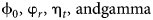 are parameters to be estimated.
Similarly, the reduced-form price equations express residential and bottled water prices in terms of the respective sets of instruments as follows:


where $p_{{\rm rt}}{\rm and\ }p_{{\rm bt}}$ are residential and bottled water prices, WGWt and WGRt denote wage rates in water treatment and food retail sectors, ELPtand RTRt represent electricity price in industrial sector and retail rents, ${\rm \zeta }_{{\rm rt}}{\rm and\ }{\rm \zeta }_{{\rm bt}}$
 reflect unobserved residential and bottled water prices, respectively, and ${\rm \lambda }_{r0}, \;{\rm \lambda }_{r1}, \;{\rm \lambda }_{r2}, \;{\rm \mu }_{rt}, \;{\rm \lambda }_{b0}, \;{\rm \lambda }_{b1}, \;{\rm \lambda }_{b2}, \;{\rm and\ }{\rm \mu }_{{\rm bt}}$
 are parameters to be estimated. We expect our price instruments to be valid, since (i) WGWt and ELPt account for residential water costs, and ${\rm WG}{\rm R}_t \ {\rm and}\ {\rm RT}{\rm R}_t$
 reflect bottled water costs and should be significantly correlated with the respective prices (i.e., relevance) and (ii) all four instruments are properly excluded from the water demand system (i.e., exogeneity).
Residential and bottled water consumption data
We base our empirical analysis of water consumption on data obtained from multiple sources. First, we compiled city-level panel data on publicly supplied water for domestic use from the U.S. Geological Survey (Dieter et al., Reference Dieter, Linsey, Caldwell, Harris, Ivahnenko, Lovelace, Maupin and Barber2018a, Reference Dieter, Maupin, Caldwell, Harris, Ivahnenko, Lovelace, Barber and Linsey2018b). The data provide information on per capita residential water consumption for 26 cities in the contiguous United States and spans two years—namely, 2010 and 2015.Footnote 3 In addition, residential water prices were collected from a city-level water price survey for the years 2010 and 2015 conducted by the Circle of Blue company. Second, bottled water price and purchase quantity data were extracted from the Nielsen Homescan data. The Nielsen Homescan data are based on self-reports from a nationally representative panel of households regarding daily food for at-home consumption that are purchased from a variety of store formats such as grocery stores, department stores, and convenience stores.Footnote 4 The data contain information on product description and characteristics, quantity purchased, expenditure and promotion, and detailed household economic and demographic characteristics. Third, we assembled city-level per capita income data from the American Community Survey, which is the largest survey conducted by the United States Census Bureau based on a sample of 3.5 million households surveyed on an annual basis (U.S. Census Bureau 2010–2015). Fourth, we obtained retail rent data from Marcus and Millichap National Retail Reports that were used to proxy food retail costs (Marcus and Millichap, 2015). Marcus and Millichap is a commercial real estate brokerage firm that also collects data on various economic and demographic aspects of real estate markets in the United States, conducts research, and publishes reports on major real estate indicators. Fifth, data on mean hourly wage of retail salespersons and mean hourly wage of water and wastewater treatment plant and system operators were gathered from the U.S. Bureau of Labor Statistics (2015). Finally, the average price of electricity was obtained from the U.S. Energy Information Administration (2010–2015).
Categorizing commodities as a combination of water type and city for two distinct years—namely, 2010 and 2015, results in 52 (i.e., 26 US cities * two years) observations for each of the residential and bottled water equations. This translates into 260 total observations for the full system of the GEASI demand, water total expenditure, and reduced-form price equations (i.e., five equations with 52 observations each). We confine our analysis to these specific cities due to limited data on supply shifters. While our sample is somewhat smaller than the household-level data used in a number of previous studies, the main advantage of the data underlying the current study is their relatively broader geographical coverage extending across all four main regions in the contiguous United States.
Table 1 presents the descriptive statistics for the main variables used in the water demand analysis. Unsurprisingly, the bulk of household water needs are typically satisfied with residential water, while the share of bottled water in total household water consumption is considerably lower. Specifically, average annual city consumption of residential and bottled water made up of 32.7 thousand and 9.4 thousand gallons, respectively. As far as the specific uses of these water types, we expect that bottled water is used for drinking (17.0 percent budget share), while residential water is mainly utilized for other household purposes (83.0 percent budget share). It can also be seen that bottled water is considerably more expensive ($2.99 per gallon) vis-à-vis residential water priced at $0.13 per gallon. Finally, the average per capita income is almost 28 thousand $US, the average of the mean hourly wage of retail salespersons and water system operators is $12.70 and $23.94, respectively, the average of the mean of the industrial electricity price is reportedly 7.61 cents/kilowatt hour, and the average rent is $19.30 per square foot.
Table 1. Descriptive statistics of the main variables

Note: Researcher(s) own analyses calculated (or derived) based in part on data from the Nielsen Company (US), LLC and marketing databases provided through the Nielsen Datasets at the Kilts Center for Marketing Data Center at The University of Chicago Booth School of Business. Total number of observations equals 52.
Estimation procedure and empirical results
We estimate the full system comprising the GEASI demand equations for residential and bottled water (equation 8), reduced-form expenditure (equation 9), as well as reduced from price equations for residential and bottled water (equations 10 and 11, respectively) via the FIML procedure. The FIML procedure is equivalent to the generalized method of moments and three-stage least squares estimation methods; however, the former is asymptotically more efficient in nonlinear models such as the one analyzed here (Hayashi Reference Hayashi2000). Our empirical framework further allows for contemporaneous correlation across the error terms of the equations in the system (8–11) and accounts for the true simultaneity between water consumption and prices (Hayashi Reference Hayashi2000).Footnote 5


where equations 8–11 are defined as before, except that the subscript g denoting city is added to emphasize the cross-section aspect of the data used.Footnote 6
Three alternative empirical specifications based on the system of equations in (8–11) are estimated to evaluate the importance of unobserved regional heterogeneity in water consumption, as well as the price and expenditure endogeneity. These specifications are as follows: (Specification a) accounts for demand interrelationship between residential and bottled water, while ignoring unobserved regional heterogeneity in consumption and price and expenditure endogeneity (based on equation 8); (Specification b) accounts for demand interrelationship between residential and bottled water, as well as unobserved regional heterogeneity in consumption, while ignoring price and expenditure endogeneity (based on equation 8); (Specification c) accounts for demand interrelationship between residential and bottled water, and unobserved regional heterogeneity in consumption, as well as addresses price and expenditure endogeneity (based on the system of equations (8–11)).
A number of different specifications of our empirical model are estimated by means of the GAUSSX programming module of Gauss platform while imposing restrictions stemming from the consumer theory (i.e., of adding-up, homogeneity, and symmetry). Furthermore, we omit the demand equation for bottled water to circumvent the singularity of the variance–covariance matrix of error terms resulting from budget shares adding-up to unity. The parameter estimates associated with the bottled water equation are recovered from the parametric restrictions of adding-up, homogeneity, and symmetry. Based on a likelihood ratio (LR) test procedure, model diagnostic test outcomes indicate that the quadratic Engel curves do not bring significant enhancement to model explanatory power (Table 2, hypothesis [i]). Furthermore, we find strong empirical evidence for precommitments in both residential and bottled water consumption (Table 2, hypothesis [ii]). Specifically, 79 percent of residential water is estimated to be due to precommitted consumption, while only 23 percent of bottled water is accounted for by precommitted demand. We also find significant unobserved regional heterogeneity in the consumption of both types of water (Table 2, hypothesis [iii]). Based on the Durbin–Wu–Hausman statistic, we may reject the null hypothesis of exogenous expenditures and prices, which makes it necessary to address both types of endogeneity (Table 2, hypothesis [iv]).
Table 2. Summary of the model diagnostic tests

Table 3 reports the GEASI demand parameter estimates along with the respective standard errors. We estimate three different specifications (i.e., a, b, c) to evaluate the effects of restrictive modeling assumptions on estimation results.Footnote 7 As is evident from Table 3, ignoring price and expenditure endogeneity, as has been done under the specifications a (ignores unobserved regional heterogeneity) and b, affects a majority of parameter estimates in both residential and bottled water demand equations. In particular, residential and bottled water price coefficients are estimated to be statistically insignificant in both equations, whereas addressing the econometric issues of expenditure and price endogeneity (specification c) leads to most parameter estimates being significant. Thus, the failure to account for the simultaneous nature of water consumption and prices on the one hand, and consumption and expenditures on the other, can bring about severe consequences and can lead to erroneous policy implications.
Table 3. Parameter estimates from the GEASI demand system

Note: These model specifications a, b, and c are as follows: (Specification a) accounts for demand interrelationship between residential and bottled water, while ignoring unobserved regional heterogeneity in consumption and price and expenditure endogeneity (based on equation 8). (Specification b) accounts for demand interrelationship between residential and bottled water, as well as unobserved regional heterogeneity in consumption, while ignoring price and expenditure endogeneity (based on the equation 8). (Specification c) accounts for demand interrelationship between residential and bottled water, and unobserved regional heterogeneity in consumption, as well as addresses price and expenditure endogeneity (based on the system of equations in (8–11)). ***, **, and * indicate statistical significance at 0.00, 0.05, and 0.10 levels of significance, respectively. Parameter standard errors are italicized and are in parenthesis. Researcher(s) own analyses calculated (or derived) based in part on data from the Nielsen Company (US), LLC and marketing databases provided through the Nielsen Datasets at the Kilts Center for Marketing Data Center at The University of Chicago Booth School of Business.
The precommitted demand parameter estimates are positive and statistically significant for both residential (0.0696) and bottled water (0.2028) (Table 3, specification c). When converted into actual gallons consumed, these estimates translate into 25.8 thousand gallons of residential water and 21.8 thousand gallons of bottled water, which account for 79 percent and 23 percent of total residential water and bottled water consumption, respectively. Interestingly, Gaudin, Griffin, and Sickles (Reference Gaudin, Griffin and Sickles2001) find that 75 percent of residential water consumption is due to precommitted demand, which is in accord with our estimate, despite the significant methodological and data differences between the two studies.
Table 4 provides the estimation results from the reduced-form price and expenditure equations. It can be seen that the parameter estimate signs are consistent with economic theory. Specifically, both water system operator wages and industrial electricity prices are estimated to have positive impacts on the residential water price (albeit the wage effect is statistically insignificant at the 5 percent significance level), which is reflective of the supply side of the price determination mechanism. Similarly, the retail wages and retail rent have positive impacts on the bottled water price. Furthermore, the share of household income allocated to water expenditures is found not to vary with rising incomes, while considerable regional heterogeneity appears to exist in water expenditures.
Table 4. Parameter estimates from the reduced-form equations and first-stage F-test outcomes
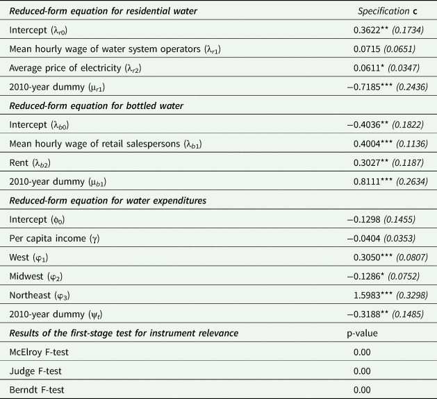
Note: ***, **, and * indicate statistical significance at 0.00, 0.05, and 0.10 levels of significance, respectively. Parameter standard errors are italicized and are in parenthesis. Researcher(s) own analyses calculated (or derived) based in part on data from the Nielsen Company (US), LLC and marketing databases provided through the Nielsen Datasets at the Kilts Center for Marketing Data Center at The University of Chicago Booth School.
To ascertain the relevance of our price and expenditure instruments, we conduct a variety of first-stage F-tests (Table 4). In contrast to single equation-based tests for a single endogenous variable, we conduct a variety of F-tests developed for a system of reduced-form equations, given the presence of three endogenous variables in our empirical framework. The results from all the tests considered provide strong empirical evidence of the relevance of the instruments used. Specifically, the p-values associated with the Berndt F-test, McElroy F-test, and Judge F-test are less than 0.00 (McElroy Reference McElroy1977; Judge et al. Reference Judge, Hill, Griffiths, Ltitkepohl and Lee1985; Berndt Reference Berndt1991). Finally, our instruments reflect the cost side of the price determination mechanism; therefore, they are properly excluded from the respective demand equations (i.e., exogeneity assumption).
Table 5 presents the GEASI-based uncompensated (Marshallian), compensated (Hicksian), and expenditure elasticity estimates evaluated at the sample mean values. The uncompensated own-price elasticities are statistically significant and conform to consumer theory. While the own-price elasticity estimate for residential water (−1.8799) is considerably elastic, one needs to bear in mind that individuals become highly sensitive to price changes only after reaching 79 percent of actual residential water consumption (i.e., precommitted quantity). Additionally, it deserves to be mentioned that finding elastic own-price elasticities in prior studies is not uncommon (e.g., Hewitt and Hanemann Reference Hewitt and Hanemann1995; Rietveld, Rouwendal, and Zwart Reference Rietveld, Rouwendal and Zwart2000; Hoffman, Worthington, and Higgs Reference Hoffman, Worthington and Higgs2006). Meanwhile, the uncompensated own-price elasticity of demand for bottled water is inelastic (−0.978), which may be partly due to a relatively small precommitted consumption (23 percent). This result is in line with the findings by Dharmasena and Capps (Reference Dharmasena and Capps2012), Dharmasena (Reference Dharmasena2010), and Zheng and Kaiser (Reference Zheng and Kaiser2008). Based on the expenditure elasticity estimates, residential water is expenditure-elastic (1.984) and bottled water is expenditure-inelastic (0.7915). Similar results are reported by Dharmasena and Capps (Reference Dharmasena and Capps2012) and Dharmasena (Reference Dharmasena2010), who also found bottled water to be expenditure-inelastic, while a number of previous studies reported positive income elasticity of demand for residential water (Nauges and Thomas Reference Nauges and Thomas2003; Martínez-Espiñeira and Nauges Reference Martínez-Espiñeira and Nauges2004; Gaudin Reference Gaudin2006; Hoffman, Worthington, and Higgs Reference Hoffman, Worthington and Higgs2006). Finally, both compensated own-price elasticities are negative and statistically significant (−1.5331 for residential water demand and −0.3248 for bottled water demand), conforming to consumer theory. We also empirically confirm that residential and bottled water are substitutes, based on the positive corresponding compensated cross-price elasticity estimates of 1.5331 and 0.3248. Of course, the extent to which tap water can be substituted for bottled water varies by city depending on a host of factors, including water quality.
Table 5. Uncompensated (Marshallian), compensated (Hicksian), and expenditure elasticity estimates from the GEASI demand model

Note: Italicized values in the parentheses are the standard errors. *, **, and *** indicate statistical significance at the 10%, 5%, and 1% levels, respectively. Researcher(s) own analyses calculated (or derived) based in part on data from the Nielsen Company (US), LLC and marketing databases provided through the Nielsen Datasets at the Kilts Center for Marketing Data Center at The University of Chicago Booth School of Business.
To evaluate the impact of ignoring price and expenditure endogeneity on the economic effects, we compute the percentage difference between the respective elasticities from the models that address and ignore price and expenditure endogeneity. As can be observed from Table 6, under these restrictive assumptions of exogeneity, expenditure elasticity for residential water is underestimated by 54 percent, while that for bottled water is overestimated by almost 16 percent. This difference is even greater for the uncompensated and compensated elasticities. For example, the uncompensated cross-price elasticity of demand between bottled and residential water is underestimated by 34.5 percent.
Table 6. Percentage difference between the elasticities from the models addressing and ignoring price and expenditure endogeneity (percent)

Note: Researcher(s) own analyses calculated (or derived) based in part on data from the Nielsen Company (US), LLC and marketing databases provided through the Nielsen Datasets at the Kilts Center for Marketing Data Center at The University of Chicago Booth School of Business.
As a final exercise, we illustrate how ignoring precommitments in water consumption, when they are present, can lead to erroneous policy implications. Specifically, water demand management policies seeking to reduce residential water usage from 32.7 thousand to say 30.0 thousand gallons annually (i.e., an 8.24 percent decrease) need to reduce residential water price by 7.74 percent in the absence of precommitments.Footnote 8 Specifically, based on the own-price elasticity formula %ΔQ res/%ΔP res = −1.0679, the targeted decrease in residential water consumption can be achieved through the following change in own price %ΔP = (0.0824/1.0679) = 0.0774, or 7.74 percent. When precommitted quantities exist, however, a considerably larger price change is required to reach the same policy objective. Specifically, following the computational steps laid out above, we find that residential water price needs to rise by 32.28 percent to yield the outcome as in the scenario when all consumption responds to price changes.Footnote 9
Concluding remarks and recommendations for future research
This study provides an empirical evaluation of the structure of demand for residential water in the United States while addressing a number of important econometric issues. Specifically, we model the demand for residential and bottled water jointly, in recognition of potential demand interdependences. Furthermore, we address simultaneity-induced water price and expenditure endogeneity by adopting a FIML procedure that accounts for the supply side of price determination mechanism. Importantly, we employ a GEASI model that is a state-of-the-art demand system that allows for potential precommitted quantities in consumption, along with unobserved consumer and region heterogeneity, and unrestricted Engle curves for both water types. Finally, our study covers a relatively large geographical area vis-à-vis the previous studies in this line of literature.
Our findings reveal a significant substitutability relationship between residential and bottled water, while substantial precommitments are established in both residential (79 percent) and bottled water (23 percent) consumption. Additionally, residential demand becomes considerably price-elastic once its precommitted level is reached. Finally, ignoring substitutability, precommitted demand, or expenditure/price endogeneity distorts the demand structure, resulting in erroneous policy implications, as illustrated in a simple exercise.
Some of the potential beneficiaries of the empirical findings stemming from this study include state regulatory agencies (public utilities commission). Specifically, these agencies can utilize our findings in their efforts to regulate residential water supply operators (who act as natural monopolies) in a way that ensures that the public interest is protected. Our estimated precommitted water consumption provides particularly valuable information to water supply operators from the perspective of designing accurate and effective pricing strategies. Additionally, a better understanding of the water demand structure can assist water supply operators in predicting the amount of revenue necessary to pay for capital investments used in the upkeep and improvement of the water supply infrastructure. Finally, estimated demand elasticities can be used by policymakers to simulate and evaluate the effects of tax and water conservation policies (e.g., a rather high level of 79 percent of precommitted residential water demand suggests that non-price-based policies will be relatively more effective than price-based policies in terms of achieving residential water conservation targets).
A few recommendations for future research are worth mentioning. First, future research would benefit from extending the analysis by including city-level demographic information, assuming that the number of observations is sufficiently large. Second, since the residential water consumption data are only reported once every five years, it will be worthwhile for future research to incorporate more years as they become available. Finally, future research would benefit significantly from more disaggregate data on household-level water consumption as such data become available. This would also make it possible to investigate the differential impacts of block- and flat-rate prices.
Data availability statement
This research was conducted based on Nielsen proprietary data; therefore, data cannot be made public.
Acknowledgements
Researcher(s)’ own analyses calculated (or derived) based in part on (i) retail measurement/consumer data from Nielsen Consumer LLC (“NielsenIQ”); (ii) media data from The Nielsen Company (US), LLC (“Nielsen”); and (iii) marketing databases provided through the respective NielsenIQ and the Nielsen Datasets at the Kilts Center for Marketing Data Center at The University of Chicago Booth School of Business. The conclusions drawn from the Nielsen data are those of the researcher(s) and do not reflect the views of NielsenIQ or Nielsen. Neither NielsenIQ nor Nielsen is responsible for, had any role in, or was involved in analyzing and preparing the results reported herein.
Funding statement
This research received no specific grant from any funding agency, commercial, or not-for-profit sectors.
Conflicts of interest
The author(s) declare none.


 Open access