


I. INTRODUCTION
One of the most important key factors of display performance is the contrast ratio, which represents the ratio between how dark or bright the display can get. In general, the dynamic range refers to the ratio between the brightest whites and the darkest blacks given at the same time in a specific image or video frame. The dynamic range is often measured in “stops,” which is the logarithm base-2 of the contrast ratio. While conventional display technology is capable to reach brightness ranges from 1 to 300 cd/m2 (nits) and 8 stops of dynamic range, objects captured in sunlight can easily have brightness values up to 10 000 nits. Considering that the human eye can see 14 stops of dynamic range in a single view; clearly, conventional display technology is unable to show luminance-realistic images.
Images associated to display technology with narrow dynamic range and a low brightness have been retroactively called Low Dynamic Range (LDR) images. A High Dynamic Range (HDR) image refers to an image that encodes a higher dynamic range and a larger amount of brightness than a reference LDR image. To improve the dynamic range of a display, manufacturers have innovated in the development of new display technologies. Recent developments have yielded LED displays, which contain an array of independently controlled high-power white LEDs as backlighting system, which allows reaching a peak brightness of 6000 nits and 14 stops of dynamic range [1]. Despite LED displays offer the best alternative for manufacturers to design HDR displays, OLED technology also has been used for this purpose. LED technology tolerates higher peak brightness (more than 1000 nits) and higher black levels (less than 0.05 nits). OLED technologies tolerate lower brightness (less than 1000 nits) and deeper black levels (less than 0.0005 nits). In general, LED technology allows manufacturers to create displays with high peak brightness levels but less deep blacks, while OLED technology allows them to build displays with lower peak brightness but deeper blacks. Additionally, in order to represent a wide dynamic range in an image, the number of bits for its representation needs to be increased. Hence, a wider range of luminance levels can be encoded to display images with a larger dynamic range.
HDR imaging overcomes the dynamic range limitations of traditional LDR imaging by capturing the full range of the visible light spectrum and colors that exist in the real world by performing operations at high bit-depths [Reference Chalmers, Karr, Suma and Debattista2]. Hence, HDR technology is capable of enhancing the quality of television experience with a dynamic range compared to the Human Visual System (HVS) [Reference Zhang, Reinhard and Bull3]. Additionally, due to its truthful representation of the real world with more details and information about the scenes, it is becoming more relevant for other fields such as video game development, medical imaging, computer vision, scientific visualization, surveillance, among others [Reference Dong, Pourazad and Nasiopoulos4].
Unfortunately, a large amount of existing video content has already been recorded and/or graded in LDR. To display LDR content on HDR displays, an inverse/reverse tone mapping algorithm is required. Inverse tone mapping algorithms work on reproducing real-world appearance HDR images by using LDR images as input [Reference Reinhard, Heidrich, Debevec, Pattanaik, Ward and Myszkowski5, Reference Wang6]. Different techniques have been proposed in the past few years, each of them addresses the problem of inverse tone mapping in a different way. Common limitations of these techniques are (1) they need human intervention to decide the most suitable parameters to use for the inverse tone mapping, (2) they are limited to produce HDR images with a limited peak brightness (between 1000 and 3000 nits), (3) they are designed to preserve the appearance of the original LDR image without considering the artistic intentions inherent to the HDR domain (like deep shadows and bright highlights), and (4) they are complex and their computation times are so high that they are not suitable for practical purposes such as real-time inverse tone mapping or being embedded on hardware with limited resources.
In this article, as an extension of our previous work [Reference Luzardo, Aelterman, Luong, Philips, Ochoa and Rousseaux7], we describe a fully-automatic inverse tone mapping algorithm based on dynamic mid-level mapping. We carried out an extensive objective evaluation of our algorithm against the most recent methods of inverse tone mapping in the literature. Additionally, we conducted a subjective pair-wise comparison experiment in order to validate our previous findings. This paper is organized as follows: an overview of previous works is given in Section II. Then, the proposed expansion function and the inverse tone mapping algorithm are described in Section III and Section IV, respectively Experimental results are presented in Section V. Finally, concluding remarks are discussed in Section VI.
II. RELATED WORK
Several methods for inverse tone mapping have been proposed in recent years. These can be grouped according to how the dynamic range expansion problem is tackled [Reference Banterle, Artusi, Debattista and Chalmers8]:
• Global operators. Where the same global expansion function is applied to each pixel of the LDR image. A monotonic function is usually adopted and its shape is adjusted according to the characteristics of the scene present in the image. Typical characteristics are the scene type (dark, average, bright), contrast, amount of saturated pixel, mean and median luminance, and the perceived amount of brightness in the scene [Reference Luzardo, Aelterman, Luong, Philips, Ochoa and Rousseaux7, Reference Bist, Cozot, Madec and Ducloux9–Reference Masia, Serrano and Gutierrez11].
• Local operators. Where each region of the image is expanded in a different way, depending on a given criterion. Commonly, these methods classify different parts of the image as a region with a diffuse or a specular highlight in order to expand each one using a different expansion function. Other methods seek to identify salient objects in the image in order to expand them in a different way than in the rest of the image [Reference Wang6, Reference Huo, Yang and Li12, Reference Masia and Gutierrez13].
• Expansion maps. Where an expansion map is used to direct the expansion of the LDR content. This expansion map is a non-binary mask that represents the weights to be used for the expansion of each pixel in the LDR image. The main difference of each method is the way how this map is created [Reference Banterle, Ledda, Debattista and Chalmers14–Reference Kovaleski and Oliveira17].
• User-guided techniques. Where the user intervention is required to address the expansion. In these methods, the user helps to add detailed information lost in over/under-exposed areas on the original LDR image prior to being expanded [Reference Wang, Wei, Zhou, Guo and Shum18].
• Deep Learning techniques. Where Deep Convolutional Neural Networks (CNNs) are used to automatically expand an input LDR image. Not all, but most of these methods address the dynamic range expansion in to reconstruct data that have been lost from the original signal due to clipping, quantization, tone mapping, or gamma correction [Reference Eilertsen, Kronander, Denes, Mantiuk and Unger19–Reference Zhang and Lalonde24].
In the remainder of this section, we discuss some very specific inverse tone mapping techniques. Kovaleski and Oliveira [Reference Kovaleski and Oliveira17] proposed a reverse tone mapping operator for images and videos which can deal with images with a wide range of exposure conditions. This technique is based on the automatic computation of a brightness enhancement function, also called expand-map, that determines areas where image information may have been lost and fills these regions using a smooth function. Likewise, Huo et al. [Reference Huo, Yang, Dong and Brost15] proposed a method that considers the perceptual properties of the Human Visual System (HVS). Their approach is based on the fact that the perceived brightness of each point in an image is not determined by its absolute luminance, but by a complex sequence of steps that happens in the HVS. According to the authors, due to this and the fact that for applications of rendering a believable HDR impression (entertainment/TV) rather than a scientifically HDR recovery, it is not necessary to create a perfect reconstruction of the original HDR image. Rather, an approximation that does not produce a significant change in the visual sensation experienced by the observers should be enough, which can be achieved by imitating the local retina response. Their algorithm first extracts the luminance and chrominance channels from the LDR input image. Then, the luminance channel is used to compute the local surrounding luminance using an iterative bilateral filter. Afterward, the new expanded HDR luminance is obtained by combining the input luminance channel and the local surrounding using the local response of retina as the mathematical model, which was estimated previously from the global one. Finally, the HDR image is generated by combining the computed HDR luminance and the chrominance channel from the input LDR image. According to the authors, this method is capable to enhance the local contrast and preserve details in the resulting expanded HDR image.
Masia et al. [Reference Masia, Serrano and Gutierrez11] proposed a dynamic inverse tone mapping algorithm based on image statistics. The main assumption of this method is that input LDR images are not always correctly exposed. In this way, the authors propose to use a simple gamma curve as inverse tone mapping operator in which the gamma value is estimated from a multi-linear model that incorporates the key value [Reference Akyuz and Reinhard25], the number of overexposed pixels, and the geometric mean luminance as input parameters. Bist et al. [Reference Bist, Cozot, Madec and Ducloux9] proposed a method based on the conservation of the lighting style aesthetics. As with previous approaches, this method uses a simple gamma correction curve as an expansion operator; however, in this method, the gamma value is computed based on the median of the luminance in the input LDR image. Despite these methods produce good results across a wide range of exposure conditions; because they are based on preserving the aspect of the original LDR image, they might not always reflect the artistic intentions intrinsic to the HDR domain.
In recent studies, Endo et al. [Reference Endo, Kanamori and Mitani21] proposed an inverse tone mapping method based on Deep Learning. This is one of the first approaches that explore the use of deep CNNs. The key idea is to synthesize LDR images taken with different exposures based on supervised learning, and then reconstruct an HDR image by merging them. In a so-called learning phase, authors trained two deep neural network models by using 2D convolutional and 3D deconvolutional networks to learn the changes in exposures of the synthesized LDR images created from an HDR dataset. The first model was trained to output N up-exposure images, while the second one to output N down-exposed images. Both models were built using the same architecture but trained separately. The synthesized images used to train the models were created by simulating cameras with different camera response functions and exposures from each image in the HDR dataset. For the inverse tone mapping of a single input LDR image; first, a set of synthesized LDR images is generated using the built models, in a so-called inference phase. Then, the input LDR image and k synthesized LDR images selected systematically, s.t. $k\leq 2N$ , are used to compute the final HDR image by merging them using the method proposed by Debevec and Malik [Reference Debevec and Malik26]. According to the authors, their method can reproduce not only natural tones without introducing visible noise but also the colors of saturated pixels. Likewise, Eilertsen et al. [Reference Eilertsen, Kronander, Denes, Mantiuk and Unger19] proposed a technique for HDR image reconstruction from a single exposure using deep CNNs. This method is focused on reconstructing the information that has been lost in saturated image areas, such as highlights lost due to saturation of the camera sensor, by using deep CNNs. The authors first trained the model using a dataset of HDR images with their corresponding LDR images. This dataset was generated by simulating sensor saturation for a range of cameras using random values for exposure, white balance, noise level, and camera curve. The model proposed by the authors for the HDR reconstruction is a fully convolutional deep hybrid dynamic range autoencoder network. It is defined as “hybrid” because it mixes the behavior of a classic autoencoder/decoder that transforms and reconstructs dimensional data, and a denoising autoencoder/decoder that is trained to reconstruct the original uncorrupted data. The encoder operates on the LDR input image, which contains corrupted data in saturated regions, to convert it into a latent feature representation. Then, the decoder uses this representation to generate the final HDR image by restoring corrupted data. Authors claim that their method can reconstruct a high-resolution visually convincing HDR image using only an arbitrary single exposed LDR image as an input.
In this paper, we propose a fully-automatic inverse tone mapping algorithm based on mid-level mapping. Our approach allows expanding LDR images into HDR domain with peak brightness over 1000 nits. For this, a computationally simple non-linear expansion function that takes only one parameter is used. This parameter is automatically estimated using simple first-order image statistics. Unlike [Reference Bist, Cozot, Madec and Ducloux9, Reference Masia, Serrano and Gutierrez11], our proposed expansion function offers better capabilities to increase the perceived image quality of the resulting HDR image than a gamma expansion curve. Furthermore, it can expand an LDR image into an HDR image with a peak brightness of over 1000 nits. The proposed algorithm can reach the same performance of more computationally complex methods, with the advantage that it is simple enough to be used for practical purposes such as real-time processing in embedded systems.
III. PROPOSED EXPANSION FUNCTION
To expand the dynamic range of an LDR image ($I_{LDR}$ ) and obtain its inverse tone-mapped HDR image counterpart ($I_{HDR}$
 ), a method based on mid-level mapping is proposed. The tone mapper function proposed in [Reference Lottes27] is adopted. In this function, two parameters to control the shape of the curve (a and d) and two parameters to set the anchor point are defined (b and c), as follows:

Where L is the display luminance of $I_{LDR}$ , $L_w$
 is the expanded luminance of $I_{HDR}$
 in the real-world domain, and $L_w\in [0,L_{w,\max }]$
 . The parameter $L_{w,\max }$
 is the maximum luminance in which $I_{LDR}$
 wants to be expanded, and its value usually depends on the peak brightness of the HDR display where $I_{HDR}$
 will be displayed. $L_{w,\max }$
 can also be considered as the relative luminance to the maximum luminance produced by the HDR display. Then, a value of 1 means that an output HDR-image that reaches the peak luminance of the HDR display is required.
As mentioned by the authors, this function was designed to result in believably real images and to allow adaptation to a large range of viewing conditions. In our case, this formulation offers sufficient freedom to change the overall brightness impression of the scene and preserve its artistic intent, without resulting in an “unbelievable” image.
Figure 1 shows a graph of the proposed function. The parameters a and d allow controlling the shape of the so-called toe (contrast) and shoulder (expansion speed) of the curve, respectively. Our function offers the possibility to fine-tune the resulting inverse tone-mapped HDR image to improve its perceived image quality, for example by increasing the contrast [Reference Rempel28]. As can be seen in Fig. 1, the parameters $m_{i}$ and $m_{o}$
 act as an anchor point for the curve and represent the middle-gray value defined for the input $I_{LDR}$
 and the expected middle-gray value in the output $I_{HDR}$
 , respectively. The middle-gray value is a tone that is perceptually about halfway between black and white on a lightness scale. These parameters enable us to control the overall luminance of $I_{HDR}$
 . For this, the parameter $m_{i}$
 is set to the middle-gray predefined for $I_{LDR}$
 (e.g. 0.214 for sRGB linear LDR images), and $m_{o}$
 is adjusted to the middle-gray value desired in $I_{HDR}$
 . In practice, this operation can be seen as mid-level mapping. A low value for the $m_{o}$
 causes $I_{HDR}$
 to become darker, and a higher value brighter.

Fig. 1. The shape of the proposed inverse tone mapping function. LDR input values are normalized between 0 and 1. The maximum output HDR value depends on the peak luminance in nits of the HDR display e.g. 6000, or 1 for expressing that we intend to achieve the maximum luminance supported by the display.
Considering the following constraints: $f(m_{i})=m_{o}$ and $f(1)=L_{w,\max }$
 . The anchor points b and c can be computed as follows:


Note that practically these conditions imply that $m_i$ should be different from 0 (a completely black frame) and 1 (a completely white frame), both are border cases that can easily be accounted for.
As can be seen, the proposed function in equation (1) is applied only to the luminance channel in order to leave the chromatic channels of $I_{LDR}$ unaffected. Despite the existence of other methods that allow reconstructing the color image while preserving its saturation better [Reference Artusi, Pouli, Banterle and Akyüz29], we decided to use the method proposed by Mantiuk et al. [Reference Mantiuk, Tomaszewska and Heidrich30]. In this, the color image $I_{HDR}$
 is reconstructed by preserving the ratio between the red, green, and blue channels as follows:

Where $C_{LDR}$ and $C_{HDR}$
 denote one of the color channel values (red, green, blue) of the $I_{LDR}$
 and $I_{HDR}$
 , respectively. The parameter s is a color saturation parameter and allows to compensate for the loss of saturation during the luminance expansion operation. By fixing the saturation (s), contrast (a), and expansion speed (d), the expand operation of $I_{LDR}$
 can be performed easily using equations (1)–(4). In addition, the proposed function allows changing the peak brightness of the resulting HDR image without affecting its middle tones, which is controlled by the parameter $m_o$
 .
.
IV. FULLY-AUTOMATIC INVERSE TONE MAPPING
The proposed solution exploits the premise that an inverse tone mapping procedure should take into account the context in which the scene unfolds [Reference Akyüz, Fleming, Riecke, Reinhard and Bülthoff31]. In this sense, the context could be objectively expressed as features of the scene that are used to lead the inverse tone mapping process.
Our algorithm is based on a mid-level mapping approach. Image features are used to estimate the middle-gray level of the HDR output. For the proposed expansion function, parameters s, a, and d are fixed manually; then, the input $m_o$ , the value required for the expansion operation, is automatically estimated through a multi-linear function. Our function uses simple image-statistics from the LDR image as input parameters to estimate $m_o$
 . Section (A) describes the scene image dataset used for training, Section (B) explains how the corresponding human-chosen inverse tone mapping parameters were obtained through psycho-visual experiment, and Section (C) describes the machine learning method (multi-linear regression) used to estimate the inverse tone mapping parameters from scene features.
A) HDR-LDR Image Dataset
The following HDR video datasets were used to create our HDR-LDR Image Dataset: Tears of Steel [32] (1 video sequence), Stuttgart HDR image dataset [Reference Froehlich, Grandinetti, Eberhardt, Walter, Schilling and Brendel33] (15 video sequences), and a short film (1 video sequence) created by the Flemish Radio and Television Broadcasting Organization (VRT). These video datasets were selected because they include video sequences that contain scenes with a wide range of contrast and lighting conditions. Additionally, they were professionally graded by experts from VRT in HDR and LDR, using a SIM2-HDR47E HDR screen [1] and a Barco type RHDM-2301 LDR screen as reference displays, respectively. Professionally graded video content refers to video sequences that have been obtained by altering and/or enhancing a master (or a raw input video) in order to be properly displayed on a specific display. This process involves an artistic step, where the “grader” manipulates the input to better express the director's artistic intentions on the final graded content, which is extremely important to offer a reliable base to the discussion on how the content is perceived by the viewers.
From each video sequence in the HDR video datasets, we obtained two professionally graded video sequences, one in LDR and another one in HDR. HDR video sequences obtained are considered as ground truth, with most of the artistic intentions that content creators consider when they work in the HDR domain. The HDR-LDR Image Dataset was created by selecting one frame per second from each professionally graded video sequence. As can be seen in Table 1, the entire dataset includes 1631 pairs of images, an LDR image and its HDR counterpart. More details about the image dataset created for this study can be seen in Table 1. Figure 2 shows examples of LDR images from the dataset.

Fig. 2. Example of LDR images obtained from the HDR-LDR image dataset. As can be seen, the dataset contains images with a wide range of contrast and lighting conditions.
Table 1. Details about the size and number of pairs included in the HDR-LDR Image Dataset.

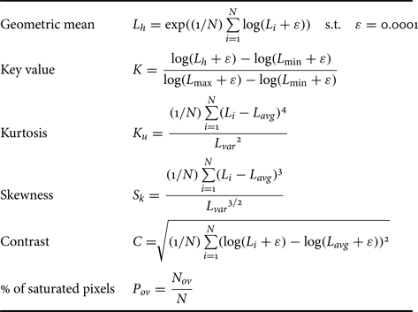
For each LDR image in the dataset, simple first-order image statistics, most of them computed on the luminance (L), were extracted. Image statistics include the average (${L_{avg}}$ ), variance (${L_{var}}$
 ), and median (${L_{med}}$
 ), and those included in Table 2. Images in the dataset were normalized into the $[0,1]$
 range and linearized by using a gamma correction curve with a power coefficient value $\alpha =2.2$
 , hence L was computed as follows:

Where R, G, and B are, respectively, the red, green, and blue channel of the linearized input image. In Table 2, ${L_{\min }}$ and ${L_{\max }}$
 refer to the minimum and maximum luminance value, respectively. ${N}$
 is the total number of pixels in the image without outliers, and ${N_{ov}}$
 is the total number of overexposed pixels. Overexposed pixels refers to those pixels where at least one color channel is greater than or equal to $(254/255)$
 . The contrast ${C}$
 was computed using only the luminance channel in logarithmic scale.
Table 2. First-order image statistics computed.
B) Subjective study
To carry out our subjective study, we selected a subset of 180 pairs of images (an LDR and its HDR image counterpart) from the HDR-LDR Image Dataset, which corresponds to 11% of the total number of pairs in the dataset. These pairs were selectively chosen in such a way the final subset contains images with equally distributed contrast and lighting conditions.
Six different middle-gray values ($m_o$ ) to inverse tone map each LDR image from the subset were obtained. Six non-experts participants, between 25 and 40 years old with normal eye-sight, took part in this study. They were asked to tweak $m_o$
 until they found the subjective best match between the inverse tone-mapped HDR image and its corresponding professionally graded HDR image (ground truth).
To facilitate the matching task and prevent that the differences in saturation between the two images affect our results, both, the luminance channel of the inverse tone-mapped image ($L_{EDR}$ ) and the luminance channel of HDR ground truth ($L_{HDR}$
 ), were displayed on the same display, a SIM2 HDR screen, in a four split-screen pattern. Figure 3 depicts how the subjective study to obtain $m_o$
 was carried out.
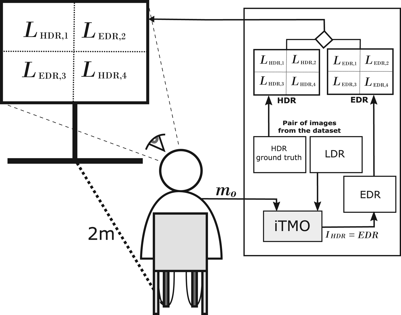
Fig. 3. Scheme of the subjective experiment carried out to manually obtain middle-gray out values that best match the luminance channel of the inverse tone-mapped HDR image (EDR) and its corresponding professionally graded HDR image (HDR) in the pair. The middle-gray value ($m_o$ ) is used by the inverse tone mapping algorithm (iTMO) to compute EDR.
As can be seen in Fig. 3, $L_{EDR}$ and $L_{HDR}$
 were divided into four regions. The top-left and bottom-right regions of $L_{HDR}$
 ($L_{HDR,1}$
 and $L_{HDR,4}$
 ) and the top-right and bottom-left regions of $L_{EDR}$
 ($L_{EDR,2}$
 and $L_{EDR,3}$
 ) were selected and displayed on the HDR screen. A desktop application was implemented to collect the middle-gray values from the participants. In this, the participant sits 2 m from the screen changed the $m_o$
 value using a slider-like control. This value was used as an input parameter to compute $L_{EDR}$
 in real-time using the $m_o$
 value selected by the participant. For this study, the contrast (a) and expansion speed (d) were set manually in 1.25 and 4.0, respectively, in order to increase the contrast and minimize that diffuse whites in the input produce artifacts in the output. Similarly, the saturation (s) was manually fixed in 1.25 as suggested in [Reference Bist, Cozot, Madec and Ducloux9], and ${L_{w,\max }}$
 in 0.67 to specify that we want to reach only 67% of the maximum luminance of the SIM2 display (around 4000 nits). A total of 1080 $m_o$
 values (180 values per participant) were collected. To avoid any light interference, this study was conducted in a light-controlled room with dim lights.
C) Multi-linear regression
As is [Reference Masia, Serrano and Gutierrez11], a multi-linear regression approach was used. We seek to model the relationship between the middle-gray value in the output ($m_o$ , dependent variable) from first-order image statistics (independent variables). This allowed us to keep the model simple enough in order to have the possibility of running the proposed inverse tone mapping algorithm in real-time.
First of all, an outlier analysis was performed over the data collected in the subjective study. In this analysis, all observations that were deemed as extreme values were removed. Given the IQR (Interquartile Range) of the samples in a group (values of $m_o$ obtained for the same pair of images), an extreme value is a data point that is below $Q_1-1.5IQR$
 or above $Q_3+1.5IQR$
 . Then, a multivariate outliers detection using Mahalanobis' distance was performed [Reference Filzmoser, Garrett and Reimann34]. Mahalanobis was used as a metric for estimating how far each case is from the center of all the variables' distributions. At the end of the outlier analysis, 47 input values were removed from the dataset. Consequently, a multi-linear regression was carried out using a step-wise regression method for variable selection. In this method, a variable is entered into the model whether the significance level of its F-value is less than a so-called entry value, and it is removed if the significance level is greater than the removal value. For this, values of 0.05 and 0.10 were used as entry and removal value. After we applied this method, the following multi-linear model was obtained:

The P-value obtained for the F-test of overall significance test was much lower than our significance level ($F(3,126.673)$ , p<0.01). This test is a specific form of the F-test that compares a model with no predictors to the model obtained in the regression. It also contains the null hypothesis that the model explains zero variance in the dependent variable [Reference Draper and Smith35]. Then the lower P-value obtained means that the model explains a significant amount of the variance in the middle-gray output value ($m_o$
 ). In other words, we can conclude that the linear combination of the geometric mean ($L_h$
 ), contrast ($c_o$
 ), and the percentage of overexposed pixels ($P_{ov}$
 ) were significantly related to the middle-gray output value ($m_o$
 ).
).
We also found that the $R^2$ of our model was 0.702 ($R^2=0.702$
 ). $R^2$
 is a statistical measure of how much of the variability in the outcome is explained by the independent variables [Reference Draper and Smith35]. This means that the 70% of the variation in the linear combination of the geometric mean ($L_h$
 ), contrast ($C$
 ), and the percentage of overexposed pixels ($P_{ov}$
 ), is explained by the equation (6).
As can be seen in equation (6) and as was expected, the geometric mean (${L_h}$ ), which is the parameter that represents the perceptual overall brightness of the input image, has the highest positive relation with the middle-gray value in the output ($m_o$
 ), followed by the contrast (${C}$
 ). This means that LDR images with a high perceptual brightness value tend to expand into HDR images with high brightness. This is also controlled by the contrast, in the sense that LDR images with high perceptual brightness but with lower contrast are not expanded to very bright HDR images. Another interesting finding was that the negative relation between the percentage of overexposed pixels (${P_{ov}}$
 ) and $m_o$
 acts as a control parameter that avoids that an overexposed image to be expanded to a very bright HDR image. In fact, in the presence of a highly overexposed image, ${C}$
 has a value close to zero, and ${L_h}$
 and ${L_h}$
 close to one. This results in a dimmed positive middle-gray output value ($m_o$
 ) which is a more pleasant inverse tone-mapped HDR image.
It should be noted that equation (6) produces acceptable results for natural scenes. During an extensive testing and after a detailed analysis, it was verified that equation (6) only degenerates in very rare cases: artificial (non-natural) frames that are made up nearly completely (>98%) of monochromatic blue pixels that are overexposed.
V. RESULTS
We intend to show that the proposed method is qualitatively in the same league as the state-of-the-art methods. To prove this, we use “ground truth” data, i.e. video frames of which both an HDR and LDR graded version are available. We intend to measure how close the LDR-to-HDR converted content is to the actual HDR-graded versions mainly using full-reference metrics. Two different quality metrics were used: Calibrated Method for Objective Quality Prediction (HDR-VDP-2.2) [Reference Narwaria, Mantiuk, Da Silva and Le Callet36] as the main full-reference quality metric and Dynamic Range Independent Image Quality Assessment (DRIM) [Reference Aydin, Mantiuk, Myszkowski and Seidel37].
HDR-VDP-2.2 is a visual metric that compares a pair of images, a reference and a test image, usually with the same dynamic range. This metric provides a so-called Probability of Detection Map (PMap) that describes the probabilities of detection of differences between both images at each pixel point, which is related to the perceived quality. A higher detection probability implies a higher distortion level at the specific pixel. HDR-VDP-2.2 also provides a measurement of quality with respect to the reference image expressed as a mean-opinion-score or simply Q-score. Likewise, DRIM is a full-reference quality metric that is used to compare a pair of images regardless of their dynamic ranges. This metric generates a so-called Distortion Map, which represents the visible structural changes to the human eye between a reference and a test image. In this map, three classes of structural changes are described: loss of visible contrast (LVC), amplification of invisible contrast (AIC), and reversal of visible contrast (RVC).
The proposed method was compared with the most recent inverse tone mapping approaches that have been listed in Table 3. For this assessment, we created a test dataset composed of images from the HDR-LDR image dataset that were not included in the subjective study to derive the equation (6). Additionally, we included 10 pairs of images from the DML-HDR dataset [Reference Banitalebi-Dehkordi, Azimi, Pourazad and Nasiopoulos38]. It should be noted that the images from the DML-HDR dataset were not professionally graded. The HDR images from the DML-HDR dataset were tone-mapped using the Mantiuk et al. [Reference Mantiuk, Daly and Kerofsky39] operator to obtain the LDR images counterpart. In this evaluation, LDR images from the final test dataset were used as input for the assessed inverse tone-mapping algorithms and HDR images were considered as the ground truth.
Table 3. Inverse Tone Mapping Algorithms used for the comparison.
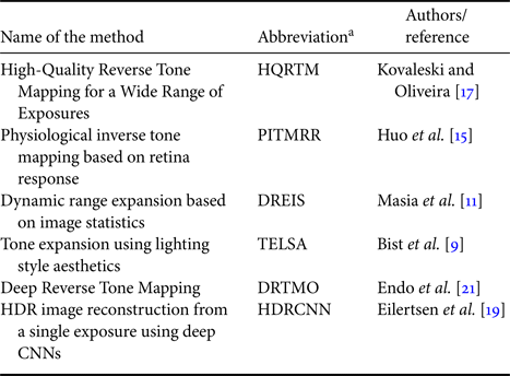
aThese abbreviations will be used to refer these methods in the document.
HDR-VDP-2.2 allowed us to compare an inverse tone-mapped HDR image (EDR) using the HDR image ground truth (HDR) as a reference. Each LDR image (LDR) from the test dataset was inverse tone-mapped using the proposed method and methods listed in Table 3 to compute the inverse tone-mapped HDR images to be tested. Default parameter values recommended by the authors were used for inverse tone mapping. The inverse tone-mapped HDR images obtained by each method were evaluated using HDR-VDP-2.2. The software available at [Reference Mantiuk, Kim, Rempel and Heidrich40] and the following parameters were used for the evaluation: absolute luminance comparison, automatic computation of the pixels per degree, 1920 horizontal display resolution, 1080 vertical display resolution, 47 inches display diagonal size, and viewing distance equal to 1 m. The outputs from DRTMO and HDRCNN were scaled to 1000 nits and calibrated using the SIM2 display.
Figure 4 shows some Probability of Detection Maps generated by HDR-VDP-2.2. Red color represents those pixels with a high probability that an average observer will notice a difference between HDR and EDR. Probability Detection Maps obtained in this evaluation are included in the Supplementary material. Figures 5 and 6 show the Mean Q-score obtained by HDR-VDP-2.2. The last one shows the results grouped according to which video sequence of the processed image of the test dataset belongs to.
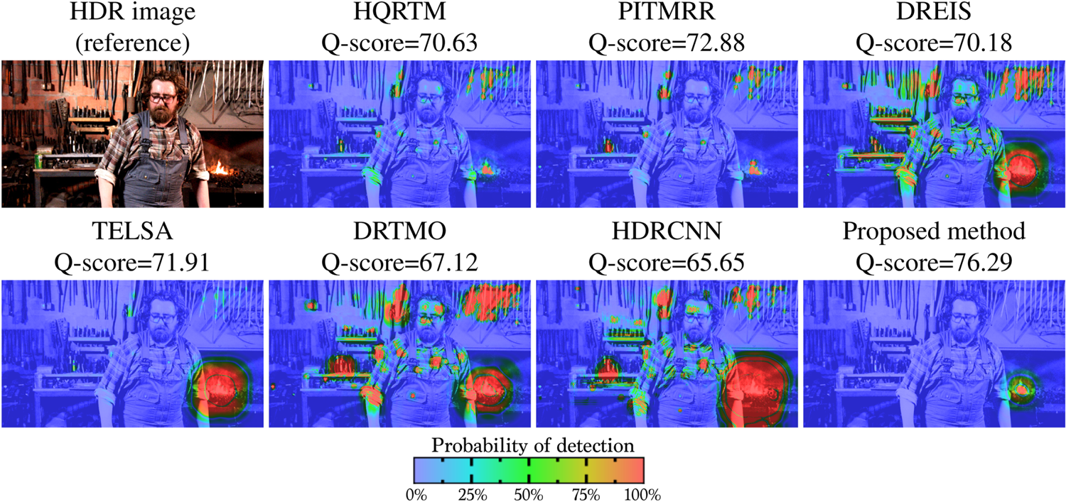
Fig. 4. Example of maps generated by HDR-VDP-2.2. The Quality Score (Q-score) is shown on the top of each map.

Fig. 5. Mean Q-scores obtained by HDR-VDP-2.2. Error bars represent the 95% confidence intervals. Horizontal lines represent homogeneous subsets from post-hoc comparisons using the Tukey HSD test.

Fig. 6. Mean Q-scores obtained by HDR-VDP-2.2. Results have been grouped according to which sequence the processed image of the test dataset belongs to. Error bars represent the standard deviation.
As can be seen in Figs 5 and 6, the proposed method together with DRTMO produce on average better Q-score results in comparison with the other assessed methods (except for the images that belong to DLM-HDR). It should be noted that, although our proposed method is far less complex than DRTMO, it can produce on average similar Q-score results. These results were further analyzed for significance using Kruskal–Wallis one-way ANOVA followed by Tukey Dunn post-hoc test because the data did not fit the assumptions of an ANOVA. This analysis, allowed us to identify which methods produced results that were driving different mean Q-scores. In Fig. 5, error bars represent a 95% confidence interval and the horizontal lines the homogeneous subset from post-hoc comparisons using the Tukey Dunn post-hoc test.
In Fig. 5, it may also be noted that DREIS ($70.56\pm 6.02$ ), PITMRR ($70.69\pm 5.23$
 ), TELSA ($70.75\pm 6.68$
 ), and HQRTM ($71.18\pm 5.87$
 ) show similar results in mean Q-scores; more specifically, they do not show a statistically significant difference in mean Q-scores among them. Results in mean Q-scores obtained by DRTMO ($74.61\pm 5.40$
 ) and the proposed method ($73.97\pm 6.54$
 ) are the better scored. We found that their differences in mean Q-scores were statistically significant with respect to the results obtained by the other methods and they do not show a statistically significant difference between them. Finally, we found that HDR images from HDRCNN ($68.83\pm 6.32$
 ) yield the lowest mean Q-scores and show a statistically significant difference in mean Q-scores with respect to the other assessed methods.
Likewise, inverse tone-mapped HDR images obtained by each method were visually inspected, and it was observed that even though HDRCNN can better reconstruct information lost in saturated areas, their results differ most from the HDR reference. Figure 7 shows the resulting inverse tone-mapped HDR image obtained by each method that contains details in saturated areas not present in the input LDR image (flame and iron-bar). As can be seen, for this scene HDRCNN better reconstructs the information lost in these areas in comparison with the other methods; however, the overall brightness is higher than the HDR reference. Likewise, as can be seen in Fig. 7, DRTMO occasionally produces artifacts on the reconstructed saturated areas (flame).

Fig. 7. Comparison of different results of inverse tone mapping. An image with a lack of details in saturated areas was used as input. DRTMO and HDRCNN better reconstruct the lost details. Q-score is shown in parentheses. HDR images were tone-mapped by Mantiuk et al. [Reference Mantiuk, Daly and Kerofsky39] operator.
As mentioned before, we also compared the inverse tone-mapped images obtained by using the proposed method with those obtained by the methods listed in Table 3 using DRIM as a quality metric. This time, only a small random sample of 147 images from the test dataset was used. This was decided due to the fact that DRIM does not provide the source code that allows testing a large number of images, but only a web site where each image must be uploaded one by one. DRIM allowed us to objectively compare the inverse tone-mapped HDR images with the LDR input images in terms of structural changes. These structural changes are represented with different colors on the distortion map generated by this metric. Green color, red color, and blue color are used to represent lost of visible contrast (LVC), amplification of invisible contrast (AIC), and reversal of visible contrast (RVC), respectively. For this evaluation, the online software available at [Reference Aydin, Mantiuk, Myszkowski and Seidel41] with the following parameters was used: automatic computation of the pixels per degree, 1920 horizontal display resolution, 1080 vertical display resolution, 47 inches display diagonal size, and a viewing distance equal to 0.5 m, and 0.0025 peak contrast.
Distortion maps obtained by DRIM revealed that the proposed method causes far less RVC and LVC, and much more AIC than the other tested methods. All these characteristics help to increase the perceived quality of our method. The presence of a high AIC indicates that our algorithm can better disclose/enhance some details that are not present in the original LDR image and in this way it contributes to the quality of the resulting inverse tone-mapped HDR image. In general, for an inverse tone mapping operator, loss and reversal of visible contrast are undesirable results, while amplification of invisible contrast tends to increase perceived image quality [Reference Huo, Yang, Dong and Brost15, Reference Kovaleski and Oliveira17, Reference Rempel28, Reference Huo, Yang and Brost42].
Figure 8 shows examples of distortion maps obtained in this assessment. As can be seen, DRIM provides a pixel-wise distortion map. The saturation of each color (red, blue, or green) in the distortion map indicates the magnitude of the detection probability that can be seen as the magnitude of perceived distortion. More distortion maps obtained in this evaluation are included in the Supplementary material.

Fig. 8. Distortion maps generated by DRIM.
Additionally, we visually inspected the results obtained using highly overexposed images from the dataset as input. Figure 9 shows results obtained by each algorithm and our proposed solution. As can be seen, our method does not produce results with unnatural appearances when process highly overexposed natural images. However, DRTMO and HDRCNN produce artifacts in overexposed areas. It was found that the only degenerate cases in our method are artificial (non-natural) scenes that consist of more than 98% of overexposed, monochromatic blue pixels.

Fig. 9. Comparison of different results obtained by each tested algorithm using a highly overexposed image as input. As can be seen, DRTMO and HDRCNN produce artifacts in overexposed areas. For visualization, HDR images were tone-mapped by Mantiuk et al. [Reference Mantiuk, Daly and Kerofsky39] operator.
As well as in other comparative studies [Reference Eilertsen, Kronander, Denes, Mantiuk and Unger20, Reference Banterle, Ledda, Debattista, Bloj, Artusi and Chalmers43–Reference Ledda, Chalmers, Troscianko and Seetzen45], we carried out a subjective full pair-wise comparison experiment. In this study, observers had to select the preferred HDR inverse tone-mapped image in the pair based on the overall-similarity criterion. That is, they had to select which HDR inverse tone-mapped image in the pair better match with the ground truth HDR image. The three images, the HDR ground truth, the HDR inverse tone-mapped image using one method, and the HDR inverse tone-mapped image using a second method, were displayed at the same time on the SIM2 display. The HDR ground truth was displayed on top and HDR inverse tone-mapped images were randomly displayed on the bottom. In this way, users could not identify which methods in the pair they were assessing. As well as in the previous subjective study, to prevent that the differences in saturation between the images affect our results, only the luminance channel was displayed. Fourteen different images, not included in the training phase, were used. Twenty participants took part in this experiment which was carried out in viewing conditions according to the ITU-R BT.500-13 recommendation. For seven evaluated algorithms and 14 images, the total number of comparisons was $14\times {7\choose 2}=294$ . The experiment was divided into two sessions, where each session contained seven images to be evaluated. At the end of each session, users had to write down some comments about the reasons why they preferred one image against the other in the pair.
The result of the pairwise comparison experiment was scaled in Just-Objectionable-Differences (JODs). This helped us to quantify the relative quality differences among the results obtained by each inverse tone mapping algorithm evaluated. To compute the JODs, the problem is formulated as a Bayesian inference under the Thurstone Case V assumptions and uses a maximum-likelihood estimator to find the relative JOD values [Reference Perez-Ortiz and Mantiuk46]. Results of this subjective experiment are shown in Fig. 10.

Fig. 10. The results of the subjective experiment scaled in JOD units (higher the values, the better). The difference of 1 JOD indicates that 75% of observers selected one condition as better than the other. Absolute values are arbitrary and only the relative differences are relevant. The error bars denote 95% confidence intervals computed by bootstrapping.
As can be seen, the proposed method has a higher relative quality (JOD). This can be interpreted as the results obtained by the proposed method are subjectively the most similar from the HDR ground truth in comparison with the other inverse tone mapping methods included in this comparison. Unexpectedly, DRTMO was not the best evaluated. According to the participants, occasionally, both DRTMO and HDRCNN produced annoying artifacts in high saturated regions in the image. They mentioned that they preferred to select an image in the pair that does not exactly match the HDR ground truth than an image that contains annoying artifacts.
Figure 11 shows the results of the comparison that includes the statistical significance of the difference. The continuous lines in the plot indicate statistically significant difference between the pair of conditions and the dashed lines indicate the lack of evidence for a statistically significant difference. As can be seen, results obtained with the proposed method show statistical difference in quality (a better overall-similarity with the HDR ground truth) with respect to the other methods. It should be noted that results obtained by HDRCNN and HQRTM do not show statistical difference in quality among them.

Fig. 11. The results of the subjective experiment scaled in JOD units. Points represent conditions and solid lines represent statistically significant differences, as opposed to dashed lines. The x-axis shows the JOD scaling
Finally, a computation-time analysis was performed. For this task a computer with the following specifications was used: Intel Core i7 3.4 GHz with 16 GB of RAM and equipped with an NVidia GeForce GTX-770 video card. The proposed method was implemented in Quasar Programming Language, which allows using GPU acceleration [Reference Goossens, De Vylder, Donné and Philips47]. In order to carry out a fair comparative evaluation, methods that did not use GPU for processing (HQRTM, PITMRR, DREIS, and TELSA) were also implemented in Quasar. The computation-times register for each algorithm corresponds only to the time taken in to convert an LDR image to an HDR image. These times do not correspond to any reading/writing from/to the hard disk nor loading the network in the case of the methods based on CNN.
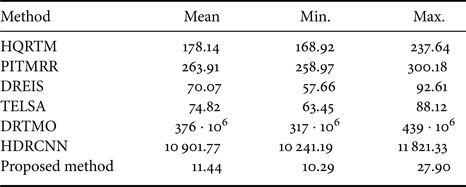
The mean, min, and max computation-times for processing each image from the test dataset were computed. Table 4 shows the results of this analysis. We found, as might be expected, that the mean computation-time of the proposed method ($11.44\,{\rm ms}\pm 2.23$ ) is far less than other methods. It also can be noticed that the methods based on Convolutional Neural Networks, DRTMO, and HDRCNN show the highest computation-times.
Table 4. Computation-time for processing one frame ($1920\times 1080$ ) in milliseconds (ms).
VI. CONCLUSIONS
In this paper, we have presented a fully-automatic inverse tone mapping operator and experimental results that show its effectiveness for rendering LDR content in modern HDR LED displays. We employed two full-reference objective metrics to compare our method against recent approaches. The proposed method was found to provide higher image quality scores in a number of test HDR-LDR datasets while achieving the lowest processing time. It can also be observed that with a maximum computation time of 27.90 ms, the proposed method can be considered as the most promising approach for real-time inverse tone mapping of HD ($1920\times1080$ ) video sequences at 24fps. Note that the maximum computing-time to process one frame of an HD video in real-time at 24 fps is 41.66 ms.
The novelty of our paper is to exploit the freedom that the proposed tone mapper function in mapping a human visual experiment to the parameters of the curve can offer. In this experiment, users tried to mimic the artistic intention of the grader. We found that the proposed inverse tone mapping method is able to generate believable scenes at different global brightness impressions, which we call different artistic intentions. Our research trains the parameters to follow the artistic intentions of a human grader.
The proposed method sets all parameters of its mid-level mapping function automatically, by modeling human perception using first-order image statistics. Moreover, the mapping function can be used in any type of HDR display, i.e. different levels of peak brightness. Because professionally-graded HDR images were used as a reference for this mapping procedure, the proposed method preserves the artistic intentions inherent to the HDR grading. This is reflected in better Q-scores obtained in the HDR-VDP-2.2 metric.
Despite the proposed method was developed to expand LDR static images, it can be used to expand an LDR video sequence frame by frame. The proposed algorithm has advantages when it comes to video: it is simpler, therefore allowing real-time processing and allowing better integration with integrated hardware. Also, it is less complex, leaving less room for errors. However, in order to extend our method to handling video sequences, a method to ensure temporal coherence of the middle-gray output value ($m_o$ ) between frames needs to be considered. This will prevent the inverse tone-mapped HDR video from flickering.
We also confirmed the findings made by Akyüz et al. [Reference Akyüz, Fleming, Riecke, Reinhard and Bülthoff31], which stated that, from a perceptual point of view, a sophisticated algorithm for inverse tone mapping is not necessary to yield a compelling HDR experience. In our case, our results produced on average a similar mean-opinion scores (Q-score) than more complex methods.
An important aspect of the proposed method, and in contrast to neural network approaches, is that the proposed methods' mapping procedure provides insight about the type of enhancement as expected by the observer of an HDR image while avoiding the need of an extensive training set. Although our experimental results are very promising, we acknowledge that exhaustive tests on the effect of mid-level mapping parameters should be carried out.
Despite the fact that a more exhaustive subjective evaluation is very relevant, the objective measures used in this paper can be seen as complementary and less subject to debate. Therefore, of interest to the community. While this objective evaluation is useful, in the future, it would be interesting to do an additional exhaustive subjective evaluation of the performance of the proposed method including other evaluation criteria.
Some of the drawbacks of the proposed method are mainly related to the contrast stretching by using a global expansion operator, such as false-contouring and noise-artifacts boosting. The stretched contrast results in an increase of visibility of compression artifacts and the appearance of false contours. The former issue was more related to artifacts in the LDR input image [Reference Reinhard, Kunkel, Marion, Brouillat, Cozot and Bouatouch48]. This is unavoidable and the best course of action is to combine it with a real-time denouncing algorithm prior to the proposed algorithm. The second drawback can be mitigated by using a method previously proposed by ours which helps to remove false contours in HDR images [Reference Luzardo, Aelterman, Luong, Philips and Ochoa49]. Another shortcoming we found in our method is related to the colorimetry. We used a fixed value of 1.25 for the saturation compensation on the HDR output, however, we think that further research in this aspect is needed. In future work, we are planning to work more in terms of pixel-wise saturation compensation. We found that better results can be obtained by locally varying the saturation enhancement parameter for every pixel. In this way, not every pixel will be boosted in color saturation the same way, resulting in HDR scenes that are a mix of objects with a muted color saturation and very colorful objects.
SUPPLEMENTARY MATERIAL
Supplementary material is available at http://telin.ugent.be/~gluzardo/midlevel-itmo
ACKNOWLEDGMENTS
The work of G. Luzardo was supported by Secretaría de Educación Superior, Ciencia, Tecnología e Innovación (SENESCYT), and Escuela Superior Politécnica del Litoral (ESPOL) under Ph.D. studies 2016. Jan Aelterman is currently supported by Ghent University postdoctoral fellowship (BOF15/PDO/003).
FINANCIAL SUPPORT
This work was supported by imec as part of the imec.ICON HD2R project.
Gonzalo Luzardo received his Master in Computer Science and Information Technology with specialization in Multimedia Systems and Intelligent Computing from Polytechnic University of Madrid in 2019. He is a tenured professor at ESPOL Polytechnic University (Ecuador) from 2010. Currently, he is following his PhD at Gent University and working as a doctoral researcher at the Image Processing and Interpretation (IPI) group, an imec research group at Ghent University. His research focus on real-time video processing, especially in HDR domain.
Jan Aelterman received his PhD in Engineering from Ghent University in 2014. Currently, he is working as a post-doctoral researcher at the Image Processing and Interpretation (IPI) group, an imec research group at Ghent University. His research deals with image and video restoration, reconstruction and estimation problems in application fields, such as (HDR) consumer video, MRI, CT, (electron)microscopy, photography and multi-view processing.
Hiep Luong received his PhD degree in Computer Science Engineering from Ghent University in 2009. He has been working as a postdoctoral researcher and project manager at Image Processing and Interpretation (IPI), an imec research group at Ghent University. Currently, he is assistant professor at IPI and leads the UAV Research Centre of UGent. His research and expertise focus on image and real- time video processing for various fields, such as HDR imaging, (bio)medical imaging, depth and multi-view processing, and multi-sensor fusion for UAV and AR applications.
Sven Rousseaux is part of the Research and Innovation Department in the Flemish Radio and Television Broadcasting Organization (VRT), Belgium. He has worked on medium-term research projects with Flemish as well as international partners. His expertise focus on subjects related to media production and media management.
Daniel Ochoa received his PhD degree in Computer Science Engineering from Ghent University in 2012. He has been working as researcher in the center for Computer Vison and Robotics (CVR) at ESPOL University. Currently, he is professor at ESPOL and leads CVR. His expertise and research focus is Hyperspectal Image acquisition, fusion and processing in biotechnological applications and embedded systems.
Wilfried Philips was born in Aalst, Belgium on October 19, 1966. In 1989, he received the Diploma degree in Electrical Engineering from the University of Gent, Belgium. Since October 1989 he has been working at the Department of Electronics and Information Systems of Ghent University, as a research assistant for the Flemish Fund for Scientific Research (FWO). In 1993 he obtained the Ph.D. degree in electrical engineering from Ghent university, Belgium. His main research interests are image and video restoration, image analysis, and lossless and lossy data compression of images and video and processing of multimedia data.


 Open access