


1. Introduction
A proper understanding of the microswimmer's biological functionality, i.e. predation (Magar, Goto & Pedley Reference Magar, Goto and Pedley2003; Magar & Pedley Reference Magar and Pedley2005; Peng & Dabiri Reference Peng and Dabiri2009; Soto & Golestanian Reference Soto and Golestanian2014; Jan & Löwen Reference Jan Schwarzendahl and Löwen2021), transport (Solovev et al. Reference Solovev, Sanchez, Pumera, Mei and Schmidt2010; Pushkin, Shum & Yeomans Reference Pushkin, Shum and Yeomans2013; Jin et al. Reference Jin, Chen, Maass and Mathijssen2021) and pick-up (Burdick et al. Reference Burdick, Laocharoensuk, Wheat, Posner and Wang2008; Gao et al. Reference Gao2011), plays a significant role in designing efficient swimming devices relevant for drug delivery, gene therapy and bionic applications. Recently, research on microswimming has been broadened to the inertial flow regime because some aquatic microswimmers can swim at a finite Reynolds number in the range of O(1)–(100) (Childress Reference Childress1981; Beckett Reference Beckett1986; Ishikawa & Hota 2006; Kiørboe, Jiang & Colin Reference Kiørboe, Jiang and Colin2010; Wickramarathna, Noss & Lorke Reference Wickramarathna, Noss and Lorke2014).
Proposed by Lighthill (Reference Lighthill1952) and extended by Blake (Reference Blake1971), the spherical squirmer model has been widely employed to mimic the self-propulsion of a swimmer with a dense array of cilia on its surface, such as Opalina and Volvox (Pedley, Brumley & Goldstein Reference Pedley, Brumley and Goldstein2016). This model has been successfully used in simulating the self-propelled organisms’ nutrient uptake (Magar et al. Reference Magar, Goto and Pedley2003; Magar & Pedley Reference Magar and Pedley2005), their hydrodynamic interactions with a wall (Ishimoto & Gaffney Reference Ishimoto and Gaffney2013; Ouyang, Lin & Ku Reference Ouyang, Lin and Ku2018a), the two-body hydrodynamic interactions (Ishikawa, Simmonds & Pedley Reference Ishikawa, Simmonds and Pedley2006; Götze & Gompper Reference Götze and Gompper2010; Navarro & Pagonabarraga Reference Navarro and Pagonabarraga2010; Ouyang, Lin & Ku Reference Ouyang, Lin and Ku2019) and their collective swimming (Ishikawa, Locsei & Pedley Reference Ishikawa, Locsei and Pedley2008; Ishikawa & Pedley Reference Ishikawa and Pedley2008; Zöttl & Stark Reference Zöttl and Stark2014). The ‘inertial squirmer’ at a finite Re has been analytically and numerically studied recently (Wang & Ardekani Reference Wang and Ardekani2012; Khair & Chisholm Reference Khair and Chisholm2014; Chisholm et al. Reference Chisholm, Legendre, Lauga and Khair2016; Li, Ostace & Ardekani Reference Li, Ostace and Ardekani2016; Ouyang, Lin & Ku Reference Ouyang, Lin and Ku2018b; Lin & Gao Reference Lin and Gao2019; More & Ardekani Reference More and Ardekani2020). These studies indicated that the fluid inertia had a significant impact on their swimming, both enhancing or hindering the speed of the swimmer (depending on the self-propelled modes), destabilizing the pusher (propelled from the rear), changing the contact time with a wall and weakening the collective dynamics.
Microorganisms in nature usually have an irregular non-spherical shape (Schaller et al. Reference Schaller, Weber, Semmrich, Frey and Bausch2010; Sanchez et al. Reference Sanchez, Chen, DeCamp, Heymann and Dogic2012; Wensink et al. Reference Wensink, Dunkel, Heidenreich, Drescher, Goldstein, Löwen and Yeomans2012), and the design of microswimming devices needs to incorporate non-spherical structures. Hence, the hydrodynamics of a squirmer dumbbell assembled by two or more squirmers has recently attracted attention. These assemblies are crucial for constructing more complex shapes, such as autonomous micro-robots (Ishikawa Reference Ishikawa2019), and new functional soft materials (Cates & MacKintosh Reference Cates and MacKintosh2011; Winkler & Gompper Reference Winkler and Gompper2020). A stability analysis revealed that the squirmer dumbbell could not achieve a stable forward swimming in the far-field without external torque, and fore-and-aft swimming is stable when the aft squirmer is a strong pusher (Ishikawa Reference Ishikawa2019). Clopés, Gompper & Winkler (Reference Clopés, Gompper and Winkler2020) investigated the swimming behaviour of a squirmer dumbbell and found that a pair of strong pullers (propelled from the front) was less efficient by an order of magnitude smaller in swimming efficiency than a pair of pushers. Zantop & Stark (Reference Zantop and Stark2020) found that a squirmer rod with a noticeable elongation could induce a flow field comprising four hydrodynamic moments: force dipole, source dipole, force quadrupole and source octupole. Ouyang & Lin (Reference Ouyang and Lin2021) investigated a squirmer rod swimming in a Newtonian fluid, and found that the fluid inertia, the number of the squirmers, the swimming mode and the gap between two adjacent squirmers could significantly affect its swimming speed, power expenditure and hydrodynamic efficiency. Additionally, the larger power-law index n for a power-law fluid yields a faster squirmer rod at Re ≤ 0.5, but a faster puller rod at Re ≥ 1 (Ouyang & Phan-Thien Reference Ouyang and Phan-Thien2021). More recently, Ouyang et al. (Reference Ouyang, Lin, Yu, Lin and Phan-Thien2022) considered the inertial swimming of a squirmer dumbbell inside a tube and found that the constrained tube could counterintuitively hasten an inertial pusher dumbbell.
These above results are for the microswimmer alone, whereas its predation, transportation and other functional behaviours (e.g. targeted drug delivery or performing tissue biopsy) require the microswimmer to carry a specific load. Raz & Leshansky (Reference Raz and Leshansky2008) considered a microswimmer towing a spherical load through a viscous fluid and found that an optimal propeller-load size ratio depended on the propeller efficiency and their mutual proximity, and the hydrodynamic interaction between the load and the propeller could enhance the dragging efficiency. Gao et al. (Reference Gao2011) experimentally investigated the efficient cargo-towing capabilities of magnetically driven nanomotors. They elucidated the fundamental mechanism of cargo-towing by the flexible nanoswimmers and assessed to what extent they could be used to transport a relevant cargo in biological media. Felderhof (Reference Felderhof2014) considered a spherical cargo driven by the tail of little spheres via hydrodynamic and direct elastic interactions. Their result showed that the estimates of the swimming speed based on Stokes’ law and the resistive force theory did not take proper account of the hydrodynamic interactions and led to an incorrect dependence of the swimming speed on the radius of the cargo. Debnath et al. (Reference Debnath, Ghosh, Li, Marchesoni and Li2016) proposed a working model of the active dimer's diffusion to quantify the efficiency of Janus particles (particles with two distinct surface physical properties) as cargo towers. They concluded that an active dimer exhibits optimal towing capability only in the puller and pusher configurations. Gutman & Or (Reference Gutman and Or2016) numerically studied the swimming of an undulating magnetic microswimmer carrying a spherical cargo and established the optimal combinations of frequency, stiffness and tail-cargo size ratio for maximizing either its displacement, mean speed or energetic efficiency. Debnath et al. (Reference Debnath, Ghosh, Nori, Li, Marchesoni and Li2017) studied the dynamics of an elastic dimer consisting of an active swimmer bound to a passive cargo in a Couette flow. They concluded that, due to the long-range hydrodynamic interactions, the dimer's diffusive properties depend on three parameters: the size of its constituents, its self-propulsion speed and the shear flow. Debnath & Ghosh (Reference Debnath and Ghosh2018) investigated the escape kinetics of a Janus particle (a self-propelled particle) carrying a cargo and found that hydrodynamic interactions could significantly enhance the escape rate of the Janus-cargo dimer. Daddi-Moussa-Ider, Lisicki & Mathijssen (Reference Daddi-Moussa-Ider, Lisicki and Mathijssen2020) explored the cargo transport by a three-body microswimmer in an external shear flow close to a planar boundary using fully resolved simulations. They found that cargo pullers were the fastest at most flow strengths, but pushers featured a non-trivial optimum that could be tuned by their geometry. Even though several aspects of the swimmer carrying a cargo are considered, these above efforts have been made in the limit of Stokes flow regime (the problem is linear at Re = 0). As mentioned above, fluid inertia can significantly affect the hydrodynamic behaviour of the swimmers with different self-propelled modes at a finite Re, and the inertial swimming problem requires the Navier–Stokes (N–S) equations to be solved in full. Accordingly, we still know little about how the fluid inertia affects the hydrodynamic interaction between the cargo and the propeller, and consequently, their swimming behaviour.
This paper employs a direct-forcing fictitious domain method (DF-FDM) to investigate a spherical squirmer dragging a rigid cargo in an infinite Newtonian fluid. The main emphasis of this study is to elucidate how the fluid inertia, the cargo shapes, and the relative position between the propeller and the cargo affect the assembly's hydrodynamics. We also expect to find potentially the most efficient cargo-carrying model. The remainder of this paper is organized as follows. Section 2 outlines the DF-FDM and the dynamics of the squirmer carrying a cargo in sufficient details. Subsequently, we validate the mesh and domain independence in § 3. In § 4, the results, including the assemblies’ swimming speeds, their energy expenditure, hydrodynamic efficiency, swimming stability and the drag force, are presented and discussed. Finally, some concluding remarks are given in § 5.
2. Physical description and numerical method
This section outlines the governing equations and the numerical method employed to simulate the motion of a propeller carrying a cargo through a Newtonian fluid. The incompressible Navier–Stokes (N–S) equations governing the fluid flow in the calculation domain  $\varOmega$:
 \begin{gather}{\rho _f}\frac{{\textrm{D}\boldsymbol{u}}}{{\textrm{D}t}} = \boldsymbol{\nabla }\boldsymbol{\cdot }\boldsymbol{\sigma },\quad \textrm{in}\ \varOmega ,\end{gather}
 \begin{gather}\boldsymbol{\nabla }\boldsymbol{\cdot }\boldsymbol{u} = 0,\quad \textrm{in}\ \varOmega ,\end{gather}
where  $\textrm{D}/\textrm{D}t = \partial \boldsymbol{u}/\partial t + \boldsymbol{u}\boldsymbol{\cdot }\boldsymbol{\nabla }\boldsymbol{u}$ is the material derivative, and ρf, u and σ are the fluid density, the fluid velocity and the fluid stress, respectively. Assuming that the spherical propeller and the cargo are rigid and linked by a phantom rigid rod (see figure 1), the whole body is governed by Newton's equations,
 \begin{gather}M\frac{{\textrm{d}\boldsymbol{U}}}{{\textrm{d}t}} = {\boldsymbol{F}^H} + \left( {1 - \frac{1}{{{\rho_r}}}} \right)M\boldsymbol{g},\end{gather}
 \begin{gather}\frac{{\textrm{d(}\boldsymbol{J}\boldsymbol{\cdot }{\boldsymbol{\omega }_s})}}{{\textrm{d}t}} = {\boldsymbol{T}^H},\end{gather}
where M, J, U and ωs are respectively the body's mass, its moment of inertia tensor, its translational velocity and its angular velocity; g is the gravitational acceleration; and ρr is the solid–fluid density ratio. Here, FH and TH are the hydrodynamic force and torque on the body, respectively, which are defined by
 \begin{gather}{\boldsymbol{F}^H} = \int_{\partial S} {\boldsymbol{n}\boldsymbol{\cdot }\boldsymbol{\sigma }\,\textrm{d}S} ,\end{gather}
 \begin{gather}{\boldsymbol{T}^H} = \int_{\partial S} {\boldsymbol{r} \times (\boldsymbol{n}\boldsymbol{\cdot }\boldsymbol{\sigma })\,\textrm{d}S} ,\end{gather}
where n is the unit outward normal on the surface S, and r is the position vector concerning the assembly's centre O (see figure 1). An interface-resolved direct-forcing (DF) fictitious domain method (FDM) (Yu & Shao Reference Yu and Shao2007), which fills the interior of the body with the fluid, and a pseudo body force is introduced over the body inner-domain to enforce the fictitious fluid to satisfy the rigid-body motion constraint, is adopted here to deal with hydrodynamic interactions between the body and the fluid. This scheme introduces a body-force λ in the solid body domain S 0(t) (as a Lagrange multiplier) and it reads
 \begin{equation}{\rho _f}\frac{{\textrm{D}\boldsymbol{u}}}{{\textrm{D}t}} = \boldsymbol{\nabla }\boldsymbol{\cdot }\boldsymbol{\sigma } + \boldsymbol{\lambda },\quad \textrm{in}\ {S_0}(t).\end{equation}
In the spherical squirmer model, a progressive waving envelope is introduced to mimic both radial and angular oscillations on the boundary of a microswimmer with arrays of cilia like Volvox (Pedley et al. Reference Pedley, Brumley and Goldstein2016). In the framework of FDM, the motion of the fluid-filled fictitious domain (domain occupied by the squirmer and the cargo) is hence governed by
 \begin{equation}\boldsymbol{u} = \boldsymbol{U} + {\boldsymbol{\omega }_s} \times \boldsymbol{r} + {\boldsymbol{u}_s},\end{equation}
where us is performed with the following divergence-free velocity field (in the frame of reference moving with the body) inside the squirmer (Li et al. Reference Li, Ostace and Ardekani2016; Lin & Gao Reference Lin and Gao2019; More & Ardekani Reference More and Ardekani2020):
 \begin{align}{\boldsymbol{u}_s} &= \left[ {{{\left( {\frac{{{r_s}}}{a}} \right)}^m} - {{\left( {\frac{{{r_s}}}{a}} \right)}^{m + 1}}} \right]\left( {u_\theta^s\cot \theta + \frac{{\textrm{d}u_\theta^s}}{{\textrm{d}\theta }}} \right){\boldsymbol{e}_r}\nonumber\\ &\quad + \left[ {(m + 3){{\left( {\frac{{{r_s}}}{a}} \right)}^{m + 1}} - (m + 2){{\left( {\frac{{{r_s}}}{a}} \right)}^m}} \right]u_\theta ^s{\boldsymbol{e}_\theta },\end{align}
where a is the radius of the squirmer, rs is the distance from the squirmer's centre, er and eθ are respectively the unit vectors along the radial and polar directions, and m is an arbitrary positive integer;  $u_\theta ^s$ is expressed as
 \begin{equation}u_\theta ^s(\theta ) = {B_1}\sin \theta + {B_2}\sin \theta \cos \theta ,\end{equation}
where θ is the angle concerning the swimming direction, and B 1 and B 2 are the swimming parameters. The mode of the squirmer can be defined as a puller (β > 0, e.g. Chlamydomonas), pusher (β < 0, e.g. Escherichia coli) and neutral squirmer (β = 0), based on the values of β = B 2/B 1 (B 1 > 0) (Ishikawa & Pedley Reference Ishikawa and Pedley2008). In the Stokes flow regime, the velocity of a squirmer in an infinite domain is U 0 = 2B 1/3 (Lighthill Reference Lighthill1952) and we adopt it as the velocity scale in this study.
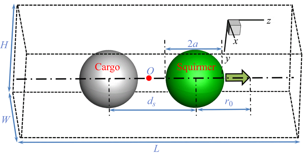
Figure 1. Schematic of a squirmer carrying a cargo in an infinite flow (the green and grey spheres represent respectively the squirmer and the cargo, and the blue arrow indicates the swimming direction).
Integrating (2.7) and r × (2.7) over the interior of the squirmer and cargo, and substituting it into (2.5) and (2.6) yields
 \begin{gather}{\boldsymbol{F}^H} = - \int_{{S_0}} {\boldsymbol{\lambda }\,\textrm{d}\boldsymbol{x}} + \frac{M}{{{\rho _r}}}\frac{{\textrm{d}\boldsymbol{U}}}{{\textrm{d}t}} + \int_{{S_0}} {{\rho _f}\frac{{\textrm{d}{{\boldsymbol{u}}_s}}}{{\textrm{d}t}}\,} \textrm{d}\boldsymbol{x},\end{gather}
 \begin{gather}{\boldsymbol{T}^H} = - \int_{{S_0}} {\boldsymbol{r} \times \boldsymbol{\lambda }\,\textrm{d}\boldsymbol{x}} + \frac{1}{{{\rho _r}}}\frac{{\textrm{d}(\boldsymbol{J}\boldsymbol{\cdot }{\boldsymbol{\omega }_s})}}{{\textrm{d}t}} + \int_{{S_0}} {{\rho _f}\left( {\boldsymbol{r} \times \frac{{\textrm{d}{\boldsymbol{u}_s}}}{{\textrm{d}t}}} \right)\textrm{d}\boldsymbol{x}} .\end{gather}
Substituting (2.11) into (2.3) and (2.12) into (2.4), we can hence solve the motion problem of the whole body. For the details of the squirmer dynamics employing the DF-FDM, one can refer to the work of Lin & Gao (Reference Lin and Gao2019).
3. Validation of mesh and domain independence
The DF-FDM simulation of squirmer dynamics has been shown to be accurate when compared with the theoretical solution at Re = 0 (Lin & Gao Reference Lin and Gao2019) and other numerical results at a finite Re (Ouyang et al. Reference Ouyang, Lin, Yu, Lin and Phan-Thien2022). Note that the swimming Reynolds number in this study is defined as Re = ρfaU 0/μ, and the velocities and the time are normalized by the velocity scale U 0 and time scale a/U 0, respectively. As shown in figure 1, we define four typical models based on the arrangement of the squirmer and the spherical cargo, namely, the pusher-cargo (pusher behind the cargo), puller-cargo (puller behind the cargo), cargo-pusher (pusher in front of the cargo) and cargo-puller (puller in front of the cargo). The squirmer and the cargo are assumed neutrally buoyant with identical volume. In this section, we perform the validations of the mesh size and the flow field independence with a possible extreme case (the maximum swimming speed confirmed in the next section, see figure 4), namely, the pusher-cargo (β = −3) model at Re = 100 (ds = 2a). The periodic boundary conditions are employed at all the boundaries to simulate the infinite flow field. The moving mesh technology, shifting the flow field and the body position one mesh distance once the body moves a horizontal position that is greater than the centre of the domain in the horizontal direction (z-axis), is employed to keep the assembly nearly at the centre of the calculated domain to save the computational resources. We initialize the assembly at the centre of the fluid field with its orientation directing along the z-axis, and its velocity reaches a steady state after the initial transient dynamics. Note that the assembly's translation and rotation in the x- and y-axes are restricted for better comparing the speeds (the unstable swimming may occur at the finite Re, see § 4.4) if not otherwise specified. This is because the axisymmetric vorticity around the squirmer may break at a finite critical Re (Chisholm et al. Reference Chisholm, Legendre, Lauga and Khair2016; Ouyang et al. Reference Ouyang, Lin and Ku2018b; Ouyang & Lin Reference Ouyang and Lin2021). Hence, the swimming speed U here denotes the velocity component of the assembly in the z-axis. Lin & Gao (Reference Lin and Gao2019) report that a mesh size with 32Δx across the diameter of an individual squirmer and a time step Δt less than 0.002 have been shown to be convergent. Here, we simulate the aforementioned case with three mesh sizes, namely, 24, 32 and 48Δx across the diameter of the squirmer or the cargo. We employ the height and width with H × W = 18a × 18a which have been shown to be convergent (More & Ardekani Reference More and Ardekani2020) to simulate the infinite fluid field in the x- and y-directions. We employ three typical lengths (L = 24, 36 and 48a in the z-direction) and compare the results.
Figures 2 and 3 present the steady speeds of the pusher-cargo model with different mesh sizes and domains. The convergent result can be obtained by using the mesh size with 32Δx across the diameter of the squirmer or the cargo and the computational domain with H × W × L = 18a × 18a × 36a. Hence, we employ these calculation parameters in the following simulations if not otherwise specified.

Figure 2. Swimming speed evolution for the pusher-cargo model with different mesh sizes at Re = 100. The velocity is normalized with the steady speed of the squirmer in Stokes flow, i.e. U 0 = 2B 1/3, and the time scale a/U 0 normalizes the time.

Figure 3. Swimming speed evolution for the pusher-cargo model with different domains at Re = 100.
4. Results and discussion
A squirmer (β = ±3) carrying a cargo in an infinite fluid field is conducted in this section with the swimming Reynolds number in the range of 5 ≤ Re ≤ 100. We first consider the effect of the relative position (the distance ds and the four different assembled models) between the squirmer and the spherical cargo on the assembly's locomotion. Subsequently, we investigate the effects of the cargo's geometry (i.e. spherical, oblate and prolate cargoes) and orientation on the assembly's locomotion. We also obtain and discuss the energy expenditure of these assemblies and their carrying hydrodynamic efficiency. Finally, the swimming stability of these assemblies is presented and analysed.
4.1. Pusher-cargo model achieves a significantly faster swimming speed
Keeping the squirmer and the cargo in contact (ds = 2a), it is seen that the pusher-cargo model swims significantly faster than the remaining three models at a finite Re adopted in this study (see figure 4). The pusher-cargo model with β = −3 and ds = 2a, for example, can swim approximately 320 % (180 %) faster than the counterpart cargo-pusher model at Re = 25 (Re = 100). Note that these speeds are obtained by taking a time average once the transients die out. This pattern is similar to that of an individual squirmer's speed with a finite fluid inertia (Li et al. Reference Li, Ostace and Ardekani2016). The cargo-pusher model, nevertheless, has not shown the advantage of the ‘pushed-type’ propeller. To illustrate the possible mechanism for these results, we plot the velocity magnitude and vorticity contours, as shown in figures 5 and 6. This is because the vorticity generated around the individual squirmer's body significantly affects its swimming speed at a finite Re (Chisholm et al. Reference Chisholm, Legendre, Lauga and Khair2016; Li et al. Reference Li, Ostace and Ardekani2016; Ouyang et al. Reference Ouyang, Lin and Ku2018a; More & Ardekani Reference More and Ardekani2020). From these results, it can be concluded that, with increasing Re, a puller ‘pulls’ the vorticity (generated by the puller) to accumulate around the body with increase in the inertia of the body (hence hindering its speed, see figure 6(d), the vorticity around the green puller), whereas a pusher ‘pushes’ the vorticity (generated by the pusher) downstream hence speeding up (see figure 6(e), the vorticity around the green pusher). The pusher-cargo model's speed clearly shows a similar pattern to that of an individual pusher, because the front cargo has not affected the downstream of the vorticity (see figure 6e). Since the cargo behind the pusher hinders the convection downstream of the vorticity (see figure 5e), the cargo-pusher model's speed is suppressed. In contrast, it is seen that the cargo behind the puller contributes to the convection downstream of the vorticity at Re = 25 (see figure 5d). Hence, the cargo-puller model swims slightly faster than the puller-cargo model (see figure 4, Re = 25). The velocity of the flow in front of the cargo-puller model is observed to decay more rapidly than that for the cargo-pusher model at Re = 25, as shown in figures 5(a) and 5(b). This result proves that the cargo-puller model swims faster than the cargo-pusher model, where a more rapid decay of the velocity in front of the body leads to a faster swimmer (Zhu et al. Reference Zhu, Do-Quang, Lauga and Brandt2011).

Figure 4. Steady swimming speed for a squirmer carrying a cargo in an infinite fluid field at different Re. The speed denotes the velocity component in the z-axis and is normalized with the steady speed in Stokes flow, i.e. U 0 = 2B 1/3. Here, amin and amax respectively denote the cargo radii with 0.5a and 2a. The time is normalized with the time scale a/U 0.

Figure 5. Comparing the flow fields around the squirmer and the cargo with |β| = 3 at Re = 25: (a–c) velocity magnitude contours; (d–f) vorticity contours. The green sphere denotes the squirmer and the grey one denotes the cargo. (a,d) cargo-puller model; (b,c,e,f) cargo-pusher model. (a,b,d,e) ds = 2a; (c,f) ds = 3a. The velocity magnitude is normalized with 2B 1/3.

Figure 6. Comparing the flow fields around the squirmer and the cargo with |β| = 3 at Re = 25: (a–c) velocity magnitude contours; (d–f) vorticity contours. The green sphere denotes the squirmer and the grey one denotes the cargo. (a,d) Puller-cargo model; (b,c,e,f) pusher-cargo model. (a,b,d,e) ds = 2a; (c,f) ds = 3a. The velocity magnitude is normalized with 2B 1/3.
The distance between the propeller and the cargo can also affect the assembly's swimming speed, as shown in figure 4. The cargo-pusher model with a larger ds yields a faster speed. This is because a larger ds contributes to the convection downstream of the vorticity (see figures 5e and 5f), and the hydrodynamic interaction between the squirmer and the cargo with a narrow gap (ds = 2a) hinders the vorticity being pushed away. Hence, a thicker vorticity in front of the squirmer is observed with ds = 2a than ds = 3a and, accordingly (see figures 5b and 5c), a smaller velocity gradient, an indication of a slower velocity decay, in front of the assembly is seen with ds = 2a than ds = 3a). Meanwhile, the pusher-cargo model with a larger ds yields a slower speed. This is because the vorticity adheres to the body with ds = 3a (see figure 6f) more than ds = 2a (see figure 6e). It is seen that the puller-cargo model induces a significantly smaller velocity magnitude in front of the body than the pusher-cargo model (see figures 6a and 6b), corresponding to the apparent swimming speed difference between them (see figure 4). For the pusher-cargo model, it is also seen that a smaller cargo results in a faster speed as the smaller cargo size corresponds to a smaller frontal area and mass.
Figures 7(a) and 7(b) show an individual inertial squirmer swimming in an infinite fluid, in which a pusher (puller) is ‘pushed’ (‘pulled’) to swim faster (slower) by the flow field induced at an earlier time (denoted by the solid arrows) (Li et al. Reference Li, Ostace and Ardekani2016). This illustration can be broadened to the case of a squirmer carrying a cargo. It is seen that, with the pusher being arranged at the rear of the assembly, in the pusher-cargo model, the flow speeds up the body (see figure 7d, the solid arrows). By comparison, the cargo-pusher model is subject to the action of the flow in the opposite directions (the effect of the solid arrows of figure 7f is weaker in speeding up the assembly than that of figure 7d), because the pusher is arranged in the front of the assembly. Hence, the pusher-cargo model can swim faster than the cargo-pusher model (see figure 4). On a puller carrying a cargo, it is seen that the cargo-puller model swims faster than the puller-cargo model at Re ≤ 25 (see figure 4). This result could be explained by the fact that the cargo-puller model is subject to a weaker effect of the inertial flows in hindering its swimming than the puller-cargo model (comparing the solid arrows in figures 7c and 7e). By increasing Re, nevertheless, the speed of the puller-cargo gradually exceeds that of the cargo-puller. Recall the pattern of an individual puller's speed (β > 1) with Re – while the puller is ‘pulled’ to swim slower with Re at the first stage, and this trend fails beyond a critical Re (depends on β). Note that the trailing vortical wake bubble of a puller here with β > 1 resembles a Hill's spherical vortex (Chisholm et al. Reference Chisholm, Legendre, Lauga and Khair2016) and Fornberg (Reference Fornberg1988) indicated the presence of a Hill's vortex-like wake structure behind a sphere held fixed in a uniform flow, within which W/ρ (the maximum vorticity to the distance from the z-axis) is nearly constant once Re is sufficiently large. This leads to the convection downstream of the vorticity (More & Ardekani Reference More and Ardekani2020) and hence restores its speed. Accordingly, the cargo at the rear of the assembly (cargo-puller) may hinder the convection downstream of the vorticity. Hence, it has a larger carried vorticity than the cargo in the front of the assembly (puller-cargo). Consequently, the puller-cargo model may have less vorticity adhering to the body (hence, the puller-cargo model swims faster because the vorticity hinders the swimming speed) than the cargo-puller model when increasing Re (Re > 25).

Figure 7. Schematic to compare the swimming mechanisms between an individual inertial squirmer and a squirmer carrying a cargo (ds = 2a) in an infinite fluid field: (a) a puller; (b) a pusher; (c) a puller-cargo model; (d) a pusher-cargo model; (e) a cargo-puller model; (f) a cargo-pusher model. The dashed and solid squirmers and squirmers carrying a cargo are respectively represented at the previous and current instants. The dashed boundary lines represent the periodic conditions. All the blue arrows indicate the flows induced at the previous instant, and the solid ones denote the flows affecting the squirmers and squirmers with a cargo at the current instant.
We would like to consider the contribution of the hydrodynamic forces on the surface of the assemblies to illustrate the possible mechanism for why the speed of the puller-cargo configuration gradually exceeds the cargo-puller configuration as Re increases. For a steady swimming squirmer (assembly) in a Newtonian fluid, the net force on the body can be decomposed into pressure and viscous contributions, and in the swimming direction (z-axis), it has  ${F_z} = F_z^{pres} + F_z^{visc} = 0$. Note that the pressure force and the viscous force have the following forms:
 \begin{gather}F_z^{pres} ={-} \int_{\partial S} {p \cdot {n_z}\,\textrm{d}S} ,\end{gather}
 \begin{gather}F_z^{visc} = {\eta _s}\int_{\partial S} {\left[ {2{n_z}\frac{{\partial {u_z}}}{{\partial z}} + {n_x}\left( {\frac{{\partial {u_z}}}{{\partial x}} + \frac{{\partial {u_x}}}{{\partial z}}} \right) + {n_y}\left( {\frac{{\partial {u_z}}}{{\partial y}} + \frac{{\partial {u_y}}}{{\partial z}}} \right)} \right]\textrm{d}S} ,\end{gather}
where  ${\eta _s}$ denotes the viscosity of the fluid and n is the unit normal outward from the surface S of the assembly (nz denotes the component of n in the z-axis). The force contribution of the assemblies is shown in table 1, in which the forces are normalized with $0.5\rho U_0^2{\rm \pi} {a^2}$, and the gap ds = 2a for the assemblies is considered here. It is seen that the total forces Fz slightly deviate from zero. We would like to explain that it is challenging to accurately calculate the integrals on the boundary of assemblies numerically ((4.1) and (4.2)), because there is an extraordinary gradient of the physical quantity near the boundary, and a higher resolution of the mesh requires a significantly increased calculating cost (our code is based on the uniform mesh for the whole calculating domain). We expect that our results can broadly reflect the contribution of these forces. It is seen that the viscous force has a positive contribution in driving the assemblies, in contrast to the pressures. For the puller carrying a cargo (the identical propeller), we find a larger viscous force corresponds to a slower assembly. This may be because a greater viscous force leads to more dissipated energy in the flow field (for a specified propeller, it may swim slower as more energy is dissipated).
Table 1. Force contribution on the assemblies in the swimming direction (z-axis).

4.2. Oblate spheroid-shaped cargo benefits in hastening the pusher-type assemblies
This section considers the cargo geometry on the assembly's swimming. We will compare the swimming behaviour of three different assemblies, namely, the spherical, oblate and prolate cargoes carried by a pusher, expecting to obtain the most efficient assembly. Note that these cargoes are set to be an identical volume 3/4 ${\rm \pi}$a 3, and we hence adopt the radii of rotational axis ap = 1.2a and 0.8a, the aspect ratios (ar = cp/ap, cp denotes the length of the symmetric axis) ar = 0.5787 and 1.9531 respectively for the oblate and prolate cargoes. In the simulations, the distance between the squirmer's and cargo's mass centre is set to ds = 3a. The main finding in this section is that, as shown in figure 8, both the pusher-cargo and cargo-pusher assemblies with an oblate cargo swim faster than the corresponding assemblies with a spherical or prolate cargo. At Re = 25 (100), for example, the cargo-pusher assembly with an oblate cargo can swim approximately 12 % (24 %) faster than that with a spherical cargo. The corresponding increased ratios of the speed for the pusher-cargo assemblies are respectively 31 % at Re = 25 and 28 % at Re = 100.

Figure 8. Steady swimming speed for a pusher carrying a cargo with different geometries in an infinite fluid field at different Re. Model, model 1 and model 2 denote the spherical, prolate and oblate cargo, respectively.
Figures 9(a) and 9(b) show the flow fields around the cargo-pusher assemblies with β = −3 at Re = 25. It is seen that the velocity magnitude around the oblate cargo is generally greater than that around the prolate one, indicating that the former benefits in the swimming of the front pusher (the gap between the oblate cargo and the pusher is larger than that of the case with the prolate cargo). Figures 9(c) and 9(d) show the vorticity contours around these cargo-pusher assemblies. Since the geometries of these assemblies are significantly different, it is not easy to illustrate the mechanisms for the different swimming speeds by analysing the convection downstream of the vorticity. It seems that the cargo-pusher assembly with an oblate cargo generates more vorticity than a prolate one, but a larger gap (oblate cargo case) helps in the flowing at the rear of the pusher. Figure 10 shows the flow fields around the pusher-cargo assemblies with β = −3 at Re = 25. Similar to the cargo-pusher assemblies, the oblate cargo induces a greater velocity magnitude and vorticity than the prolate one. Note that Figures 9(e,f) and 10(e,f) show the top views in the z-axis direction.

Figure 9. Comparing the flow fields around the cargo-pusher model with β = −3 at Re = 25: (a,b) velocity magnitude contours; (c,d) vorticity contours; (e,f) top views in the z-axis direction for panels (a,b), respectively. (a,c) Cargo-pusher model 2; (b,d) cargo-pusher model 1. The green sphere denotes the squirmer and the grey one denotes the cargo. (a,c) Oblate cargo; (b,d) prolate cargo. The velocity magnitude is normalized with 2B 1/3.

Figure 10. Comparing the flow fields around the pusher-cargo model with β = −3 at Re = 25: (a,b) velocity magnitude contours; (c,d) vorticity contours; (e,f) top views in the z-axis direction for panels (a,b), respectively. (a,c) Pusher-cargo model 2; (b,d) pusher-cargo model 1. The green sphere denotes the squirmer and the grey one denotes the cargo. (a,c) Oblate cargo; (b,d) prolate cargo. The velocity magnitude is normalized with 2B 1/3.
The velocity decay of the flows in front of the assemblies may explain the cause of the different speeds. In an infinite fluid field with Re = 0, the velocity in front of an individual squirmer decays as |u| ≈ O(r −2). This is because the two terms on the right-hand side of (2.10) represent a potential dipole which decays as |u| ≈ O(r −3) and a stresslet which decays as |u| ≈ O(r −2), respectively. In contrast, numerical simulations show that this velocity decays as |u| ≈ O(r −3) for a squirmer at a finite Re (Li et al. Reference Li, Ostace and Ardekani2016; More & Ardekani Reference More and Ardekani2020). Figure 11 shows the velocity decay with r 0 from the centre of the squirmer or the cargo, and the velocity |u| and the distance r 0 are respectively normalized with the characteristic swimming speed 2B 1/3 and the radius a of a squirmer. It is seen that the velocity of the cargo-pusher assembly with an oblate cargo (|u| ≈ O(r −5)) decays faster than that with a prolate cargo (|u| ≈ O(r −4)) at Re = 25. This pattern is different from that of an individual squirmer because the carried cargoes change the structure of the flow field for these assemblies. However, this result indicates that a more rapid decay leads to larger efficiency (Zhu et al. Reference Zhu, Do-Quang, Lauga and Brandt2011; Ouyang et al. Reference Ouyang, Lin, Yu, Lin and Phan-Thien2022). The pusher-cargo assemblies with different-shaped cargoes maintain the same decay as |u| ≈ O(r −4) at the first stage (r/a < 2.5); by further increasing r/a, the velocity decay for the pusher-cargo model 2 is faster than that for the pusher-cargo model 1. It seems difficult to conclude by comparing our results with those for an individual squirmer because the existence of these cargoes completely changes the front swimming characteristics induced by an individual squirmer.

Figure 11. Effects of the different cargoes and the assemblies on the far-field flow structure at Re = 25. Here, r 0/a gives the location in front of the pusher or cargo in the direction of the z-axis (as shown in Figure 1, r 0/a = 1 is the location at the surface and in front of the pusher or cargo).
As the cargo may be acquired accidentally by a squirmer, the orientation of the cargo can affect the swimming speed of the assembly. Figure 12 presents the steady speeds for the pusher-cargo and cargo-pusher assemblies (β = −3) with their cargoes maintaining different orientations (0 ≤ α ≤ 90°; the cases in figures 9 and 10 indicate α = 0). Note that the breaking of the axisymmetric assembly may lead to a lateral displacement; we hence restrict the translations in the y- and x-axes here. The pusher-cargo assembly with a prolate cargo maintains a slower speed than that with the oblate cargo when increasing α, and the former (latter) decreases (increases) monotonically by 20 % (18 %) at Re = 25. This pattern (the variation with α) is also applicable to the cargo-pusher assemblies. This is because a larger α contributes to the convection downstream of the vorticity induced by a pusher more efficiently for the oblate cargo, but more difficult for the prolate one. We find the increase (decrease) rate usually occurs at 30° ≤ α ≤ 60°, indicating a violent rate of change for the assembly's carrying ability of the vorticity here. In addition, figure 12 also presents the frontal area SA for these different cargoes with α (the incoming is in the z-axis direction). It is seen that a larger SA corresponds to a smaller swimming speed for the assembly, in agreement with the hydrodynamic mechanism of navigation.

Figure 12. Steady swimming speeds for the pusher-cargo and cargo-pusher models with different cargo shapes and orientations at Re = 25 (left tick label); frontal area for the cargos with different orientations (right tick label).
4.3. Energy expenditure and carrying hydrodynamic efficiency
For a squirmer carrying a cargo in a Newtonian fluid, the rate of work P can be written as (More & Ardekani Reference More and Ardekani2020)
 \begin{equation}P ={-} \int_{\partial S} {(\boldsymbol{u}\boldsymbol{\cdot }\boldsymbol{\sigma })\boldsymbol{\cdot }\boldsymbol{n}\,\textrm{d}S} = \int_{\varOmega - {S_0}} {2\mu \boldsymbol{E}:\boldsymbol{E}\,\textrm{d}\varOmega } ,\end{equation}
where n is the unit normal outward from the surface S of the assembly; σ,  $\boldsymbol{E}$ and ${S_0}$ are respectively the stress tensor, the strain rate tensor and the solid body domain. In this paper, we define a carrying hydrodynamic efficiency η = P*/P, in which P* denotes the power necessary to move the spherical cargo ( ${P^\ast } = 0.5\rho {U^3}{\rm \pi} {a^2}{C_d}$ with the drag coefficient ${C_d} = 0.29238 \times {(1 + 9.06/{(2Re)^{0.5}})^2}$; Abraham 1970) at the assembly's swimming speed U. Figure 13 shows the energy expenditure for the steady swimming of a squirmer carrying a cargo in an infinite fluid. Note that P 0 denotes the normalized P with $4B_1^2\mu a/9$. It is seen in figure 13(a) that P for a squirmer carrying a cargo increases monotonically with Re, similar to the pattern of P for an individual squirmer swimming in an infinite fluid field (Chisholm et al. Reference Chisholm, Legendre, Lauga and Khair2016). This energy is generated by the second term on the right of (2.10) (self-propelling) and the hydrodynamic interaction between the squirmer and the cargo, and is dissipated by the viscous fluid. A greater ds results in expending less energy on the assembly. This may be because a greater ds weakens the hydrodynamic interaction between the squirmer and the cargo more than a smaller ds, leading to less viscous dissipation. The pusher-cargo (cargo-pusher) model expends more energy than the puller-cargo (cargo-puller) model. This result seems difficult to be explained as the contribution of the self-propelling and the hydrodynamic interaction with the cargo cannot be clarified. The effect of the cargo's geometry on P is shown in figure 13(b). The pusher-cargo (cargo-pusher) model with a spherical cargo expends the least energy, followed by that with a prolate one and then that with an oblate one. Figure 14 shows the carrying hydrodynamic efficiency η with Re. The pusher-cargo model is significantly more efficient than the other models, and a larger ds yields a smaller η for the pusher-cargo model, but a greater η for the cargo-pusher model (see figure 14a). This pattern is similar to that of the speed for these assemblies as in § 4.1, and the monotonic increase agrees with the result for an individual squirmer swimming in a bulk fluid (Chisholm et al. Reference Chisholm, Legendre, Lauga and Khair2016). Figure 14(b) reproduces the efficient pusher-cargo models carrying different shaped cargo. The prolate cargo yields the highest efficiency in the cargo-pusher models than the other cargos. This may be because the prolate cargo has the smallest frontal area (the minimum possible resistance) in the swimming direction (z-axis).

Figure 13. Energy expenditure for the steady swimming of a squirmer carrying a cargo in an infinite fluid with different Re: (a) squirmer carrying a spherical cargo; (b) squirmer carrying a cargo with different geometry.

Figure 14. Hydrodynamic efficiency for the steady swimming of a squirmer carrying a cargo in an infinite fluid with different Re: (a) squirmer carrying a spherical cargo; (b) squirmer carrying a cargo with different geometry.
4.4. Fluid inertia destabilizes swimming
Chisholm et al. (Reference Chisholm, Legendre, Lauga and Khair2016) report that fluid inertia induces unstable swimming for an individual puller because the body perturbed from the original trajectory is pushed to deviate from the trajectory due to the flow induced earlier (Li et al. Reference Li, Ostace and Ardekani2016; More & Ardekani Reference More and Ardekani2020). This critical Reynolds number is approximately Re ~ O(40) for the puller with β = 3. Note that we consider a motion off the original orbit as unstable (lateral displacement) and the aforementioned restriction in the lateral direction is removed in this section.
Figure 15 summarizes the stable and unstable motion of a squirmer carrying a cargo across Re. The main finding in this section is that the puller-cargo model is more stable than the cargo-puller model, in which the critical Re is approximately O(60) for the puller-spherical cargo model (ds = 2a) but approximately O(50) for the spherical cargo-puller model (ds = 2a). To illustrate the possible mechanism of the unstable swimming, we plot a schematic as shown in figure 16. The assembly initially swims along a straight line (see the centreline and the induced flows). A random perturbation results in a departure from the original orbit, and the induced flows by the assembly will determine its swimming stability. For an individual squirmer in a bulk fluid, an inertial puller (pusher) perturbed from its straight-line trajectory is pushed away (pulled towards) the original trajectory due to the flow induced earlier, making it unstable (stable) with increasing Re (Li et al. Reference Li, Ostace and Ardekani2016; More & Ardekani Reference More and Ardekani2020). This mechanism applies to the assemblies (see figure 15, the pusher-cargo and cargo-pusher models are stable with increasing Re, but the corresponding puller-type models become unstable with Re). The cargo-puller model off the original trajectory suffers the effect of the flows in pushing it departing from the centreline more than that for the puller-cargo model (see figures 16a and 16c, the sum of the solid blue arrows applied to the cargo-puller model is more significant than that to the puller-cargo model).

Figure 15. A polar phase diagram indicating the stable and unstable assemblies. Here, Ss, Se and So denote the spherical, prolate and oblate cargo, respectively; ds 1 = 2a, ds 2 = 3a.

Figure 16. Schematic to reveal and compare the swimming stability between the squirmer-cargo and cargo-squirmer in an infinite fluid field. The dashed and solid squirmers respectively denote them at the previous and current instants. The solid and dashed blue arrows respectively denote the flows induced at the previous and current instants. (a) Puller-cargo model; (b) pusher-cargo model; (c) cargo-puller model; (d) cargo-pusher model.
In addition, the assemblies with a larger ds (ds = 3a) tend to become unstable more easily, similar to the pattern of the stability for a puller dumbbell (two pullers assembled in tandem). This is because the body with a larger ds suffers the effect of the flows it induced in pushing away from the original orbit more significantly than that with a smaller ds (Ouyang & Lin Reference Ouyang and Lin2021; Ouyang et al. Reference Ouyang, Lin, Yu, Lin and Phan-Thien2022). This mechanism may also cause the stability of a squirmer carrying a cargo with different geometries – an assembly with an oblate cargo is more stable than that with prolate cargo, because the former (as the case with a larger ds) is more slender than the latter one.
To strengthen the possible mechanism of the unstable swimming for a squirmer carrying a cargo, we also consider the distribution of the pressure near an individual squirmer at Re = 25 for simplicity, as shown in figure 17. This is because the instability mechanism for a squirmer carrying a solid cargo is generally determined by the squirmer's self-propelling mode. We have mentioned above the flows affecting the squirmer which is deviated from the original orbit. Accordingly, when a puller is perturbed from its straight-line trajectory (see figure 17a, the solid circle), the net pressure around the body tends to push it away from the original trajectory (the net pressure directs towards the left side). In contrast, for the pusher perturbed from its straight-line trajectory (see figure 17b, the solid circle), the net pressure around the body tends to pull it returning to the original trajectory (the net pressure here directs towards the right side). Hence, the inertial pusher (puller) presents a stable (unstable) swimming pattern in an infinite fluid field. In other words, the puller is at the high-pressure area where the pressure on both sides decreases outward, and hence it is easy to be unstable when disturbed with a deviation; in contrast, the pusher is at the low-pressure area laterally, so it is relatively stable. Note that we display the pressure inside the squirmer for a better exhibition of the pressure around the body.

Figure 17. Pressure distribution around the squirmer in the infinite fluid field at Re = 25: (a) a puller with β = 3; (b) a pusher with β = −3. The dotted and the solid circulars respectively represent the squirmer at its original trajectory and the perturbed position. The arrows point in the direction of net pressure.
4.5. Carry force
From the perspective of manufacturing microswimming devices for cargo carrying, a greater force may result in a more difficult assembly to construct due to risk of breakage of the bond between swimmer and cargo. Hence, the drag coefficient Cs (the drag force normalized with  $0.5\rho U_0^2{\rm \pi} {a^2}$) when carrying the cargoes in an infinite fluid field at different Re is obtained, as shown in figure 18. It is seen that Cs decreases monotonically with Re, similar to the pattern of dragging a sphere (Re < 100). The drag coefficient of pusher-cargo model 2 is significantly larger than that of the other models, corresponding to a faster swimming speed of pusher-cargo model 2 (see figure 8). This hydrodynamic mechanism is also subtle to illustrate because the complex fluid fields around the assemblies are difficult to compare quantitatively here, and systematically considering the dynamics of a passive particle (squirmer) in the wake of a squirmer (sphere) is required in our future work.

Figure 18. Drag coefficient for a pusher carrying a cargo with different geometries in an infinite fluid field at different Re. Model, model 1 and model 2 denote the spherical, prolate and oblate cargo, respectively.
5. Conclusion
An interface-resolved simulation on the hydrodynamics of a spherical squirmer carrying a cargo in an infinite fluid field is conducted in this paper. A given tangential velocity (squirmer model) is employed at the surface of a spherical propeller for self-propelling, and a cargo is linked to the propeller by a phantom rigid rod to form the assembly. The effects of the fluid inertia, the cargo shapes, the assembled models and the relative distances (ds) between the squirmer and the cargo on the hydrodynamics of the assembly are studied. Therefore, the assemblies’ speed, swimming stability, energy expenditure and carrying hydrodynamic efficiency (η) are considered.
The results show that the pusher-cargo model swims significantly faster than the remaining three models at a finite Re. The cargo-pusher model, nevertheless, has not shown the advantage of the ‘pushed-type’ propeller. This is because the pusher-cargo model is similar to an individual pusher which ‘pushes’ the vorticity (generated by the pusher) downstream hence increasing its speed. The cargo-pusher model's speed, however, is suppressed as the cargo behind the pusher hinders the convection downstream of the vorticity.
It is also found that both the pusher-cargo and cargo-pusher assemblies with an oblate cargo swim faster than the corresponding assemblies with a spherical or prolate cargo. This may be because the velocity magnitude around the oblate cargo is generally greater than that around the prolate one (the former benefits in the swimming of the front pusher). Regarding the case that the cargo is acquired accidentally, the pusher-cargo assembly with a prolate cargo maintains a slower speed than that with an oblate cargo when increasing the included angle α, and the former (latter) decreases (increases) monotonically by 20 % (18 %) at Re = 25. This may be because a larger α contributes to the convection downstream of the vorticity induced by a pusher more efficiently for the oblate cargo, but less efficiently for the prolate one.
We find a greater ds results in expending less energy on the assembly. This may be because a greater ds weakens the hydrodynamic interaction between the squirmer and the cargo more than a smaller ds, leading to less viscous dissipation. The pusher-cargo (cargo-pusher) model with a spherical cargo expends the least energy, followed by that with a prolate one and then that with an oblate one. The pusher-cargo model is significantly more efficient than the other models, and a larger ds yields a smaller η for the pusher-cargo model, but a greater η for the cargo-pusher one.
Additionally, we find the puller-cargo model is more stable than the cargo-puller model, in which the critical Re is approximately O(60) for the puller-spherical cargo model (ds = 2a) but approximately O(50) for the spherical cargo-puller model (ds = 2a). This is because the cargo-puller model off the original trajectory suffers the effect of the flows in pushing it away from the centreline more than that for the puller-cargo model.
Funding
The authors would like to thank the Major Program of National Natural Science Foundation of China (Grant Nos. 12132015) and National Natural Science Foundation of China (Grant Nos. 12172327; 12072319).
Declaration of interests
The authors report no conflict of interest.
Data availability statement
The data that support the findings of this study are available from the corresponding author upon reasonable request.


