


Introduction
Several lines of evidence suggest that the mean energy requirements and metabolic rates of metazoans have generally increased through time (Bambach Reference Bambach1993; Payne and Finnegan Reference Payne and Finnegan2006; Finnegan et al. Reference Finnegan, McClain, Kosnik and Payne2011; Payne et al. Reference Payne, Heim, Knope, McClain and Payne2014; Smith et al. Reference Smith, Payne, Heim, Balk, Finnegan, Kowalewski, Lyons, McClain, McShea, Novack-Gottshall, Anich and Wang2016). A variety of potential intrinsic (e.g., physiological/behavioral/ecological) and extrinsic (environmental) drivers have been invoked to explain this long-term trend (Bambach Reference Bambach1993; Vermeij Reference Vermeij1995; Bush and Bambach Reference Bush and Bambach2011; Klompmaker et al. Reference Klompmaker, Kowalewski, Huntley and Finnegan2017), but no consensus view has yet emerged. This is due, in part, to the inherent limitations of studying fossil organisms: in most cases metabolic rates must be inferred from a combination of body-mass estimates, independent estimates of important environmental parameters, and physiological inferences from comparison with extant relatives (Finnegan et al. Reference Finnegan, McClain, Kosnik and Payne2011; Payne et al. Reference Payne, Heim, Knope, McClain and Payne2014; Heim et al. Reference Heim, Knope, Schaal, Wang and Payne2015; Strotz et al. Reference Strotz, Saupe, Kimmig and Lieberman2018). Such analyses are further complicated by the fact that, without additional data, it is impossible to separate the contributions of growth rate and longevity to body size in fossil organisms (Jones Reference Jones and McKinney1988).
Organisms that grow mineralized skeletons by marginal accretion (including many marine invertebrate groups such as corals, sponges, brachiopods, and mollusks) have the potential to provide more precise information about metabolic rates. These organisms commonly preserve their ontogenetic histories as seasonal variation in the physical properties and/or isotopic composition of accreted skeletal material (Jones and Quitmyer Reference Jones and Quitmyer1996) and can therefore provide a detailed record of individual growth rate through time and ultimate longevity.
Bivalve mollusks are diverse and abundant in the fossil record, and their skeletal growth is especially well-understood among taxa that grow by marginal accretion (Gosling Reference Gosling2015a). Consequently, they can serve as a useful model system for studying metabolic rate variation across space and time. However, before interpreting such rate variation in the fossil record, it is useful to first address three questions about extant bivalves:
1. Which environmental factors have the greatest influence on growth rates?
2. How much of an influence does evolutionary history (e.g., phylogenetic relatedness) have on growth rates?
3. How much of the total variation in bivalve growth rates can be explained by environmental variation and evolutionary history?
We address these questions by evaluating temperature, primary production, and evolutionary history as predictors of growth rate in bivalves. Salinity has also been found to interact with growth rate in bivalves, but the nature of this relationship is not straightforward, has been subject to very limited study, and may only be relevant at very low salinities (Seed and Suchanek Reference Seed, Suchanek and Gosling1992), so we do not consider it here. Temperature and food availability are well studied as predictors of growth rate within species, and positive relationships are generally recovered (e.g., Beukema and Cadee Reference Beukema and Cadee1991; Seed and Suchanek Reference Seed, Suchanek and Gosling1992; Savina and Pouvreau Reference Savina and Pouvreau2004; Bourlès et al. Reference Bourlès, Alunno-Bruscia, Pouvreau, Tollu, Leguay, Arnaud, Goulletquer and Kooijman2009; Chauvaud et al. Reference Chauvaud, Patry, Jolivet, Cam, Le Goff, Strand, Charrier, Thébault, Lazure, Gotthard and Clavier2012; but see Widdows Reference Widdows1978). Indeed, food availability has been claimed to be the most important predictor of growth rate in bivalves (Gosling Reference Gosling2015a). However, comparatively little work has explored causes of variation in growth rate at broader taxonomic scales, which to our knowledge have only been addressed in a few studies: Heilmayer et al. (Reference Heilmayer, Honnen, Jacob, Chiantore, Cattaneo-Vietti and Brey2005) demonstrated a strong (r 2 = 0.693) relationship between in situ temperature and growth rate among scallops (Pectinidae). Killam and Clapham (Reference Killam and Clapham2018) demonstrated that bivalves living at lower and more variable temperatures were more likely to experience seasonal cessations in growth. Moreover, those authors found no relationship between chlorophyll-a concentration and seasonal cessation of growth, contra Gosling (Reference Gosling2015a).
In a recent study of spatial variation in growth trajectories among bivalves, Moss et al. (Reference Moss, Ivany, Judd, Cummings, Bearden, Kim, Artruc and Driscoll2016) analyzed a database of georeferenced individual- and population-level observations of shell growth. In their study, Moss et al. (Reference Moss, Ivany, Judd, Cummings, Bearden, Kim, Artruc and Driscoll2016) applied the von Bertalanffy growth equation (von Bertalanffy Reference Bertalanffy1938), which describes the length of an organism with indeterminate growth as a function of time:
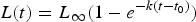 $$L\lpar t \rpar = L_\infty (1-e^{-k\lpar {t-t_0} \rpar })$$
where L ∞ is the asymptote of the function, representing the length of the organism (umbo-to-commissure shell height for bivalves) given infinite time, and k is the growth coefficient in units of years−1. The growth coefficient k is proportional but not equal to the rate of size increase (growth rate): instead, it is an exponential decay constant expressing the rate at which an organism's current size approaches its theoretical maximum or asymptotic size (L ∞). Thus, the larger of two organisms with identical growth coefficient k would grow faster in terms of length per time (Fig. 1). Von Bertalanffy growth parameters L ∞ and k can be readily inferred for a bivalve by measuring the distance between successive annual growth lines/bands (= growth increments) in their cross-sectioned shells. Each dark band (in reflected light) corresponds to an interval of slow shell growth, and these are generally seasonally controlled (e.g., Jones and Quitmyer Reference Jones and Quitmyer1996; Schöne Reference Schöne2008; but see Surge et al. Reference Surge, Lohmann and Dettman2001; Edie and Surge Reference Edie and Surge2013; see also Schoene and Surge [Reference Schoene and Surge2012] on subannual banding). Moss et al. (Reference Moss, Ivany, Judd, Cummings, Bearden, Kim, Artruc and Driscoll2016) found that distance from the equator was positively correlated with life span and inversely correlated with the growth coefficient k, but body size showed no relationship either with latitude or with the other growth parameters. Importantly, only a small proportion of the variation in growth coefficient was explained by latitude; thus, much of the variation in growth coefficient at broad taxonomic scales must be explained by extrinsic or intrinsic variables other than temperature. The degree to which growth rate is constrained by evolutionary history has never been explored in depth, but Moss et al. (Reference Moss, Ivany, Judd, Cummings, Bearden, Kim, Artruc and Driscoll2016) did recover some clustering of growth coefficients within taxonomic orders of bivalves. If closely related species tend to grow at similar rates, it could explain the disjunction between the findings of Moss and colleagues and the studies at narrower taxonomic scopes that recover a stronger dependence of growth rate on environmental conditions. In this study, we use remote-sensing data, a new phylogeny of bivalves, and phylogenetic comparative methods to evaluate the degree to which variation in growth coefficient across Bivalvia can be explained by evolutionary history and environmental variation.
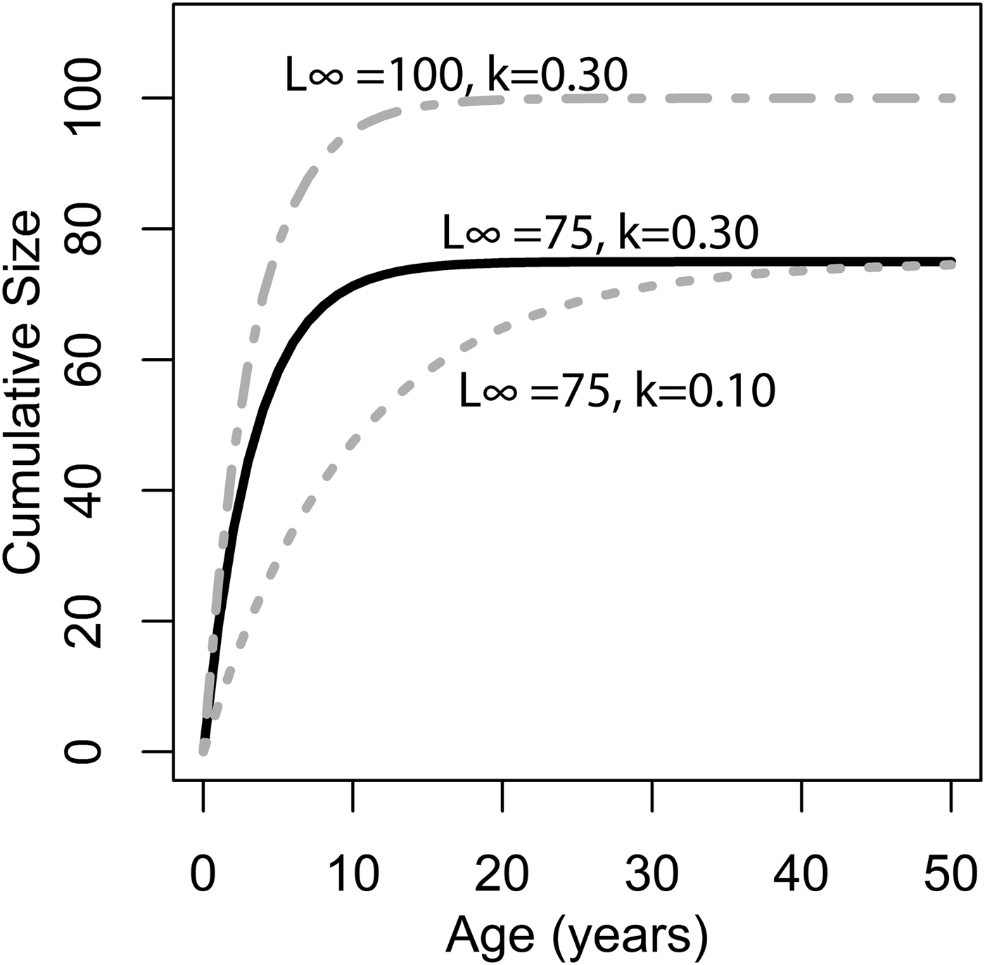
Figure 1. Illustration of changing L ∞ and k of the von Bertlanaffy growth equation (eq. 1). Solid black line: L ∞ = 75, k = 0.30, t 0 = 0. Dashed gray line: L ∞ = 50, k = 0.10, t 0 = 0. Dashed-dotted gray line: L ∞ = 100, k = 0.30, t 0 = 0. k is the rate at which L ∞ is approached. In the scenario of two organisms with identical k values but different L ∞ values (top two lines), the organisms with the higher L ∞ values would accrete more shell in terms of length per time. Alternatively, if L ∞ is identical, but k differs (bottom two lines), then the organisms with the higher k values would accrete more shell in terms of length per time. Thus, direct comparisons between taxa of k in terms of absolute growth rate cannot be made, because L ∞ may different. However, because k is the rate at which L ∞ is approached, it provides information on the growth strategy of the organism in question and may also provide insights into ecology.
Methods
Data Sources
We build on the Moss et al. (Reference Moss, Ivany, Judd, Cummings, Bearden, Kim, Artruc and Driscoll2016) data set to yield 692 observations of life span and the von Bertalanffy parameters k (growth coefficient) and L ∞ (body size) among wild populations of bivalves from the ecological literature. The observations encompass 195 species in 12 orders (Horton et al. Reference Horton, Kroh, Bailly, Boury-Esnault, Brandão, Costello and Gofas2016), with 75 genera represented by multiple species. A complete description of our data set can be found in Moss et al. (Reference Moss, Ivany, Judd, Cummings, Bearden, Kim, Artruc and Driscoll2016). Observations in the Moss et al. (Reference Moss, Ivany, Judd, Cummings, Bearden, Kim, Artruc and Driscoll2016) data set without growth coefficient k are not included in this study.
Deposit feeders have been found to make up a greater proportion of bivalve species at higher latitudes (Berke et al. Reference Berke, Jablonski, Krug and Valentine2014; Edie et al. Reference Edie, Jablonski and Valentine2018), which might influence our results if deposit feeders and suspension feeders differ systematically in their growth parameters or in their responses to temperature or food supply. We acquired data on feeding ecology (i.e., suspension feeding, deposit feeding, or chemosynthetic) from published sources, listing the feeding ecology of congeners when this information was not available for a given species. Suspension feeders comprise 93% of our observations, deposit feeders another 6%, and chemosynthetic bivalves a final 1%. Mean absolute latitude of observations was 48.7° for deposit feeders and 41.9° for suspension feeders.
We use NASA's OceanColor Web, a repository for satellite-based remote-sensing oceanographic data, to obtain data products from the MODIS-Aqua satellite for as many observations in the data set as possible (NASA Goddard Space Flight Center, Ocean Biology Processing Group 2014). Grids of environmental parameters with 1/24-degree spatial resolution (equal to 4.6 km at the equator) are obtained for chlorophyll-a concentration (mg/m3) and sea-surface temperature (SST, °C) for each month between July 2002 and December 2016. This time span does not overlap with every study used in the Moss et al. (Reference Moss, Ivany, Judd, Cummings, Bearden, Kim, Artruc and Driscoll2016) data set (1910–2015, median publication year = 1996). However, the satellite data are assumed to broadly represent oceanic conditions during the original studies; for instance, they encompass five El Niño events, which are major sources of supra-annual variability in the ocean (Philander Reference Philander1989; NOAA Center for Weather and Climate Prediction n.d.). We generate grids of “minimum” and “maximum” values for chlorophyll and SST. Instead of true minima and maxima, which are sensitive to outliers, the values in these grids correspond to the 10th and 90th percentiles of the data in each cell. Results were found to be relatively insensitive to the choice of percentile values (Supplementary Table S1). Environmental predictors are extracted for every available locality in the Moss et al. (Reference Moss, Ivany, Judd, Cummings, Bearden, Kim, Artruc and Driscoll2016) data set.
Most population-level bivalve research is done very close to land, where remote-sensing data are sometimes unavailable. Of the 692 observations in the data set, SST is available for 623 (90%) of them, and chlorophyll-a data for 489 (70%) (Fig. 2). Observations for which only SST is available are distributed fairly evenly, both geographically and phylogenetically. Our data set is biased toward the temperate Northern Hemisphere and toward English-language literature. Four observations from below shelf depths (>200 m) are excluded from comparison with environmental variables, as remote-sensing proxies are unreliable estimates of environmental conditions at great depths. SST and chlorophyll concentration are not correlated with each other in our data set (Supplementary Material 3).
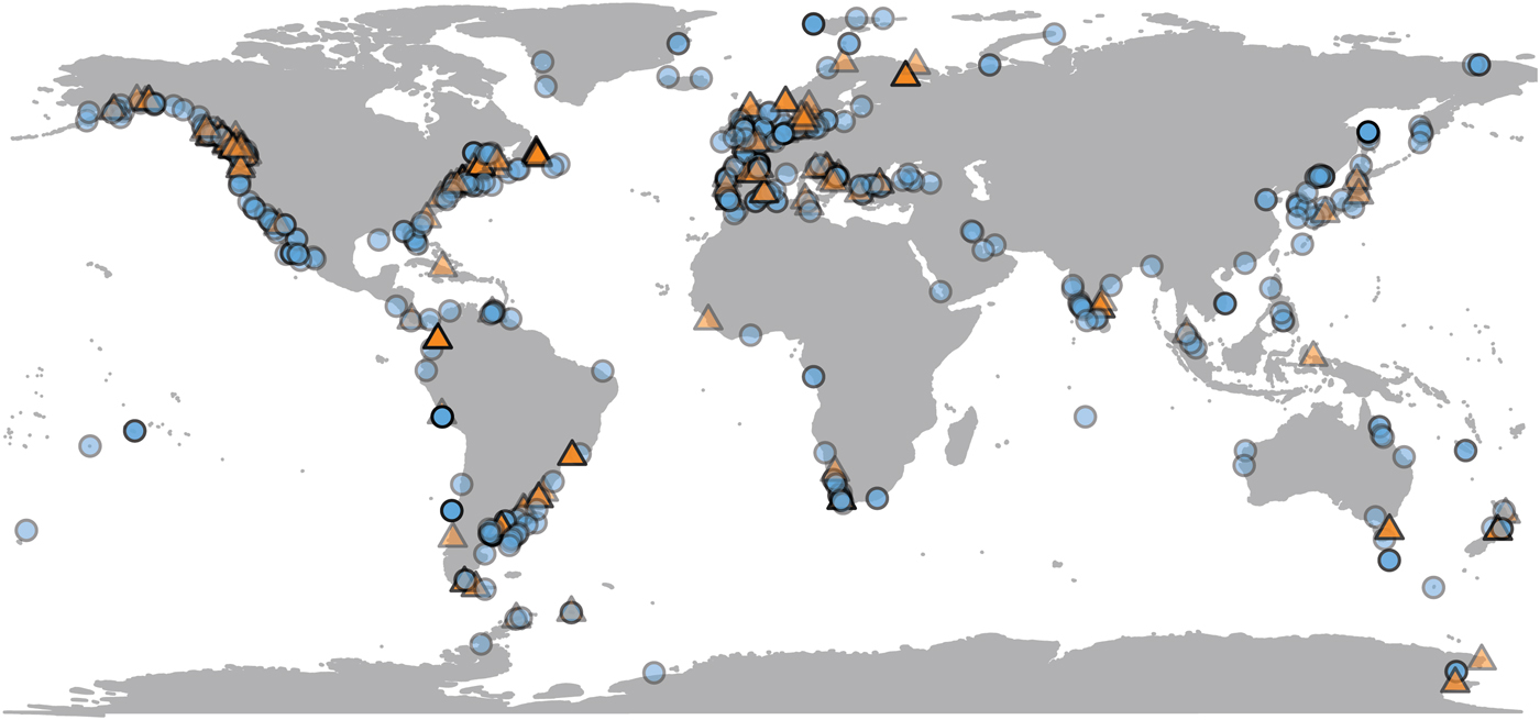
Figure 2. Geographic distribution of growth parameter observations, plotted at 50% opacity. Localities with only chlorophyll or temperature data available are plotted as orange triangles; those with both are plotted as blue circles (see online version for colors). N = 688.
Evaluating Predictors
Growth rate scales exponentially with temperature during the rising phase of a thermal performance curve (Schulte Reference Schulte2015). Because of the close correspondence between growth rate and metabolic rate, we predicted and tested for a linear relationship between SST and the natural log of the growth coefficient. We expected no such exponential relationship between chlorophyll concentration and growth coefficient; instead, growth should increase linearly with food availability, or perhaps as a saturating function reflecting limits on food intake. For this reason, we tested for an association between unlogged chlorophyll concentration and growth coefficient, despite both variables being right skewed and having lower bounds at 0 (Supplementary Material 2). The decision not to log transform either variable does not strongly impact our findings (Supplementary Fig. S3).
Because life-history traits such as growth rate may not show a simple linear response to environmental variables, we use both linear and quantile regression to evaluate predictors of growth rate. Quantile regression estimates the conditional response of a given quantile of a response variable given specified values of predictor variables; in other words, it tests whether certain parts of a response variable regress differently against predictors (Koenker Reference Koenker2013). We use this approach to pursue the apparent relationship between latitude and variability of growth rate across taxa revealed by Moss et al. (Reference Moss, Ivany, Judd, Cummings, Bearden, Kim, Artruc and Driscoll2016: Fig. 3D). To investigate the “shape” of our data, we use a joint test of equality of slopes on the first, second, and third conditional quartiles (the 25th, 50th, and 75th quantiles) of the response variable. Quantile regression is implemented with the ‘quantreg’ package (v. 5.38; Koenker Reference Koenker2013) in R.
Comparing the effects of various environmental parameters on a response variable is less straightforward when data for those parameters are patchy and more complete for some variables than for others. In these cases, it may be hard to separate real differences in predictive power from differences in sample selection. As such, we also evaluate regressions in which we exclude data points for which only temperature is available. We also use a model selection framework to assess the relative importance of taxonomic membership and maximum and minimum values of temperature and chlorophyll as predictors of ln(k) in simple and multiple regressions. This analysis considers only those data points for which both SST and chlorophyll-a concentration are available (N = 472). Finally, we evaluate environment–growth relationships within the 10 most well-sampled families.
Phylogenetic Comparative Methods
To test the robustness of observed correlations and assess the phylogenetic signal of growth rate, we infer a maximum-likelihood phylogeny of bivalve species in the data set using nuclear (18s, 28s) and mitochondrial (COI, 16s) sequence data downloaded from GenBank (Clark et al. Reference Clark, Karsch-Mizrachi, Lipman, Ostell and Sayers2016). Sequence data were available for 135 species (~2.3 sequences per taxon) in 90 genera, represented by a total of 559 observations. Crown Bivalvia probably diverged in the Cambrian to Ordovician (Zong-jie and Sánchez Reference Zong-jie and Sánchez2012; Bieler et al. Reference Bieler, Mikkelsen, Collins, Glover, González, Graf, Harper, Healy, Kawauchi, Sharma, Staubach, Strong, Taylor, Tëmkin, Zardus, Clark, Guzmán, McIntyre, Sharp and Giribet2014); as such, the relatively rapidly evolving molecular markers used here might fail to recover the deepest nodes in the bivalve tree. Consequently, we constrain tree topology at the suborder level, using previously published phylogenies (Bieler et al. Reference Bieler, Mikkelsen, Collins, Glover, González, Graf, Harper, Healy, Kawauchi, Sharma, Staubach, Strong, Taylor, Tëmkin, Zardus, Clark, Guzmán, McIntyre, Sharp and Giribet2014; Combosch et al. Reference Combosch, Collins, Glover, Graf, Harper, Healy, Kawauchi, Lemer, McIntyre, Strong, Taylor, Zardus, Mikkelsen, Giribet and Bieler2017). This constraint tree, our sequence alignment, the phylogeny used in our analyses, and further details on our phylogenetic analysis (Supplementary Data 1) are available in the Supplementary Material.
We calculate Pagel's λ and Blomberg's K, two common measures of phylogenetic signal, for the means of log growth coefficient, log body size, log life span, latitude, and mean observed minimum and maximum SST and chlorophyll concentration using the ‘phytools’ package in R (v. 0.6-60; Revell Reference Revell2012). Pagel's λ is a dimensionless value that expresses the phylogenetic interdependence of trait values: λ = 1 is obtained for traits that are best modeled in a likelihood framework by Brownian motion on a phylogeny with unmodified branch lengths, while lower values indicate that a trait is best modeled by a phylogeny in which internal branch lengths have been shortened relative to terminal branch lengths (Freckleton et al. Reference Freckleton, Harvey and Pagel2002). Blomberg's K is calculated as the variance among species divided by the variance of independent contrasts (Blomberg et al. Reference Blomberg, Garland and Ives2003); the latter is calculated here with 104 simulations. While λ can be no higher than 1, but K can theoretically exceed 1, and values of λ are not directly comparable with values of K. Significance is assessed for K by comparing the observed value against values of K calculated for trait data randomly assigned to the tips of a phylogeny; and significance is assessed for λ using the ratio of the likelihood of the observed phenotypes given the inferred λ to the likelihood of the data given λ = 0. Both metrics are typically used with ultrametric trees (i.e., trees in which the distance from the root to the tip is the same for all tips), so we rescale the phylogeny of bivalves for tests of phylogenetic signal using the chronos function in the ‘ape’ package (v. 5.0; Paradis et al. Reference Paradis, Claude and Strimmer2004). We test phylogenetic signal under three different penalized-likelihood time-scaling settings to assess sensitivity: using a smoothing parameter of 0, and using a smoothing parameter of 1 under either a relaxed or correlated model of molecular evolution.
Observed organismal growth coefficient reflects both a heritable reaction norm—the curve describing response to environmental variation—and environmental conditions (David et al. Reference David, Gibert, Moreteau, DeWitt and Scheiner2004). For this reason, we calculate the phylogenetic signal of not only the mean growth coefficient observed, but also of the maximum, and we hypothesize that this might more accurately reflect the growth reaction norm.
Phylogenetic generalized least squares (PGLS) is used to evaluate the same relationships treated with linear regression while accounting for phylogenetic autocorrelation in the context of the phylogeny inferred in this study. For this analysis, mean trait values are used to evaluate minimum and maximum chlorophyll concentration and SST as predictors of the log of growth coefficient, and Akaike weights are compared for simple and multiple regression models. This analysis uses only those observations for which both temperature and chlorophyll data are available, resulting in a data set of 121 species. PGLS uses information about the phylogenetic signal (Pagel's λ) of residuals to scale the off-diagonals of the variance–covariance matrix used in the regression; our analysis uses a maximum-likelihood estimate of this parameter. All PGLS analyses use a phylogeny time-scaled with the chronos function in the ‘ape’ R package, with a smoothing parameter of 0. All R code associated with this study is provided in the Supplementary Material and was run in v. 3.5.0. (2018-04-23; R Core Team 2013).
Results
Regressions
Environmental predictors generally only weakly predict growth coefficient k (Fig. 3). All environmental parameters besides maximum chlorophyll concentration regress significantly against k, but with low r 2 values: minimum SST, the strongest predictor, explains 12.2% of the variation in log growth coefficient, while maximum SST explains 7.2%. Minimum chlorophyll concentration explains 1.1% of the variation in unlogged growth coefficient. Multiplying k by L ∞ gives a response variable that should conform more closely to true growth rate in distance per time, but this response variable shows weaker or comparable relationships with all predictors (Supplementary Fig. S2). Excluding non–suspension feeding bivalves has a negligible effect on the strength of the predictors under study, including chlorophyll-a concentration (Supplementary Table S2). SST is available for 20% more of the observations in the data set, but excluding these data also has little impact on our findings: r 2 values for the regressions of ln(k) against minimum and maximum SST is nearly identical when SST-only observations are removed (0.117 and 0.080, respectively).
Figure 3. Linear regression and quantile regression plotted for minimum and maximum temperature and chlorophyll-a concentration. The 5th, 25th, 75th, and 95th conditional percentiles of the response variable are shown as dashed lines. Tests of equality of slopes reveal that only maximum temperature is associated with a change in the spread of growth coefficient (Supplementary Data 4). Sample sizes and coefficients of determination are shown for each regression. Sample sizes are identical for minimum and maximum predictors. *p < 0.05; ***p < 0.0005.
Quantile regression reveals that the growth coefficient is slightly more variable at higher maximum but not minimum SST. Increasing chlorophyll concentration is not significantly associated with a change in the spread of growth coefficients (Fig. 3, Supplementary Table S3). Joint tests of equality of slopes reveal that the first, second, and third conditional quantiles are significantly different for maximum but not minimum temperature. Increased spread of observed growth coefficient is therefore associated with high maximum but not high minimum annual temperature. Joint tests of equality of slopes return insignificant results for quantiles conditional on chlorophyll-a concentration.
Regression models in which taxonomic family membership is included as a categorical predictor receive uniformly high Akaike information criterion (AIC) scores relative to those that include only environmental predictors, such that the Akaike weights (AICw) of models that include family summed to ~1 (Table 1). The best-supported model includes family and minimum SST and chlorophyll a (AICw = 0.7916), with some support for models including minimum and maximum SST and chlorophyll and family (AICw = 0.1587) and including minimum SST and family (AICw = 0.04965). Regressions that include family membership and at least one environmental variable have the highest r 2 value (>0.35), and r 2 for the regression including only family membership (0.3062) is higher than any that include only environmental variables. In a few cases, environment–growth coefficient regressions within subclades are stronger than those that include the entire data set (Supplementary Fig. S4). Among the top 10 best-sampled families, relatively high r 2 values are observed for the regression between SST and ln(k) among the Veneridae (r 2 = 0.33, N = 125) and the Pectinidae (r 2 = 0.30, N = 81). Neither the number of observations of a taxonomic family nor the standard deviation of observed environmental values predicts the strength of the environment–k regression within that family.
Table 1. Model support and effect sizes (adjusted r 2) in linear regressions and phylogenetic generalized least squares (PGLS). Model with the highest Akaike information criterion (AIC) score shown in bold. A, AIC, ΔAIC, Akaike weights, and r 2 values for simple and multiple regressions with environmental variables and family membership as predictors. Only includes observations with sea-surface temperature (SST) and chlorophyll data (N = 550). B, Model support and effect size for PGLS. Only incorporates observations with corresponding tips in our phylogeny and with SST and chlorophyll data. Sample size is N = 136 species.

Phylogenetic Comparative Methods
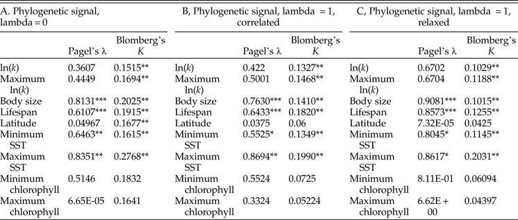
Tests of phylogenetic signal show that growth coefficient is somewhat conserved within lineages across Bivalvia, although not to the degree that body size and life span are (Table 1). For growth coefficient, all estimates of Pagel's λ are intermediate (between 0.3 and 0.7) but statistically insignificant, indicating that residuals in the fitted models are adequately modeled as being independent. On the other hand, all estimates of Blomberg's K are statistically significant and comparable in magnitude to estimates for body size and life span (K = 0.10–0.14), meaning that phylogenetic information helps predict the observed growth coefficient data. λ and K perform best under different models of trait evolution (Münkemüller et al. Reference Münkemüller, Lavergne, Bzeznik, Dray, Jombart, Schiffers and Thuiller2012), so rather than being contradictory, these findings indicate that growth coefficient is somewhat conserved within lineages. Latitude and log chlorophyll concentration take mostly low values of both metrics of phylogenetic signal, but SST exhibits high phylogenetic signal comparable with body size and life span. Different approaches to reconstructing the timescale of bivalve evolution produce concordant estimates of phylogenetic signal in terms of their relative ordering and their statistical significance, except in the case of latitude. Phylogenetic signal is slightly higher for the maximum growth coefficient observed within species than for the mean value in all cases, consistent with our earlier suggestion that the maximum k observed within a species should more closely reflect the heritable component of growth coefficient; however, the difference is slight. Some groups of bivalves show highly conserved values of one or more growth parameters (Fig. 4): Hiatellidae, the family including the geoduck Panopea, is characterized by long life spans, moderately high L ∞, and fairly low growth coefficients, while the razor clams (Pharidae, including Ensis and Siliqua) are relatively large (in terms of maximum dimension), have intermediate life spans, and grow at variable rates.

Figure 4. Maximum-likelihood phylogeny of 135 bivalve species, time-scaled using penalized likelihood. Branch lengths correspond to time, but because our downstream analyses depend only on the relative timing of divergences rather than on absolute dates, the geological timescale is not shown here. Growth coefficient, body size, and life span are shown for each species. Colors (see online version) correspond to values on a log scale.
Multiple regression in a PGLS framework uncovers environment–growth relationships that are broadly similar in their effect sizes and relative ordering to those returned by nonphylogenetic regressions (Table 1). Models including only minimum or maximum chlorophyll as predictors have effectively no support. Maximum-likelihood estimates of Pagel's λ, which in PGLS models the phylogenetic signal of residuals, are low to intermediate across all models. When the value of λ is set to 1, a handful of observations in the Veneridae drive the effect size for all minimum temperature–growth coefficient relationships above r 2 = 0.4 (Supplementary Table S4), recapitulating the point made by Uyeda et al. (Reference Uyeda, Zenil-Ferguson and Pennell2018) that phylogenetic comparative methods are no less vulnerable to outliers than traditional comparative approaches.
Discussion
Environmental Predictors of Growth Coefficient
SST is consistently a stronger predictor of growth coefficient than chlorophyll-a concentration in all of our analyses. Although the link between metabolic rate and shell growth rate is indirect (Lewis and Cerrato Reference Lewis and Cerrato1997; Pouvreau et al. Reference Pouvreau, Bourles, Lefebvre, Gangnery and Alunno-Bruscia2006; Bourlès et al. Reference Bourlès, Alunno-Bruscia, Pouvreau, Tollu, Leguay, Arnaud, Goulletquer and Kooijman2009), as is the link between shell growth rate and growth coefficient (see discussion in “Methods”), the well-documented and theoretically robust temperature dependence of metabolism probably explains our results (Gillooly et al. Reference Gillooly, Brown and West2001). Seafloor temperature tends to correspond more closely with SST during the winter than during the summer (Prandle and Lane Reference Prandle and Lane1995; Austin et al. Reference Austin, Cage and Scourse2006), which may explain why minimum temperature is the strongest predictor in our analyses. Moss et al. (Reference Moss, Ivany, Judd, Cummings, Bearden, Kim, Artruc and Driscoll2016) found that the standard deviation of all k observations within a latitudinal bin decreased from the equator to the poles; along the same line, our results offer some support for the idea that higher temperatures are associated with not just higher k but also a greater spread of k. The link between metabolic rate and growth coefficient is highly indirect: not all of the energy produced by metabolism is devoted to shell growth, and there are important differences between growth rate and growth coefficient (see “Methods”). However, a latitudinal gradient in not just the mean but also the spread of metabolic rates would have wide-reaching evolutionary implications. If temperature increases the maximum metabolic rate possible without a comparable increase in the minimum, then the pace of life set by metabolism is not simply higher in the tropics: instead, the tropics facilitate a wider range of metabolic rates, and perhaps by extension, a wider range of lifestyles. This scenario provides a plausible mechanism for the latitudinal gradient in functional diversity (Stuart-Smith et al. Reference Stuart-Smith, Bates, Lefcheck, Duffy, Baker, Thomson, Stuart-Smith, Hill, Kininmonth, Airoldi, Becerro, Campbell, Dawson, Navarrete, Soler, Strain, Willis and Edgar2013; Edie et al. Reference Edie, Jablonski and Valentine2018), although the links between growth coefficient, growth rate, and metabolic rate are not sufficiently understood at present to speculate further.
The apparent unimportance of food supply in determining spatial patterns in growth coefficient might be a biologically meaningful result, but there are several issues with interpreting it at face value. Chlorophyll concentration shows strong spatiotemporal variability below the ~5 km, month-scale resolution captured by the MODIS-Aqua satellite (Mackas et al. Reference Mackas, Denman and Abbott1985; Wambeke et al. Reference Wambeke, Heussner, Diaz, Raimbault and Conan2002). Not all surface primary production reaches the seafloor, which might further impact the accuracy of this predictor. In short, imperfections of the satellite proxy might obscure a truly strong relationship between primary production and bivalve growth coefficient. This would be consistent with results from laboratory and in situ studies, which typically recover phytoplankton concentration as a strong predictor of bivalve growth rate in terms of distance over time (Beukema and Cadee Reference Beukema and Cadee1991; Savina and Pouvreau Reference Savina and Pouvreau2004; Bourlès et al. Reference Bourlès, Alunno-Bruscia, Pouvreau, Tollu, Leguay, Arnaud, Goulletquer and Kooijman2009; Gosling Reference Gosling2015a), and with paleontological research that suggests primary production is a driver of changes in growth coefficient over deep time (Haveles and Ivany Reference Haveles and Ivany2010). Aside from the possibility that the satellite chlorophyll-a proxy might not closely reflect in situ conditions, those in situ conditions might not be the ones that matter most to bivalves. Diatom abundance, for example, could be a stronger control on bivalve growth than the concentration of phytoplankton in general (Gosling Reference Gosling2015a). Similarly, dissolved organic matter and non-phytoplankton particulate organic matter, neither of which are reflected by our predictors, are important components of the diets of some bivalves (Kang et al. Reference Kang, Sauriau, Richard and Blanchard1999; Gosling Reference Gosling2015b). Particulate organic matter may be an especially important component of marine food webs at high latitudes (Peck et al. Reference Peck, Barnes and Willmott2005; Mincks and Smith Reference Mincks and Smith2007).
Other lines of evidence support our finding that food supply is weakly associated with growth coefficient at best. McClain et al. (Reference McClain, Allen, Tittensor and Rex2012) reported that depth, a proxy for food availability, did not correlate with growth rate or per-mass metabolic rate among a wide variety of marine organisms after accounting for covariation with body size and temperature, corroborating previous work (Childress Reference Childress1995). Instead, the authors found that food availability controls biomass, abundance, and diversity in marine communities. Killam and Clapham (Reference Killam and Clapham2018) recovered a similar pattern despite using a different kind of data: chlorophyll-a concentration showed no relationship with the occurrence of seasonal cessations in bivalve shell growth, which influence long-term growth (Gosling Reference Gosling2015a). Even if growth coefficients were expected to depend on food supply, growth should be more sensitive to changes in temperature: the Arrhenius equation predicts that the rate at which aerobic metabolism (or any chemical reaction) proceeds should scale exponentially with temperature (Schulte Reference Schulte2015), whereas growth rate would be at most expected to scale linearly with the amount of food ingested. Growth coefficient is an imperfect proxy for growth rate in terms of size increase per time, but our finding that chlorophyll concentration shows little or no relationship with the product of k and L ∞ (Supplementary Fig. S2) argues against the possibility that chlorophyll concentration controls growth rate but not growth coefficient. While our results do not preclude a role for food supply in controlling growth rate and metabolic rate, they do support temperature as a more important determinant of spatial patterns in growth parameters, consistent with previous findings (Heilmayer et al. Reference Heilmayer, Brey and Portner2004; Killam and Clapham Reference Killam and Clapham2018). Notably, one of the only bivalve groups above the species level in which a strong temperature–growth relationship has been demonstrated is the Pectinidae (Heilmayer et al. Reference Heilmayer, Honnen, Jacob, Chiantore, Cattaneo-Vietti and Brey2005), and in our data set the log of growth coefficient regresses against SST with a relatively high r 2 (0.30) in this group (Supplementary Fig. S4). Why the dependency of growth rate on environmental conditions should vary so much between taxa is not immediately clear, but it is consistent with our finding that evaluating environmental predictors in a PGLS framework does not result in appreciably greater effect sizes.
Importantly, no environmental predictor or combination of predictors explains more than 15% of the variation in log growth coefficient across Bivalvia. Because this remains so even when considering environment–growth relationships in a PGLS framework, we infer that “phylogenetic inertia” does not explain the weak dependency of growth coefficient on broad-scale environmental conditions observed in our data set. In other words, it does not appear to be the case that environment–growth relationships become weaker at deeper nodes in the tree, at least at the broad phylogenetic scale considered in this analysis. Our finding that effect sizes of environment–growth regressions within bivalve families are not consistently greater than those across all Bivalvia supports this inference (Supplementary Fig. S4). Conceivably, further study within subclades—for example, within the Veneridae or the Pectinidae (Supplementary Fig. S4)—might recover stronger environment–k relationships or might reveal interesting k– L ∞ interactions not seen in our study. Some of our results could be peculiar to the coarse phylogenetic and geographic scale of our study, but a finer investigation is not possible with the data at hand. Environmental parameters do not appear to explain much of the variation in growth coefficient at any taxonomic scale.
Beyond the imperfections in the environmental proxies mentioned previously, the poor environment–growth correspondence we observe can probably be attributed in part to metabolic rate compensation, the suite of biochemical processes by which organisms modulate their metabolic rates independently of environmental conditions (Bullock Reference Bullock1955). For example, a near-independence of temperature and the energy available for growth across a limited temperature range was observed by Widdows (Reference Widdows1978) and Sobral and Widdows (Reference Sobral and Widdows1997) for the mussel Mytilus edulis and the venerid clam Venerupis philippinarum, respectively, and in both cases was attributed to metabolic rate compensation.
Evolution of Growth
Although phylogenetic inertia might not explain why studies of environmental determinants of growth at broad taxonomic scales fail to recapitulate the results of within-species experimental research, conservation of growth coefficient within lineages does appear to be a real phenomenon. This is indicated on the one hand by the moderate phylogenetic signal recovered for k in this study (Table 2). On the other hand, and perhaps more compelling, is the observation that family membership alone predicts growth coefficient more successfully than any combination of environmental variables (Table 1). These findings corroborate Moss et al. (Reference Moss, Ivany, Judd, Cummings, Bearden, Kim, Artruc and Driscoll2016) and Dexter and Kowalewski (Reference Dexter and Kowalewski2013), who showed that bivalves within the same taxonomic families and orders typically had similar growth coefficients.
Table 2. Results of tests of phylogenetic signal. We performed 1000 simulations for each test of Blomberg's K; as such, the synthetic p-values associated with that test cannot go below 0.001. A, Phylogenetic signal calculated on an ultrametric tree scaled with the assumption of a strict molecular clock. B, The same, calculated on a tree time-scaled assuming autocorrelated but variable rates of molecular evolution. C, The same, calculated on a tree time-scaled under a relaxed model of molecular evolution. SST, sea-surface temperature. *p ≤ 0.05; **p ≤ 0.005; ***p ≤ 0.0005.
Growth coefficient itself might be subject to phylogenetic inertia, but it is worth considering whether growth is instead a function of phylogenetically conserved environmental conditions. Tests of phylogenetic signal reveal that closely related bivalves might show a weak tendency to live at similar latitudes (Table 2), although other studies have recovered stronger tendencies of this kind (Tomašových and Jablonski Reference Tomašových and Jablonski2016). More compellingly, environmental temperature exhibits relatively high phylogenetic signal, and some of the highest values of λ and K in our analysis are obtained for maximum SST. If close relatives tend to live at similar temperatures, we might not need to invoke phylogenetic conservation of growth coefficient to explain some of the patterns recovered in this study. Other sorts of ecological similarity among closely related taxa might also explain some of the phylogenetic conservatism of growth coefficient observed here. For example, the slow-growing geoducks (Panopea) share a deep-burrowing lifestyle (Kondo Reference Kondo1987); likewise, the cementing ostreids (Ostrea, Crassostrea) share a generally high growth coefficient. However, there is some independent evidence to support a scenario in which growth trajectories are phylogenetically conserved independent of environmental conditions. Vladimirova et al. (Reference Vladimirova, Kleimenov and Radzinskaya2003) measured metabolic rates at a standardized temperature (20°C) across Bivalvia and found some conservation of rates within orders and families. In that study, bivalves living closer to the equator exhibited higher metabolic rates when acclimatized to and measured at a standard temperature. In conjunction with the findings of the present study, this experimental finding indicates that the higher rates of growth and metabolism seen in the tropics are the result not just of phenotypically plastic responses to environmental gradients, but also of changes in the heritable reaction norms of growth rate and metabolic rate.
Conclusions
Fossilized growth rates are one of the best and most widely available proxies for studying the history and evolution of metabolic rates, though they have rarely been used for this purpose. Our study calls attention to some important considerations for the use of growth coefficients in this research effort. At the relatively broad spatial, environmental, and taxonomic scales considered in this study, SST explains only about one-tenth of the variation in growth coefficient, and surface chlorophyll-a concentration accounts for almost none. Multiple regression and tests of phylogenetic signal indicate that closely related bivalves grow at similar rates. The conflict between our results and those of previous within-species studies may be explained in part by shortcomings of remote-sensing proxies. Taxonomic membership is a good predictor of growth coefficient, but a substantial portion of the variation in growth coefficient must be explained by fine-scale environmental conditions or by intrinsic processes like metabolic rate compensation. Studies of environmental or temporal variation in growth rate, growth coefficient, or metabolic rate that do not consider phylogeny or do not restrict analysis to within-lineage changes risk discovering only spurious pattern. Intuitively, an oyster k is not a geoduck k is not a scallop k.
Because no temporal trend in growth rate through the Phanerozoic has been established, it is unclear what the apparently weak dependence of growth coefficient on chlorophyll concentration implies for the hypothesis that increased nutrient availability is responsible for trends in body size through deep time (Bambach Reference Bambach1993). However, our study provides evidence against a scenario in which increased nutrient availability through the Phanerozoic promoted larger body sizes by enabling metazoans to grow faster. Instead, increased nutrient availability probably influenced ecosystem structure (Knoll and Follows Reference Knoll and Follows2016; but see McClain et al. Reference McClain, Heim, Knope and Payne2018) and patterns of diversity (Martin Reference Martin1996; McClain et al. Reference McClain, Allen, Tittensor and Rex2012; but see Hunt et al. Reference Hunt, Cronin and Roy2005), at least in the oceans.
Outstanding questions include: To what degree are our findings particular to bivalves? Can some of the substantial variation in growth coefficient that is not explained by remote-sensing predictors be attributed to fine-scale environmental variation? How robust is the apparent latitudinal gradient in the variability of growth coefficient, and does this map onto a similar gradient in metabolic rate? More generally, what are the long-term trends in growth rate and metabolic rate, and how do they relate to the evolution of body size over the Phanerozoic? Resolving these uncertainties will require the integration of data with a broader taxonomic scale from experimental physiology, sclerochronology, macroecology, and the fossil record.
Acknowledgments
This work was funded by a Rackham Merit Fellowship (J.S.) and a David and Lucile Packard Fellowship (S.F.).


 Open access