


INTRODUCTION
Iceberg calving is responsible for about one third of average annual mass loss from Antarctic ice shelves, with the remainder being due to basal melting (Liu and others, Reference Liu2015). Calving is a complex process and the quest for a unified calving law continues to this day (Bassis, Reference Bassis2011; O'Leary and Christoffersen, Reference O'Leary and Christoffersen2013), increasing uncertainty in diagnostic and prognostic ice-sheet simulations (e.g. Nick and others, Reference Nick, van der Veen, Vieli and Benn2010; Bassis, Reference Bassis2011; Bassis and Jacobs, Reference Bassis and Jacobs2013; DeConto and Pollard, Reference DeConto and Pollard2016). The formation and propagation of rifts or fractures is a precursor of iceberg calving from and the disintegration of Antarctic ice shelves (Scambos and others, Reference Scambos, Hulbe, Fahnestock and Bohlander2000; Fricker and others, Reference Fricker, Young, Coleman, Bassis and Minster2005a, Reference Fricker, Bassis, Minster and MacAyealb; Bassis and others, Reference Bassis, Coleman, Fricker and Minster2005, Reference Bassis2007, Reference Bassis, Fricker, Coleman and Minster2008; Glasser and Scambos, Reference Glasser and Scambos2008; Hulbe and others, Reference Hulbe, LeDoux and Cruikshank2010; Jansen and others, Reference Jansen2010, Reference Jansen2015; McGrath and others, Reference McGrath2012a, Reference McGrathb; Luckman and others, Reference Luckman2012; Borstad and others, Reference Borstad2012, Reference Borstad, Rignot, Mouginot and Schodlok2013; Kulessa and others, Reference Kulessa, Jansen, Luckman, King and Sammonds2014; Walker and others, Reference Walker, Bassis, Fricker and Czerwinski2015). It is not usually possible to ascribe a single factor to a rift propagation event; instead it is more likely that rift propagation occurs when there is an imbalance between the governing environmental parameters, where each parameter is subject to change in space and time (Fricker and others, Reference Fricker, Young, Coleman, Bassis and Minster2005a, Reference Fricker, Bassis, Minster and MacAyealb; Bassis and others, Reference Bassis, Coleman, Fricker and Minster2005, Reference Bassis2007, Reference Bassis, Fricker, Coleman and Minster2008; Glasser and Scambos, Reference Glasser and Scambos2008).
Previous work focused on elucidating the controls exerted by selected environmental parameters on rift propagation such as, atmospheric temperature, winds, tides, sea-ice fraction, tsunamis, ocean circulation or mélange within ice shelf rifts, although an approach that evaluates their combined effects is currently not available (Fricker and others, Reference Fricker, Young, Coleman, Bassis and Minster2005a, Reference Fricker, Bassis, Minster and MacAyealb; Bassis and others, Reference Bassis, Coleman, Fricker and Minster2005, Reference Bassis, Fricker, Coleman and Minster2008; Nick and others, Reference Nick, van der Veen, Vieli and Benn2010; Walker and others, Reference Walker, Bassis, Fricker and Czerwinski2015). In the most comprehensive analysis of environmental controls on rift propagation to date, Bassis and others (Reference Bassis, Fricker, Coleman and Minster2008) were unable to identify a statistically-significant environmental forcing-response relationship owing to the short observation period. Insufficient understanding of such indirect relationships thus drives the need for an integrated statistical framework that can identify and quantify predictable forcing-response relationships from observable environmental parameters (Bassis and others, Reference Bassis2011; Bassis and Jacobs, Reference Bassis and Jacobs2013).
Here we describe a statistical network approach derived from Systems Analysis that shows promise in evaluating complex glaciological processes, and provide an initial demonstration of the approach by applying it to a large tabular iceberg calving event on the Amery Ice Shelf, East Antarctica (Fig. 1).

Fig. 1. MODIS Mosaic of Antarctica (MOA) image of the Amery Ice Shelf in 2009 (Scambos and others, Reference Scambos, Haran, Fahnestock, Painter and Bohlander2007; Haran and others, Reference Haran, Bohlander, Scambos, Painter and Fahnestock2014). (a) Locations of the Amery Ice Shelf in Antarctica (inset), the ‘Loose Tooth’ (dashed box) and the G3 AWS. (b) Close-up of the ‘Loose Tooth’ within the dashed box shown in (a), with transverse (T1, T2) and longitudinal (L1, L2) rifts labelled according to previous nomenclature (Fricker and others, Reference Fricker, Young, Coleman, Bassis and Minster2005a, Reference Fricker, Bassis, Minster and MacAyealb; Bassis and others, Reference Bassis, Coleman, Fricker and Minster2005, Reference Bassis2007, Reference Bassis, Fricker, Coleman and Minster2008).
SYSTEMS ANALYSIS
Introduction
Falling within the domain of Systems Thinking, Systems Analysis has been used in business and engineering for more than 30 years to identify systematic patterns of behaviours between directly and indirectly related processes, based on influence diagrams and Bayesian network analyses of inherent uncertainties (e.g., Kirkwood, Reference Kirkwood1998; Kjaerulff and Madsen, Reference Kjærulff and Madsen2008). Systems Analysis can also evaluate causes and effects of processes in the human brain (Penny and others, Reference Penny, Stephen, Michelli and Friston2004), cybernetics (Wiener, Reference Wiener1961; Bateson, Reference Bateson1979), supply chain risk assessments (Ghadge and others, Reference Ghadge, Dani, Chester and Kalawsky2013), social systems theories (Buckley, Reference Buckley1968; Luhmann, Reference Luhmann1996, Lang and De Sterck, Reference Lang and De Sterck2012) and ecological modelling (Boerlijst and others, Reference Boerlijst, Oudman and de Roos2013). Although Systems Analysis has rarely been applied to cryospheric problems, it shows promise in evaluating causes and effects of complex glaciological processes from in situ data (e.g. Boyd, Reference Boyd2001).
Systems Analysis considers sequences of events (e.g., sequential bursts of rift propagation during an iceberg calving event) and their causes (e.g. interacting ice-dynamic, ocean and atmospheric forcings) as inherently inter-related rather than isolated (Kirkwood, Reference Kirkwood1998). Even though measurements may have been made disparately in space and time and with different instrumentation, the data are considered as inter-related through the observed process, such as, a calving event. Methods of Systems Analysis were traditionally classified as either hard or soft. Hard systems are those dominated by deterministic relationships that can be captured by numerical or computer modelling (Checkland, Reference Checkland1981). Soft systems are less easily quantified and include behavioural or expressional values, such as influence, opinion and qualitative dimensions in the system structure (Checkland and Scholes, Reference Checkland and Scholes1990). In the interest of computational efficiency, it is common practice to implement empirically-based calving laws in ice-sheet models, which are statistical in nature and less representative of the actual physics of fracture (Bassis, Reference Bassis2011). Many such laws exist and the analyst or modeller must make a choice, based on an appreciation of the glaciological environment to be simulated. Because the deterministic power of statistical calving laws is therefore compromised (Bassis, Reference Bassis2011), a combination of hard system and soft system techniques is required in evaluating calving processes – commonly known as an Evolutionary Systems approach (Checkland, Reference Checkland1981; Checkland and Scholes, Reference Checkland and Scholes1990; Banathy, Reference Banathy1998).
Current approach: systems dynamics
Systems Dynamics is a commonly used technique of Systems Analysis that is well suited for application to environmental problems (Forrester, Reference Forrester and De Greene1993; Kirkwood, Reference Kirkwood1998). Systems Dynamics considers a ‘V’-style model (Fig. 2) that consists sequentially of System Specification (a logical representation that captures the complex system's structure from observable parameters), System Architecture (developing an appreciation of the system behaviour, in this case through reconciliation of statistical relationships between the governing parameter trends and outliers to generate a predictor chain), System Design and Integration (a scalable conceptual System Model designed to represent the physical system based on the observable parameters) and System Validation and Verification (diagnostic and prognostic model runs) (Forrester, Reference Forrester and De Greene1993). In support of both System Validation and Verification two types of sensitivity analysis were carried out, including (1) an initial ‘error-check’ modelling run that used variance multipliers to ascertain output confidence and (2) a later appraisal of variance in the input to output response to ascertain predictor-response relationships.
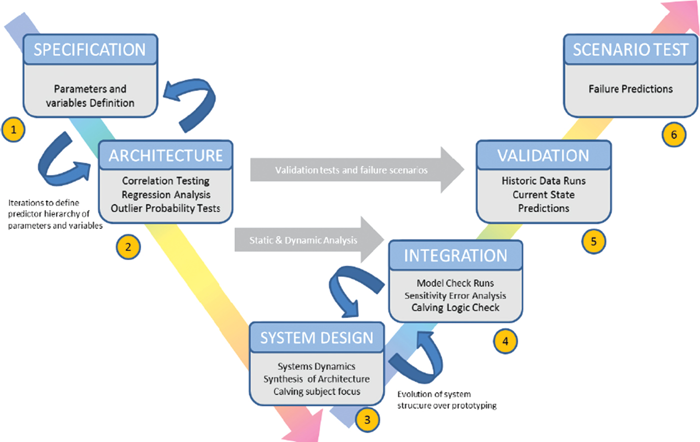
Fig. 2. The Systems Analysis V-model as adapted to the Amery ‘Loose Tooth’ rift system.
To provide an initial demonstration of Systems Analysis of a complex calving event, we apply it to the large nascent iceberg on the Amery Ice Shelf colloquially known as the ‘Loose Tooth’ (Fig. 1; Fricker and others, Reference Fricker, Young, Allison and Coleman2002, Reference Fricker, Young, Coleman, Bassis and Minster2005a, Reference Fricker, Bassis, Minster and MacAyealb; Bassis and others, Reference Bassis, Coleman, Fricker and Minster2005, Reference Bassis2007, Reference Bassis, Fricker, Coleman and Minster2008; Walker and others, Reference Walker, Bassis, Fricker and Czerwinski2015). We provide a step-by-step description of the V-model application to the ‘Loose Tooth’ in the section Application of Systems Analysis to Amery ‘Loose Tooth’, with specific reference to the V-model illustrated in Figure 2.
APPLICATION OF SYSTEMS ANALYSIS TO AMERY ‘LOOSE TOOTH’
System specification
The System specification (i) specifies the parameters of interest, i.e. ‘Loose Tooth’ geometry and potential atmospheric and glaciological forcings; and (ii) defines the logic model for potential interactions between these forcings and the effects on ‘Loose Tooth’ evolution. The specification is driven by the design requirements that are provided in two forms, system requirements and performance requirements.
System requirements
The system requirements include a logical framework of parameters and deliberately coarse data, typifying many in-situ glaciological datasets from remote locations while simplifying the demonstration of the Systems Analysis approach (Table 1). Environmental data were taken from the permanent G3 Automated Weather Station (AWS), located at 70°53′26″S 69°52′14″E on the Amery Ice Shelf 300 km upstream of the ‘Loose Tooth’. Two other weather stations, AM01 and AM02, are in closer proximity to the ‘Loose Tooth’, however they only acquired data from 2002 to 2006 (AM01) and 2001–07 (AM02) and not used in our full 10-year modelling window. It is recognised that to approximate system relationships, the pattern of behaviour between variables is more important in identifying predictor relationships than the consideration of absolute values of individual variables. The assumption is then made that while the variable value at the rift tip will differ from the variable value at the G3 AWS, given the geographical proximity the relative trends (if not the absolute magnitude) will be sufficiently comparable for the analysis to be valid.
Table 1. List of environmental parameters used in this study, including metadata. The data from the Amery G3 weather station are available online at http://aws.acecrc.org.au/datapage.html
The weather station data include the following parameters, all averaged over 1 year for a 10-year period from 1998 to 2008; air temperature (T), subsurface temperature (SST), air pressure (Pa), relative humidity (RH), wind direction (WVD), wind magnitude (WVM) and net snow accumulation (AC). Ice-shelf thickness (TH) and rift lengths (T1, T2) are derived from reports from the Amery Ice Shelf (Bassis and others, Reference Bassis, Coleman, Fricker and Minster2005, Reference Bassis2007, Reference Bassis, Fricker, Coleman and Minster2008). This is justified in that the thickness change of much of the Amery Ice Shelf, including our study area, was effectively negligible (<<5 m) on the timescale of a decade between 1994 and 2012 (Paolo and others, Reference Paolo, Fricker and Padman2015).
The logical framework (Fig. 3) is based on the flow diagram of Glasser and Scambos (Reference Glasser and Scambos2008, their Fig. 8) of relationships between atmospheric, oceanic and glaciological factors that affected the progressive disintegration of the Larsen B Ice Shelf. The framework is adapted to describe the anticipated forcing-response relationships between the environmental parameters governing the propagation of rift T2 (km) (Fig. 4). That rift is critical for ‘Loose Tooth’ detachment and accordingly is particularly well studied (e.g., Bassis and others, Reference Bassis, Coleman, Fricker and Minster2005, Reference Bassis2007, Reference Bassis, Fricker, Coleman and Minster2008).
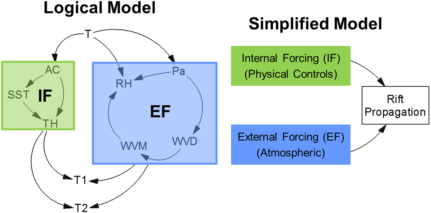
Fig. 3. Full (left) and simplified (right) logical models of internal forcings (IF) and external forcings (EF) for the Amery ‘Loose Tooth’ rift system, as adapted from the Glasser and Scambos (Reference Glasser and Scambos2008) influence map for Antarctic ice-shelf collapse. See Table 1 for a description of the parameters and their abbreviations.
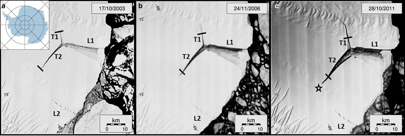
Fig. 4. Sequence of MODIS images tracking the Amery ‘Loose Tooth’ rifts in the austral summers of (a) 2003/04, (b) 2006/07 and (c) 2011/12; see images for exact dates (http://nsidc.org/data/iceshelves_images/index_modis.html). Solid lines mark the reference positions for the rift tips in 2003, and the star in (c) marks the projected maximum lengths that T2 and L2 (~25 km) can attain before T2 and L2 intersect and the nascent ‘Loose Tooth’ iceberg detaches in our system model.
Performance requirements
The performance requirements are provided in the form of a detachment criterion, which is identified from both a hypothesized maximum T2 length criterion and a detachment probability. Following Bassis and others (Reference Bassis2007) we fix T2′s maximum-length criterion at 25 km before detachment will occur, either as a consequence of T2 intersecting with L2 or an equivalent critical event (Fig. 1c). We emphasize that L2 is not explicitly included in our model, assuming instead that L2 will continue to propagate at the same rate as T2.
Bassis and others (Reference Bassis2007; their Fig. 12) showed that the minimum stress required for propagation decreases exponentially with rift length. On the assumption that rift propagation probability (RP) scales inversely with minimum stress, we can therefore assign a nominal value of RP (in units of %) to each value of T2 rift length (km) from a logarithmic fit to the data (solid black line in Fig. 5), yielding
 $$RP = 15.7\ln (T2) + \; 45.3,$$
Fig. 5. Propagation probability of rift T2, as a best-fit (thick black) line through the data points (black circles) derived from the stress resistance curves reported by Bassis and others (2007; see their Fig. 12). In our model the ‘Loose Tooth’ will detach at a maximum rift length of 25 km (dotted line).
We fixed the range of uncertainty associated with these nominal assignments at −10% to + 5% of RP, a range that we consider as the detachment probability (DP) around a given length of rift T2.
Finally, a Likelihood Estimate (LE) is generated such that (i) the likelihood of improbable but statistically possible model runs is reduced (LE > 60%); and (ii) the sum of DP and LE must be >99% for ‘Loose Tooth’ detachment to occur. This logic allowed for detachment to occur anywhere within the DP range, albeit being more likely when DP is elevated.
In summary, the detachment criterion, and by implication the system specification's performance requirement, is therefore described by the logic model:
 $$LE \gt 60\% \; \;{\rm and\;} DP + LE \gt 99\% \;{\rm or}\;\; T2 \gt 25\,{\rm km}{\rm.} $$
System architecture
The System architecture identifies the statistical relationships between the parameters of interest and places them in a predictor chain, through four main steps as follows.
-
(1) We conducted statistical modelling to isolate outliers from each data stream (Table 1). We used ‘Bag Plots’ to capture the random normal distribution of the observational data available for each parameter, as a bivariate generalization of the boxplot (Rousseeuw and others, Reference Rousseeuw, Ruts and Tukey1999). We defined the inner and outer fences for this range from the median as a convex polygon hull containing 50% of the data points. The lower and upper quartile fences contain the mild outliers but exclude the extreme outliers. The fence constraints between mild and extreme outliers were set using standard initial boundary parameters (Rousseeuw and others, Reference Rousseeuw, Ruts and Tukey1999).
-
(2) Removal of outliers in effect smoothes the data stream for any given parameter by disaggregating it temporally (Sax and Steiner, Reference Sax and Steiner2013). A matrix of correlation coefficients between any two pairs of parameters was then derived, and all correlations with coefficients >0.8 were retained (Table 2). The choice of 0.8 as the cut-off ensures model robustness in line with previous work (Taylor, Reference Taylor1990), without reflecting formally on either statistical significance or physical causality.
Table 2. Matrix of correlation coefficients (R) between each parameter pair (see Table 1 for parameter descriptions)

The bold and underlined values correspond to an R 2 value of >0.8, indicating relationships between parameter pairs that were retained in the V model. Values with R 2 ≤ 0.8 are not shaded and indicate relationships between parameter pairs that were discarded.
-
(3) Guided by the logical model of plausible relationships between parameters (Fig. 3) and their strengths according to applicable correlation coefficients (Table 2), we identified a predictor chain of parameters:
(3)where T is air temperature, RH is relative humidity, WVM is wind magnitude, AC is snow accumulation and T1 and T2 are respectively, the lengths of rifts T1 and T2. The principal purpose of this chain is to initiate the system model (see the section System Design), on the understanding that it is statistically based with no causal relationships implied between the parameters within it.
$$T \to RH \to WVM \to AC \to T1 \to T2$$
-
(4) For each data stream we considered the outlier to non-outlier ratio to indicate the likelihood of the occurrence of an extreme event, and the distance of any particular outlier to the best-fit trend line to indicate its likely magnitude. Extreme-event likelihoods for all parameters were then summarized in a look-up table (Table 1).

System design
The system design is a reconciliation of the system specification (see the section System Specification) and the system architecture (see the section System Architecture) into a system model of the Amery ‘Loose Tooth’ rift system. The system design was achieved using the Vensim modelling suite, a systems dynamics modelling capability produced by Ventana Systems PLC, who provide a Personal Learning Edition (PLE) version for educational and personal use. A commercial licence is required for full functionality, although other open source software is available such as Simantics (https://www.simantics.org/simantics/download). The Vensim platform provides a user interface to model complex systems as either causal loop diagrams such as the logical model considered earlier (Fig. 3), or a series of stock and flow equations. Here the logical model approach was used.
To implement the system model the user must input the system and performance requirements (see the section System Specification), as well as the statistical relationships between parameter pairs and likelihoods of extreme events (see the section System Architecture). The user must also create boundary conditions known as latent variables, such as maximum, minimum or non-trend probabilities. The system model is then initiated by extrapolating air temperature (T), the parameter highest up in the predictor chain (Eqn (3)), forward in time via log-normal fit to the smoothed 10-year data stream (R 2 = 0.89).
The system model can then use the smoothed data from a parameter higher in the predictor chain (Eqn (3)), to predict forward in time the next-lower parameter in this chain. Figure 6 and Table 3, respectively, illustrate and describe the building block for each step down in this chain. At each step down in the predictor chain the likelihood of occurrence and associated magnitude of extreme events (step 4 in the section System Architecture), for the pair of parameters relevant to that step, are used to tune the forward predictions. We also used latent variables and logic gates to:
-
• Control a series of sensitivity experiments with our system model that followed established practice (e.g., Saltelli and others, Reference Saltelli2008). The experiments evaluated the sensitivity of system model outputs to uncertainties inherent in the model inputs, such as the smoothed data streams and the statistical parameter relationships. During any such experiment latent variables, implemented during standard model runs to have no impact – i.e. a multiplier of 1 – allowed us to introduce variance into the smoothed data and parameter relationships – i.e. providing an error percentage as a deviation from standard. The ‘latent sensitivity seed node’ in the building block (Fig. 6) is central to such control of our sensitivity experiments.
Fig. 6. Building block used for each step down the predictor chain in our system model (see text and Table 3).
Table 3. Description of each relationship in the core building block of our Vensim System Model (Fig. 6), corresponding to a reconciliation of the system specification (see the section System Specification) and the system architecture (see the section System Architecture)
-
• Prevent statistically possible, but realistically impossible events from occurring, such as, ‘negative’ rifting or multiple ‘Loose Tooth’ detachments. The ‘% driver check’ latent variable and the ‘lower predictor probability of high or low from trend’ logic gate enable such control (Fig. 6).

System integration and validation
During system integration the ability of the system model to hindcast T2 evolution observed during 1998–2008 (Figs 4a, b) is ascertained, thus providing an initial verification of the building block (Fig. 6) and the system specification and architecture on which it depends. System validation subsequently seeks final verification by testing the system model's ability to simulate observations that are independent of the system specification, architecture and design; in this case the propagation of rift T1 (Figs 4a, b).
To test its ability to hindcast lengths of T2 observed during 1998–2008, we initiated the system model with the smoothed air temperature data. We then used more than 200 model runs to explore the sensitivity of the simulations to potential statistical variability in the smoothed input data and relationships between parameters pairs (see the section System Design), reported using confidence bands (Fig. 7). Simulated T2 lengths matched the observations to within ~2.5% and confidence bands were uniform and not erratic (Fig. 7), thus providing the desired initial verification of the system model.
Fig. 7. Confirmation of model integration: (a) measured and modelled lengths of rift T2 (km) between 2000 and 2006. (b) Outputs from >200 model sensitivity runs with a variety of confidence levels, as labelled. Coloured bands specify confidence levels as labelled.
For the purpose of system validation we measured the lengths of rift T1 to be ~2.7 and ~20.0 km, respectively, in the 1998/99 and 2011/12 austral summers (Fig. 4). We then initiated the system model with the 1998/99 T1 rift length (2.7 km), the smoothed air temperatures observed in 1998–2008 and those extrapolated from 2008 until the 2011/12 austral summer, with statistical variability explicitly permitted for the latter. We observed the length of rift T1 to be ~20 km in late October 2011 (Fig. 4c), which falls at the upper end of our system model prediction of 18.5 ± 1.5 km (Fig. 8). We then conducted 200 model sensitivity runs with uncertainties and variances of up to ±10% respectively, in the smoothed data streams and the statistical relationships between parameter pairs, and found that this observed length was predicted appropriately even within the tight 50% confidence bands (Fig. 8). These predictions thus provide final verification of our system model.
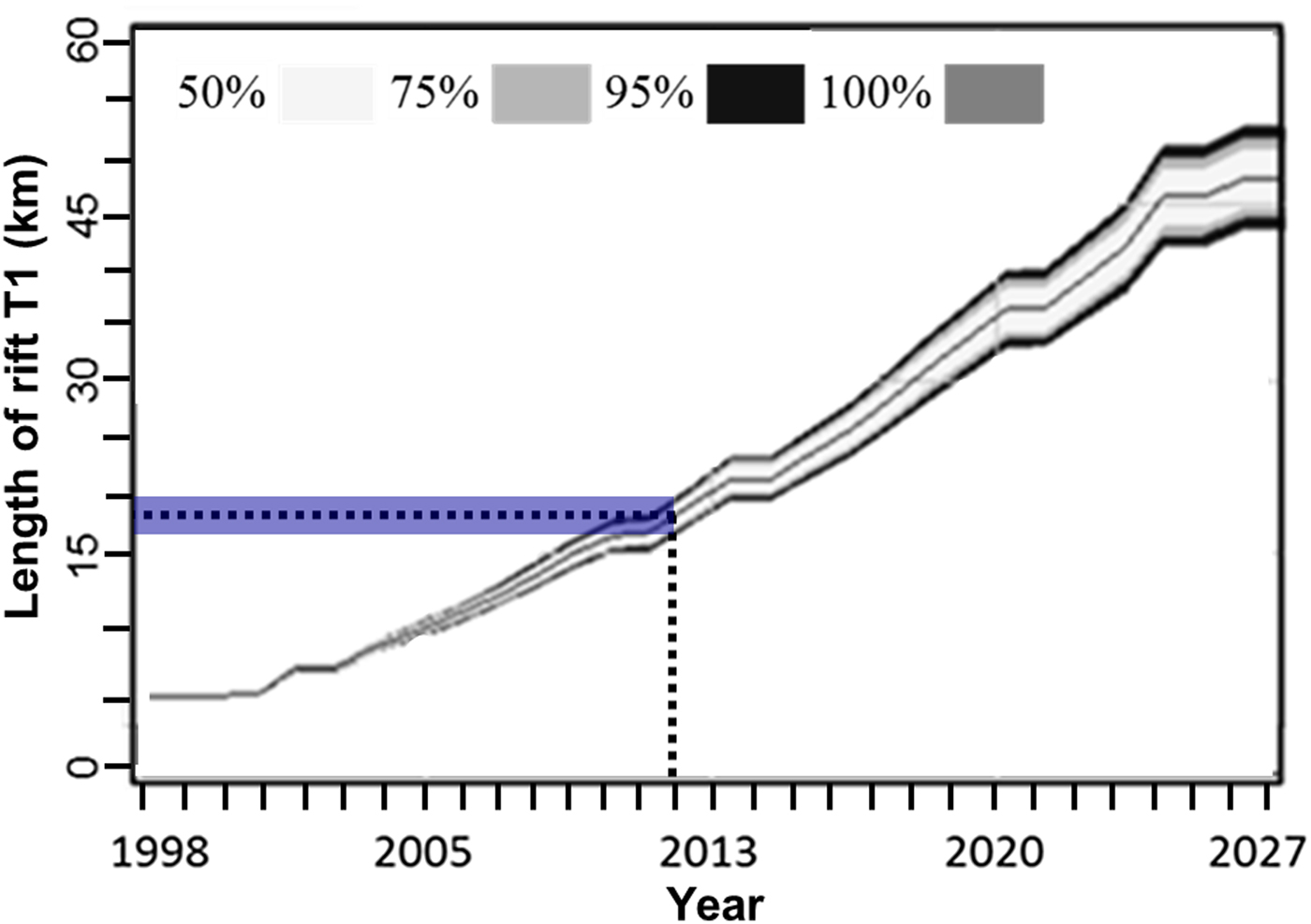
Fig. 8. Model validation using T1 as an independent sample. The length of T1 was measured to be ~20 km in late October 2011 (Fig. 4c), which places at the upper end of the simulated length of 18.5 ± 1.5 km (dotted lines, with blue hatched area indicating the ±1.5 km uncertainty in model predictions of T1 rift length). Coloured bands specify confidence levels as labelled.
Scenario testing
Scenario testing aims to (i) predict the most likely date at which the ‘Loose Tooth’ will detach; and (ii) identify which parameter in our predictor chain (Eqn 3) exerts the strongest control on it. We emphasize in this context that the level of any particular parameter in the predictor chain (Eqn (3)) reflects the strength of its correlation with all other parameters (Table 2), given our logical model (Fig. 3). This level must not be confused with the implied strength of control that the parameter exerts on RP and thus the prospective ‘Loose Tooth’ detachment date. We initiated our model runs using observed and extrapolated air temperatures in the same manner as during system validation. In addition to a ‘best-case’ standard model run we again conducted a large number of model sensitivity tests with data stream uncertainties and parameter variances of +/− 10%.
Predicted date of ‘Loose Tooth’ detachment
The detachment logic (Eqn 2) is central to the effort of detachment prediction in (i). Fricker and others (Reference Fricker, Young, Allison and Coleman2002) proposed that the Amery Ice Shelf has a major calving cycle of some 60–70 years, of which calving of large tabular icebergs from the ‘Loose Tooth’ embayment is part. While the next major calving event is not expected until the mid-2020s at the earliest, the ‘Loose Tooth’ was proposed to detach sometime between 2010 and 2015 (Fricker and others, Reference Fricker, Young, Allison and Coleman2002). Now, in late 2016, the ‘Loose Tooth’ has still not broken off and our system model allows us to make revised predictions of the detachment date. We predict respectively, at the 100 and 50% confidence levels that detachment will occur sometime between 2014 and 2025 and 2018 and 2021, with a predicted single-point date from the standard run in 2019 (Fig. 9).
Fig. 9. Simulated detachment dates of the ‘Loose Tooth’, using four different confidence levels, as indicated by grey shading. We predict respectively, at the 100 and 50% confidence levels that detachment will occur sometime between 2014 and 2025 and 2018 and 2021, with a predicted single-point date in 2019. Coloured bands specify confidence levels as labelled.
Parameter control of detachment date
Building our system architecture (see the section System Architecture) we discarded a range of parameters that did not show strong enough overall correlation with all other parameters (Table 3), given our logic model (Fig. 3). Discarded parameters included subsurface temperature (SST), air pressure (Pa), wind direction (WVD) and ice-shelf thickness (TH), while air temperature (T), relative humidity (RH), wind magnitude (WVM) and snow accumulation (AC) remained. To test which of the remaining parameters exerts the strongest control of the prospective ‘Loose Tooth’ detachment date, we compare the ‘best-case’ standard model run with sensitivity runs in which ±10% statistical variability of parameters are individually enabled (Fig. 10). The stronger the statistical control of any given parameter, the earlier the predicted detachment date will be.

Fig. 10. Parameter sensitivity to ‘Loose Tooth’ detachment date, for relative humidity (RH), wind magnitude (WM), accumulation (AC) and temperature (T). The standard run is as shown in Figure 9 (single point prediction date of 2019). For the sensitivity runs ±10% statistical variability of the labelled parameter is individually enabled (Fig. 10). The stronger the statistical control of any given parameter, the earlier the predicted detachment date. RH is thus identified as the best statistical predictor of ‘Loose Tooth’ calving, followed by WVM and AC/T.
The standard model run predicted a ‘Loose Tooth’ detachment data sometime in 2019, with an uncertainty of around 1 year (Figs 9 and 10). The 1-year uncertainty range also applies to the sensitivity runs, but in all cases resulted in earlier detachment dates than those in the standard run (Fig. 10). According to our sensitivity runs, relative humidity (RH) emerges as the strongest overall predictor with a ‘Loose Tooth’ detachment date sometime in 2014, followed by wind magnitude (WVM) and snow accumulation (AC) and air temperature (T) (both 2017, Fig. 10). In the case of air temperature (T) we must bear in mind that it was used to initiate the model and is therefore not an independently predicted parameter.
DISCUSSION AND CONCLUSIONS
Although Systems Analysis has previously been applied to glaciological problems, those applications were largely written from a technological perspective (e.g. Boyd, Reference Boyd2001). The main purpose of this paper was therefore to introduce Systems Analysis to a glaciological audience and provide an example of its application to iceberg calving as a topic of broad interest. Our study was motivated by the principles of statistical physics that are well suited to describing the large-scale and longer-term deterministic stochastic processes that control iceberg calving (Bassis, Reference Bassis2011). We demonstrated how the space-time behaviour of several environmental parameters might be captured in a system model, based on the common ‘V’-style Systems Analysis approach, of an ice shelf rift system that is trained with observations. Our study endorses Systems Analysis as a technique with promise in scrutinising iceberg calving as a complex glaciological process, and can motivate future work as follows.
Physical causality
Systems Analysis can evaluate the space-time behaviour of potential controls on an observed process, such as iceberg calving in the present case, from a statistical perspective. Although it cannot therefore evaluate physical causalities between parameters, it shows promise in identifying those parameters that are more likely to drive complex glaciological processes than others, and thus deserve further investigation. In the present case Fricker and others’ (Reference Fricker, Young, Allison and Coleman2002) ‘Loose Tooth’ detachment date of sometime between 2010 and 2015 turned out to be too early, and the application of Systems Analysis revises the date to ~2019 ±5 years. From our analysis relative humidity emerged as the strongest overall predictor of that date, followed by wind magnitude and snow accumulation. This assertion is puzzling because it is physically implausible that relative humidity can drive rift propagation, and the question arises as whether relative humidity measured at the G3 weather station is representative of the calving front.
The question can be answered by recalling that Systems Analysis does not imply physical causality; of the parameters considered here relative humidity measured at G3 is the best predictor of rift propagation, whether or not it is physically representative of the calving front. Simulations with the regional atmospheric climate model RACMO2 for the Lambert-Amery Ice Shelf system (e.g. Wen and others, Reference Wen2014) revealed that relative humidity is higher at the calving front compared with the inland location of G3, and similar trends are observed for surface albedo and solid precipitation (Fig. 11). Summer snowmelt is high everywhere on Amery Ice Shelf and thus maintains negative surface mass balance (SMB) in its inland areas, including the location of G3. Relatively elevated solid precipitation in contrast supports a positive SMB in the ice shelf's frontal portion (Fig. 11).

Fig. 11. Austral summer (DJF) averages of (a) relative humidity, (b) surface albedo and (c) snowmelt, as simulated with the regional atmospheric climate model RACMO2 for the Lambert-Amery Ice Shelf system.
Although a detailed physical analysis of cause and effect is beyond the scope of our study, the puzzle of physical plausibility can be addressed by considering relative humidity as a proxy for other parameters or processes that are capable of driving rift propagation. According to RACMO2 simulations (Van Wessem and others, Reference Van Wessem2014), relative humidity correlates best with surface albedo, and thus with net solar radiation. To a lesser extent, it correlates with snowmelt (Fig. 11), neither of which is included in our Systems Analysis. A lower albedo and lower relative humidity both emanate from increased föhn-driven surface melt, as observed on Larsen C Ice Shelf (Kuipers Munneke and others, Reference Kuipers Munneke, van den Broeke, King, Gray and Reijmer2012; Luckman and others, Reference Luckman2014). Higher RH may point to episodes with reduced föhn and katabatic flow, and perhaps increased advection of moist and precipitation from the coast, increasing albedo and inhibiting snowmelt. Snowmelt is intimately coupled to firn compaction and air depletion, and therefore the transport of heat into and the internal stress and flow fields of the ice shelf (Scambos and others, Reference Scambos2009; Holland and others, Reference Holland2011; Kuipers Munneke and others, Reference Kuipers Munneke, Ligtenberg, Van Den Broeke and Vaughan2014; Hubbard and others, Reference Hubbard2016). We can therefore postulate that changes in relative humidity can serve as a proxy for changes in the internal stress of the Amery Ice Shelf, which is a first order control of ‘Loose Tooth’ calving (Bassis and others, Reference Bassis, Fricker, Coleman and Minster2008). This postulate must be tested by future work.
4.2. Data limitations
For simplicity in demonstrating the utility of Systems Analysis in analysing complex glaciological processes, we used a coarse data set of weather station and visual observations of the ‘Loose Tooth’ on Amery Ice Shelf that may mimic many glaciological datasets from remote locations that are often sparsely sampled in space and/or time. In doing so we ignored other potential controls such as oceanographic conditions (Bassis and others, Reference Bassis, Fricker, Coleman and Minster2008; Depoorter and others, Reference Depoorter2013; Liu and others, Reference Liu2015) or mélange in rifts or suture zones (Bassis and others, Reference Bassis2007; Glasser and others, Reference Glasser2009; Hulbe and others, Reference Hulbe, LeDoux and Cruikshank2010; Jansen and others, Reference Jansen, Luckman, Kulessa, Holland and King2013; Kulessa and others, Reference Kulessa, Jansen, Luckman, King and Sammonds2014; McGrath and others, Reference McGrath2014), and our focus on yearly parameter averages did not allow us to examine seasonal and shorter-term changes in ‘Loose Tooth’ behaviour (Fricker and others, Reference Fricker, Young, Coleman, Bassis and Minster2005a, Reference Fricker, Bassis, Minster and MacAyealb; Bassis and others, Reference Bassis, Coleman, Fricker and Minster2005, Reference Bassis2007, Reference Bassis, Fricker, Coleman and Minster2008). Although as yet simplistic in glaciological terms, this initial application of System Analysis to tabular iceberg calving, as a typical complex glaciological process, can motivate follow-up work with datasets that are more finely sampled in space and time, and include a greater range of parameters.
ACKNOWLEDGEMENTS
We gratefully acknowledge support by Natural Environment Research Council (NERC) grants NE/L005409/1 and NE/E012914/1. We are grateful to the Australian Antarctic Division for online access to the Amery G3 Australian Antarctic AWS data, (http://aws.acecrc.org.au/datapage.html). We thank two anonymous referees for their helpful comments. RACMO2 model output was kindly prepared by J. M. van Wessem and M. R. van den Broeke, supported by funding from Netherlands Polar Programme and Netherlands Earth System Science Centre (NESSC).


 Open access