


1 INTRODUCTION
The Sloan Digital Sky Survey (SDSS) is one of the most widely used sky surveys. Also, it is the largest photometric and spectroscopic survey in optical wavelengths. Another widely used sky survey is the Two Micron All Sky Survey (2MASS; Skrutskie et al. Reference Skrutskie2006), which imaged the sky across infrared wavelengths. The third sky survey, which is an astrometrically and photometrically important survey, is Hipparcos (Perryman et al. Reference Perryman1997), re-reduced recently by van Leeuwen (Reference van Leeuwen2007).
SDSS obtains images almost simultaneously in five broadbands (u, g, r, i, and z) centred at 3 540, 4 760, 6 280, 7 690, and 9 250 Å, respectively (Fukugita et al. Reference Fukugita, Ichikawa, Gunn, Doi, Shimasaku and Schneider1996; Gunn et al. Reference Gunn1998; Hogg et al. Reference Hogg, Finkbeiner, Schlegel and Gunn2001; Smith et al. Reference Smith2002). The photometric pipeline (Lupton et al. Reference Lupton, Gunn, Ivezic, Knapp, Kent and Yasuda2001) detects the objects, matches the data from five filters, and measures instrumental fluxes, positions, and shape parameters. The magnitudes derived from fitting a point spread function (PSF) are accurate to about 2% in g, r, and i, and 3%–5% in u and z for bright sources (<20 mag). Data Release 5 (DR5) is almost 95% complete for point sources to (u, g, r, i, z) = (22, 22.2, 22.2, 21.3, 20.5) mag (we remind the reader about the recent data release of SDSS, DR6–DR9). The median FWHM of the PSFs is about 1.5 arcsec (Abazajian et al. Reference Abazajian2004). The data are saturated at about 14 mag in g, r, and i, and about 12 mag in u and z (see Chonis & Gaskell Reference Chonis and Gaskell2008).
The ugriz passbands on which the main SDSS with a 2.5-m telescope is based are very similar, but not quite identical, to the u′g′r′i′z′ passbands with which the standard Sloan photometric system was defined on the 1.0-m telescope of the USNO Flagstaff Station (Smith et al. Reference Smith2002). However, one can use the transformation equations in the literature to make necessary transformations between two systems (cf. Rider et al. Reference Rider, Tucker, Smith, Stoughton, Allam and Neilsen2004).
It has been customary to derive transformations between a newly defined photometric system and those that are more traditional, such as the Johnson–Cousins UBVRI system. The first transformations derived between the SDSS u′g′r′i′z′ system and the Johnson–Cousins photometric system were based on the observations in the u′, g′, r′, i′, and z′ filters (Smith et al. Reference Smith2002). An improved set of transformations between the observations obtained in the u′g′r′ filters at the Isaac Newton Telescope (INT) at La Palma, Spain, and Landolt (Reference Landolt1992) UBV standards is derived by Karaali, Bilir, & Tuncel (Reference Karaali, Bilir and Tuncel2005). The INT filters were designed to reproduce the SDSS system. Karaali et al. (Reference Karaali, Bilir and Tuncel2005) presented, for the first time, transformation equations depending on two colours.
Rodgers et al. (Reference Rodgers, Canterna, Smith, Pierce and Tucker2006) considered two-colour or quadratic forms in their transformation equations. Jordi, Grebel, & Ammon (Reference Jordi, Grebel and Ammon2006) used SDSS DR4 and BVRI photometry taken from different sources and derived population (and metallicity) dependent transformation equations between SDSS and BVRI systems. Chonis & Gaskell (Reference Chonis and Gaskell2008) used transformations from SDSS ugriz to UBVRI not depending on luminosity class or metallicity to determine CCD zero points. In Bilir et al. (Reference Bilir, Ak, Karaali, Cabrera-Lavers, Chonis and Gaskell2008), transformations between SDSS (and 2MASS) and BVRI photometric systems for dwarfs are given. Finally, we refer the recent paper of Yaz et al. (Reference Yaz, Bilir, Karaali, Ak, Coskunoglu and Cabrera-Lavers2010), where transformations between SDSS, 2MASS, and BVI photometric systems for late-type giants are presented.
Most of the transformations mentioned in the preceding paragraphs are devoted to dwarfs or the UV band has not been considered in the case of giants. We thought to derive transformation equations between either of the most widely used sky surveys, SDSS ugr, and UBV for giants. The saturation of the data in SDSS mentioned above restricts the range of the observed data in this system. Hence, we decided to use the synthetic ugr as well as UBV data. We used the procedure of Buser (Reference Buser1978), who derived two-colour equations between RGU and UBV photometries. The sections are organised as follows. Data are presented in 2. Section 3 is devoted to the transformation equations and their application and, finally, a summary and discussions are given in Section 4.
2 DATA
We used two sets of data. The U − B and B − V synthetic colours are taken from Buser and Kurucz (Reference Buser and Kurucz1992). Buser and Kurucz (Reference Buser and Kurucz1992) published the synthetic magnitudes and colours for 234 stars with different effective temperature, surface gravity, and metallicity. The ranges of these parameters are 3 750 ≤ Te ≤ 6 000 K, 0.75 ≤ log g ≤ 5.25 (cgs) and −3.00 ≤ [M/H] ≤ 0.50 dex. We combined the U − B and B − V colours for the surface gravities log g = 2.25 and 3.00 for the same temperature, and obtained a set of colours for the metallicities [M/H]= 0.00, −1.00, and −2.00 for six effective temperatures, i.e. 3 750, 4 000, 4 500, 5 000, 5 500, and 6 000 K for the red giants. This is the synthetic colour set in the UBV system of our sample used in the transformations.
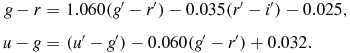
The u − g and g − r synthetic colours are provided from Lenz et al. (Reference Lenz, Newberg, Rosner, Richards and Stoughton1998). The authors synthesised the u′ − g′, g′ − r′, r′ − i′, and i′ − z′ colours with a large range of temperature, surface gravity, and metallicity using spectra from Kurucz (Reference Kurucz1991). The range of the temperature is rather large, 3 500 ≤ Te ≤ 40 000 K, for the colours with surface gravities corresponding to dwarfs or red giants, i.e. log g = 2.5, 3.0, 4.0, 4.5 (cgs) and metallicities [M/H]= 0.00, −1.00, −2.00 dex. However, a limited set of colours also exists for surface gravities log g = 1.0, 1.5, 2.0 (cgs) and metallicity [M/H]= −5.00 dex. We followed the procedure explained in the preceding paragraph and combined the u′ − g′, g′ − r′, and r′ − i′ colours for the surface gravities log g = 2.5 and 3.00 (cgs) for the same temperature, and obtained a set of colours for the metallicities [M/H]= 0.00, −1.00, and −2.00 dex for six effective temperatures, i.e. 3 750, 4 000, 4 500, 5 000, 5 500, and 6 000 K for the red giants. This is the synthetic colour set in the u′g′r′ system of our sample. As mentioned in Section 1, the main SDSS with a 2.5 m-telescope is based on instrumental ugriz passbands that are very similar, but not quite identical, to the u′g′r′i′z′ passbands with which the standard Sloan photometric system was defined on the 1.0-m telescope of the USNO Flagstaff Station (Smith et al. Reference Smith2002). Hence, we transformed the u′ − g′ and g′ − r′ colours of our sample to the u − g and g − r colours by the following equations derived by equations in Rider et al. (Reference Rider, Tucker, Smith, Stoughton, Allam and Neilsen2004):
 \begin{eqnarray}
g - r &=& 1.060(g^{\prime } - r^{\prime }) - 0.035 (r^{\prime } - i^{\prime }) - 0.025,\nonumber \\
u - g &=& (u^{\prime } - g^{\prime }) - 0.060(g^{\prime } - r^{\prime }) + 0.032.
\end{eqnarray}
\begin{eqnarray}
g - r &=& 1.060(g^{\prime } - r^{\prime }) - 0.035 (r^{\prime } - i^{\prime }) - 0.025,\nonumber \\
u - g &=& (u^{\prime } - g^{\prime }) - 0.060(g^{\prime } - r^{\prime }) + 0.032.
\end{eqnarray}
The data and the corresponding two-colour diagrams in the UBV and ugr systems are given in Table 1 and Figure 1.
Table 1. Synthetic colours as a function of effective temperature and metallicity.


Figure 1. The (U − B, B − V) and (u − g, g − r) two-colour diagrams for different metallicities: [M/H]= 0.00 (a and b), [M/H]= −1.00 (c and d), and [M/H]= −2.00 (e and f).
3 TRANSFORMATIONS
3.1 Transformation equations from UBV to ugr
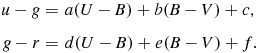
We adopted the following general equations to transform the U − B and B − V colours to the u − g and g − r colours for three sets of data with different metallicities given in Table 1, i.e. [M/H]= 0.00, −1.00, and −2.00 dex:
 \begin{eqnarray}
u - g &=& a ( U - B) + b ( B - V) + c,\nonumber \\
g - r &=& d ( U - B) + e ( B - V) + f.
\end{eqnarray}
\begin{eqnarray}
u - g &=& a ( U - B) + b ( B - V) + c,\nonumber \\
g - r &=& d ( U - B) + e ( B - V) + f.
\end{eqnarray}
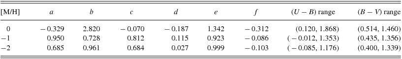
We used the least-squares method and evaluated the coefficients in Equation (2) for each set of data. The results are given in Table 2. The ranges of the (U − B) and (B − V) colours are also indicated in the last two columns of the table. The numerical values of the coefficients a and b for the metallicities [M/H]= −1.00 and −2.00 dex are close to each other, indicating that both colours are effective in the estimation of the u − g colour. However, for the metallicity [M/H]= 0.00 dex, the value of b is almost 9 times larger than the (absolute) value of a, which means that the B − V colour is much more effective than U − B in the estimation of the u − g colour, for solar metallicities. The case is different in the estimation of the g − r colour, i.e. the numerical value of e is at least 7 times larger than the numerical value of d for all metallicities. That is, the colour B − V plays a much more significant role relative to the colour U − B in the estimation of the colour g − r. The mean of the residuals for the u − g and g − r colours is almost zero, and the corresponding standard deviations are rather small, i.e. σ(g − r) ≤ 0.03 and σ(u − g) ≤ 0.09 mag.
Table 2. Numerical values for the coefficients in Equation (2) for three different metallicities. The U − B and B − V intervals in the last two columns indicate the ranges of these colours.
3.2 Inverse transformation equations
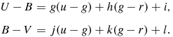
The general equations for the inverse transformations are adopted as follows:
 \begin{eqnarray}
U - B &=& g (u - g) + h (g - r) + i,\nonumber \\
B - V &=& j (u - g) + k (g - r) + l.
\end{eqnarray}
\begin{eqnarray}
U - B &=& g (u - g) + h (g - r) + i,\nonumber \\
B - V &=& j (u - g) + k (g - r) + l.
\end{eqnarray}
We applied the same procedure, i.e. the least-squares method, in the evaluation of the numerical values of the coefficients in Equation (3) for three different metallicities, [M/H]= 0.00, −1.00, and −2.00 dex, in Table 1. The results are given in Table 3. The ranges of the colours u − g and g − r are also indicated in the last two columns of the table. A comparison of the corresponding coefficients shows that g − r is effective in the estimation of U − B for metallicity [M/H]= 0.00 dex, while u − g is more effective in the estimation of the same colour for metallicity [M/H]= −2.00 dex. However, both g − r and u − g colours are equally effective for metallicity [M/H]= −1.00 dex. The case is different in the estimation of B − V, i.e. g − r is much more effective relative to the u − g colour. The means of the residuals for the U − B and B − V colours are almost zero and the standard deviations are small, i.e. σ(U − B) ≤ 0.06 and σ(B − V) ≤ 0.04 mag, except the standard deviation for the U − B colour for zero metallicity, i.e. σ(U − B) = 0.15 mag.
3.3 Application of the transformation equations
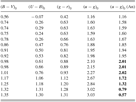
We applied the transformation equations to six clusters with different metallicities. The reason for preferring clusters instead of field stars is that they provide all the U − B, B − V, u − g, and g − r colours necessary for transformations. However, it is not easy to find a set of field stars with these colours and with different metallicities in the literature. The data for the clusters used in the application of the procedure are given in Table 4. The U − B and B − V colours are taken from the first reference, while the second reference (if it exists in the reference column) refers to the colour excess and metallicity.
Table 3. Numerical values for the coefficients in Equation (3) for three different metallicities. The u − g and g − r intervals in the last two columns indicate the ranges of these colours.
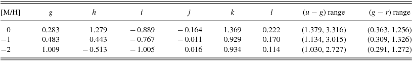
Table 4. Clusters used in the application of the procedure. The U − B and B − V colours are taken from the first reference, while the second reference (if it exists in the reference column) refers to the colour excess and metallicity.
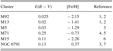
References. 1, Cathey (Reference Cathey1974); 2, Gratton et al. (Reference Gratton, Fusi Pecci, Carretta, Clementini, Corsi and Lattanzi1997); 3, von Braun et al. (Reference von Braun, Chiboucas, Minske, Salgado and Worthey1998); 4, Hodder et al. (Reference Hodder, Nemec, Richer and Fahlman1992); 5, An et al. (Reference An2008); 6, Fahlman, Richer & Vanderberg (Reference Fahlman, Richer and Vandenberg1985); 7, Sandage, Lubin & VandenBerg (Reference Sandage, Lubin and VandenBerg2003).
The transformation equations could be applied to the colours which fall into the ranges of the colours (U − B) and (B − V) stated in Table 2. The results are given in Table 5. The format of M13 is different from the other clusters, as explained in the following. For the evaluation of the (u − g)0 and (g − r)0 colours for the clusters M92, M15, M5, M71, and NGC 6791, we used the coefficients in Table 2 corresponding to metallicities close to the metallicities of these clusters, i.e. [M/H]=−2, −2, −1, −1, and 0 dex, while for the cluster M13, whose metallicity is in the middle of metallicity −1 and −2 dex, we used two sets of coefficients for each colour. One can notice small differences between the corresponding colours evaluated by means of two sets of coefficients.
Table 5. Transformation of the U − B and B − V colours to the u − g and g − r using the equations in (2).
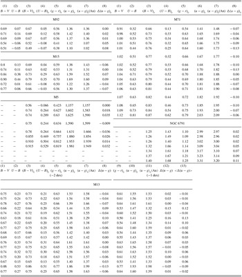
Columns (1) and (2): original (B − V) and (U − B) colours; columns (3) and (4): de-reddened (B − V)0 and (U − B)0 colours; columns (5) and (6): (g − r)0 and (u − g)0 colours estimated by the equations in (2); column (7): (u − g)0 colours evaluated by means of the calibrations of the fiducial sequences in An et al. (Reference An2008); and column (8): the residuals, Δ(u − g)0. The procedure has been applied twice for the data of M13, one for the metallicity [M/H]=−2 dex (columns 1–8) and one for [M/H]=−1 dex (columns 9–12). Column (13) refers to the mean of the residuals evaluated for two cases.
We evaluated the (u − g)0 colours using another procedure and compared them with those estimated by the transformation equations presented in this study, as explained in the following. We de-reddened the (u − g) and (g − r) colours in An et al. (Reference An2008) for the clusters in Table 4 and calibrated the (u − g)0 colours in terms of (g − r)0 ones for each cluster. Then, we applied these calibrations to the (g − r)0 colours transformed from the (U − B)0 and (B − V)0 colours. The (u − g)0 colours thus obtained are labelled as (u − g)0(An). The residuals, i.e. the differences between the (u − g)0 colours estimated by two different procedures, are given in the eighth column for the clusters M92, M15, M5, M71, and NGC 6791, while they are given in two columns, columns 8 and 12, for the cluster M13. Column 13 indicates the mean residuals (the other columns of Table 5 are explained under this table).
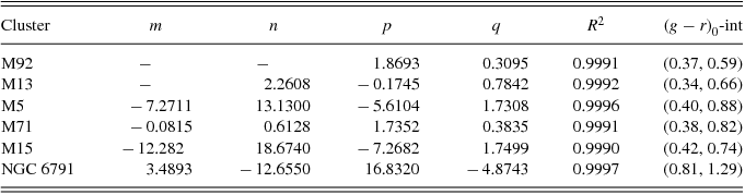
The calibration of (u − g)0 in terms of (g − r)0 for the fiducial sequences of the clusters in questions is adopted as follows:
 \begin{eqnarray}
(u - g)_{0} = m (g - r)_{0}^{3} + n( g - r)_{0}^{2}+ p(g - r)_{0} + q.
\end{eqnarray}
\begin{eqnarray}
(u - g)_{0} = m (g - r)_{0}^{3} + n( g - r)_{0}^{2}+ p(g - r)_{0} + q.
\end{eqnarray}
The numerical values of the coefficients are given in Table 6. The last column refers to the (g − r)0 range of the corresponding cluster. The (g − r)0 colours estimated by Equation (2), which are beyond the range of the corresponding cluster, could not be considered in our study and they are omitted from Table 5.
Table 6. Numerical values for the coefficients in Equation (4).
The mean and the corresponding standard deviation of the residuals are <Δ(u − g)0> = −0.01 and σ(u − g)0 = 0.07 mag, respectively, i.e. the (u − g)0 colour of a red giant would be estimated by the transformations presented in this study with an accuracy of Δ(u − g)0< 0.1 mag.
4 SUMMARY AND DISCUSSION
We presented metallicity-dependent transformation equations from UBV to ugr colours and their inverse transformations for red giants with synthetic colours. The ranges of the colours used for the transformations are rather large, i.e. 0.400 ≤ (B − V)0 ≤ 1.460, −0.085 ≤ (U − B)0 ≤ 1.868, 0.291 ≤ (g − r)0 ≤ 1.326, and 1.030 ≤ (u − g)0 ≤ 3.316 mag, and cover almost all the observational colours of red giants. However, one cannot obtain a set of observed colours with a large range and with different metallicities available for transformations. We derived three sets of transformations for metallicities [M/H]= 0, −1, and −2 dex. The researcher can use the transformation coefficients in Table 2 (or Table 3 for inverse transformations) regarding the metallicity of the red giant in question. One can also use two transformation equations and make an interpolation between two sets of results according to the metallicity of the star, similar to our calculations for the red giants in the cluster M13 (Section 3.3).
We applied the procedure to two clusters of different metallicities as two examples, i.e. we derived the (g − r)0 and (u − g)0 two-colour diagrams for M5 (Table 7) and NGC 6791 (Table 8) by the transformation of the (U − B)0 and (B − V)0 colours of these clusters and plotted them in Figures 2 and 3, respectively. The points corresponding to the data evaluated via the red giant sequences in An et al. (Reference An2008), i.e. 0.4 ≤ (g − r 0 ≤ 0.82 and 1.16 ≤ (u − g)0 ≤ 1.98 mag for M5, and 1.09 ≤ (g − r)0 ≤ 1.25 and 2.98 ≤ (u − g)0 ≤ 3.31 mag for NGC 6791 overlap the diagrams, confirming our argument.
Table 7. The (u − g)0 − (g − r)0 two-colour red giant sequence of M5 derived from the (U − B)0 and (B − V)0 colours of the same cluster.
The last column refers to the (u − g)0 colours evaluated by means of the red giant sequence in An et al. (Reference An2008). The figures in boldface correspond to the (g − r)0 colours which lie beyond the range of the cluster and which are not considered.
Table 8. The (u − g)0 − (g − r)0 two-colour red giant sequence of NGC 6791 derived from the (U − B)0 and (B − V)0 colours of the same cluster (the explanation of the columns is the same as in Table 7).
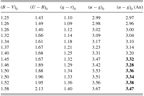
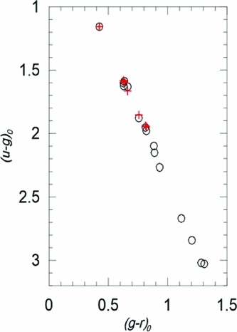
Figure 2. The (u − g)0 − (g − r)0 two-colour diagram of M5 based on the transformations in this study (○). The points corresponding to the data evaluated via the red giant sequence in An et al. (Reference An2008) are also plotted in this diagram (+).

Figure 3. The (u − g)0 − (g − r)0 two-colour diagram of NGC 6791 based on transformations in this study (symbols as in Figure 2).
Also, we plotted the observed Johnson colours versus observed and predicted SDSS colours for the clusters M5 and NGC 6791 to see the trends of two sets of data. We illustrated the data for M5 in Figure 4 in two panels. Figure 4(a) gives the variations of the observed (u − g)0 data (symbol: +) and the predicted ones (symbol: ○) relative to the observed Johnson colour (U − B)0, while those for the (g − r)0 colour relative to (B − V)0 are shown in Figure 4(b) with similar symbols. The data for NGC 6791 are plotted in Figures 5(a and b), similar to Figure 4. We should note that the observed (g − r)0 and (u − g)0 colours are restricted with their ranges, as stated in the foregoing paragraph.

Figure 4. Observed Johnson colours versus observed (+) and predicted (○) SDSS colours for the cluster M5: (a) (U − B)0 versus (u − g)0 and (b) (B − V)0 versus (g − r)0.

Figure 5. Observed Johnson colours versus observed (+) and predicted (○) SDSS colours for the cluster NGC 6791: (a) (U − B)0 versus (u − g)0 and (b) (B − V)0 versus (g − r)0.
The mean and the standard deviation of the residuals for each cluster as well as for their combination are given in Table 9. The ranges of the mean and the standard deviation of the residuals for all clusters are −0.08 ≤ <Δ(u − g)0> ≤ 0.05 and 0.02 ≤ σ(u − g)0 ≤ 0.07 mag, respectively. While their mean and standard deviation are <Δ(u − g)0> = −0.01 and σ(u − g)0 = 0.07 mag, respectively. That is, the (u − g)0 colours would be estimated by our transformations with an accuracy of Δ(u − g)0 ≤ 0.08 mag.
Table 9. The mean and standard deviation of the residuals for each cluster and for their combination.
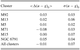
The probable parameter which would affect the colours estimated by the transformations in this study is the interstellar reddening. We confirmed our argument by applying the transformations to the data of the cluster M71 for two-colour excesses, i.e. E(B − V) = 0.25 and 0.32 mag, which are taken from An et al. (Reference An2008). The corresponding standard deviations are equal, σ(u − g)0 = 0.034 mag, whereas the means of the residuals are different, i.e. <Δ(u − g)0> = −0.078 and −0.103 mag, for the colour excesses E(B − V) = 0.25 and 0.32 mag, respectively. We adopted the colour excess E(B − V) = 0.25 mag in our statistics.
The transformation equations presented in this study can be applied to clusters as well as to field stars. It will be rather fruitful to derive the (u − g)0 − (g − r)0 fiducial sequences of the red giants for some clusters whose metallicities are compatible with the metallicities of some populations. The cluster 47 Tuc can be given as an example for the Intermediate Population II or thick disc. One can use the colour magnitude diagram of this cluster to evaluate the Mg absolute magnitudes of the red giants of the thick disc population and estimate Galactic model parameters for this population.
ACKNOWLEDGEMENT
We thank an anonymous referee for comments and suggestions.


