


Introduction
In recent years, advancements in computing power and analytical algorithms have led to significant developments in scientific research [Reference Fortunato1,Reference Eliceiri2]. Microscopy and analytical imaging have greatly benefited from these innovative approaches, leading to breakthroughs pertaining to cellular, molecular, and genomic biology [Reference Eliceiri2–Reference Pegoraro and Misteli5]. There are several different terms used when referring to modern analytical imaging approaches of biological systems. High content screening (HCS) is a term often used to describe the use of an automated imaging system and large data sets to screen drugs or other biological analytes and to assess their endpoint effects on cellular populations [Reference Zock6,Reference Buchser and Markossian7]. For smaller data sets (often less than 100,000 data points), the preferred terminology is high content imaging (HCI) [Reference Buchser and Markossian7]. High content analysis (HCA) is used to describe automated analytical software used to process images or data acquired via HCS or HCI [Reference Buchser and Markossian7]. Depending on the system or application of interest, HCA systems can autonomously quantify pre-defined biological endpoints of interest that include fixed samples, cell suspensions, cell cultures, microplates, or histopathological biopsies [Reference Roukos and Misteli3,Reference Pegoraro and Misteli5]. These new and evolving microscopy techniques have become widespread and are being integrated into research as a key aspect of data acquisition and analysis [Reference Zock6,Reference Buchser and Markossian7]. Additionally, due to the ability to process large amounts of data rapidly, HCA techniques are growing in popularity in diagnostic and clinical institutions, such as hospitals and pharmaceutical companies [Reference Gurcan8–Reference Abraham10].
HCA allows analysis of samples with minimal or no user intervention, while still allowing for additional manual analysis if necessary [Reference Zock6,Reference Buchser and Markossian7]. Standardizing the analytical process with automated HCA-based methods improves robustness, validity, and reproducibility of sample analysis while minimizing observer bias [Reference Gurcan8,Reference King and Long11]. Additionally, this frees up time for researchers or clinicians to process more samples and collect data in less time than standard manual observation and analysis [Reference Buchser and Markossian7].
The development of real-time HCA-based approaches to analyze diagnostic and histopathological tissue samples, such as biopsies for cancer, autoimmune diseases, and traumatic or chronic wounds, could significantly improve patient care [Reference Roukos and Misteli3,Reference Pegoraro and Misteli5]. Analytical imaging is extremely important when considering a pathologist's role in evaluating tissue samples to assist clinicians in potential patient diagnoses [Reference Aeffner12]. Frequently, in a clinical setting, a biopsy specimen is benign and has common simple characteristics or patterns that can easily be analyzed [Reference Gurcan8]. Therefore, pathologists often spend more time sifting through benign specimens rather than focusing on samples with complex pathologies that require more intensive analysis [Reference Gurcan8]. Currently, there is need for effective and economical approaches to analyze samples to relieve this time burden for pathologists and researchers. Moreover, repetitive measurement tasks are especially at risk for reliable and reproducible analysis of samples. This is due to inherent variability between the same and different individuals that perform the analysis over time (intra- and inter-rater reliability) [Reference Hallgren13–Reference Lee15].
The burden of labor-intensive manual analysis and the potential for inter- and intra-rater variability highlights the importance of developing automated quantitative image analysis methodologies. Although all data collected must be taken into context of sample collection, processing, and imaging, the overall HCA process streamlines analytical imaging and provides a more quantitative assessment. Currently, many HCA approaches utilize commercial-based systems that are only compatible with proprietary HCI or HCS imaging systems. These setups can be a large financial commitment, making it difficult for researchers that only perform occasional analysis of large data sets to benefit from such an approach. This is less of a problem for core imaging facilities, but these core facilities often have an overburdened staff.
Providing accurate high-throughput analytics will allow clinicians, pathologists, and researchers to standardize quantification of discrete attributes of samples, such as assessing an inflammatory infiltrate by calculating cell numbers or measuring tissue thickness to determine the level of fibrosis of a wound. These are characteristics that offer significant amounts of information about the status of a tissue and provide assessment of potential prognostic features. Approaches that can efficiently analyze large tissue specimens with minimal user intervention, when compared to traditional analyses for predefined macro- and micro-cell characteristics, will make tissue analytics more reliable and economical. For example, analysis of wound healing in skin is often hindered when associated with sustained levels of inflammation [Reference Guo and DiPietro16]. Therefore, an HCA-based approach could allow pathologists to assess the status of different layers of a superficial wound, such as a diabetic ulcer, as it heals [Reference Wang17]. Throughout the healing process the layers of skin (keratin, epidermis, dermis, and subcutaneous) tend to fluctuate in thickness due to fibrosis, migration of cells, and infiltration of edematous fluid [Reference Blair18,Reference Xue and Jackson19].
The clinical benefit of an effective HCA-based approach could help define future treatment for patients with chronic or traumatic wounds. HCA will improve the reproducibility and statistical rigor of data regarding biological specimens from both in vitro and in vivo studies while enabling processing of multiple samples simultaneously [Reference Horvath20,Reference Bray, Carpenter and Markossian21]. For instance, the size or density of an inflammatory infiltrate within a wound could be more precisely defined and compared across multiple samples. Therefore, there is a need for a cost-effective HCA-based approach, compatible across multiple imaging platforms, that can analyze an image of an entire large tissue specimen. Additionally, it would be advantageous for this method to be able to preserve high-resolution characteristics of cell-based features after digital magnification without reimaging at different magnifications to analyze specific features, while also remaining compatible with a variety of staining methods to provide a holistic perspective of the sample.
In this study, we present a customized method for a HCI automated approach that uses iterative machine-assisted capture of multiple high-resolution images of a single tissue section, which are then stitched together to form a single high-resolution image. This method permits the user to program image analysis software to create regions of interest (ROIs) that maintain the curved contours typically found in biological specimens. Discrete image features based on parameters such as size and shape can be analyzed. Moreover, the use of histological staining can further maximize the specificity of image analysis by providing an additional layer of image differentiation based on color intensity. This automated approach allows analysis of macrostructures from the reconstructed image for analysis of features such as the morphology and thickness of skin layers within a wound. Additionally, the method provides the capability to evaluate critical microstructures such as individual nuclei within a cell or tissue from the reconstructed image without loss of resolution. This approach can be used with sections from virtually any type of tissue imaged using a wide array of methods.
Methods
Animal use, surgery, and tissue harvest
Experiments were approved by the University of Kansas Medical Center (KUMC) Institutional Animal Care and Use Committee (IACUC #2016-2319). Hodge et al. previously described animal handling, surgical, and tissue harvesting methods [Reference Hodge22]. Two female 4-month-old miniature Yucatan pigs (Auxvasse, MO) were acclimated for 14 days in an AAALAC-accredited facility with ad libitum access to food and water. Under general anesthesia, a custom biopsy punch was used in conjunction with a 3D-printed acrylonitrile butadiene styrene (ABS) guide to create a series of 1cm3 wounds on both the left and right sides of the animal's back (8 per side, 16 total). Harvested biopsies were roughly bisected. One half of the excised tissue block was preserved in 10% neutral buffered formalin (NBF), and the other half was preserved in RNAlater® (Sigma-Aldrich, St. Louis, MO).
Histological processing
Tissue placed in 10% NBF was fixed for a minimum of one week prior to being washed with phosphate buffered saline (PBS) and placed in 70% ethanol for a minimum of 24 hours. Samples were sent to Charles River Laboratories (Wilmington, MA) for serial sectioning (10 μm thickness) and staining using in-house protocols. Every third serial section was stained in a repeating pattern of hematoxylin and eosin (H&E), Masson's Trichrome (MT), and Brown and Brenn (BB).
Image acquisition and reconstruction
The end goal of the image acquisition and reconstruction process was to generate a composite image of the entire tissue section suitable for gross tissue measurements while providing sufficient resolution to facilitate segmented, cell feature-based automated quantification. This allows for both gross histological measurements and fine cell feature quantification using the same image set.
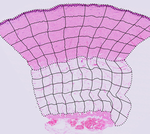
A Nikon Eclipse Ti-automated imaging system equipped with a Nikon DS-Fi3 camera and NIS-Elements HCA imaging software (Nikon Instruments Inc., Melville, NY) was used to acquire full-color, 8-bit, RGB images for the entirety of each tissue section at 200× total magnification. Images were saved as *.ND2 files. Approximately 375 and 650 individual images were acquired for the two tissue sections used in this paper. The complete image sets were precisely stitched together based on the (x, y) coordinates of each individual image using NIS-Elements software, resulting in reconstruction of the complete tissue section (Figures 1A, 1B). The reconstructed images were 6.5 GB and 11.5 GB, although file sizes can easily reach >30 GB as dimensions of the tissue section increase. File sizes >4 GB restricted the available file formats in which the images could be saved; reconstructed sections were saved as LIM ND2 files. This imaging and reconstruction approach resulted in an image resolution of 0.17 μm/px.

Figure 1: ROI boundary creation and image segmentation. (A, B) Reconstructed tissue sections from 200× total magnification images where (A) is control tissue and (B) is injured tissue after 9 days of recovery. These two tissue sections are overlaid with black, dotted lines indicating the tissue layer boundaries. These dotted lines are used to create the completed ROI grid. (C, D) The ROI column and row blends (black, solid lines) overlaid with the dotted line tissue layer boundaries create the complete set of ROI boundaries. (A–D) Modified images from Hodge et al. [22].
ROI boundary creation and image segmentation
The image analysis approach in this paper subdivides each section into multiple, distinct ROIs as a function of tissue layer. Furthermore, ROI creation seeks to accurately capture and maintain the irregular contours of the tissue while excluding negative space outside the tissue boundaries. Adobe Illustrator (Adobe, San Jose, CA) was used for ROI boundary creation because of its precision controls for vector-based linework, which was then used in NIS-Elements.
To create the ROIs for a reconstructed section, the ND2 files were opened in NIS-Elements and scaled down for export as TIFF files (4 GB maximum file size). The relative percent size reduction of the TIFF was recorded for future reference. The TIFF file was opened in Adobe Illustrator, centered on the artboard of equal size, and locked. On a separate layer, the upper contour of the keratin, epidermal and dermal layers, and the upper and lower contours of the subcutaneous layer were traced using the Pen tool. Similarly, the right and left contours of the tissue section were traced on their own layer, and then cut using the Scissors tool to create layer-specific boundaries. In aggregate, these contours collectively defined the upper, lower, left, and right boundaries of each tissue layer (Figures 1A, 1B). The adjacent tissue sections, stained with MT and BB, were used as visual references, when needed, to best determine where the tissue layer boundaries should be placed.
Using the Blend tool, the leftmost control points on the upper and lower boundaries of the dermis were selected and the blend parameters were set to create a horizontal midline (Object > Blend > Blend Options… > Spacing > Specified Steps = 1). Similarly, using the Blend tool, the topmost control points of the left and right tissue layer contours were selected, and the Blend parameters were set to create a smooth transition across 10 “columns” or divisions of approximately equal width midline (Object > Blend > Blend Options… > Spacing > Specified Steps = 9). The blend containing the column divisions and the dermis midline were both selected, and the Blend spline was replaced with the midline (Object > Blend > Replace Spline) so the column divisions more closely approximated the general curvature of the tissue section. The same general process was repeated to create 10 columns for the subcutaneous layer. Using the Blend tool, the leftmost control points for the upper and lower boundaries of the dermis were selected, and the Blend parameters were set to create a smooth transition across 5 “rows” or divisions of approximately equal height for both the dermis and subcutaneous layers. The column and row grids were overlaid on the tissue layer boundaries to create the completed ROI grid for the tissue section (Figures 1C, 1D). The image of the tissue layer was hidden leaving only the black lines of the ROI grid visible, and the grid was exported as a TIFF file.
In NIS-Elements, the ROI grid and ND2 file for the paired full-size tissue section were both opened, and the ROI grid was scaled up to match the document size of the tissue section. The ROI editor was opened in the file containing the ROI grid, and the auto-detect tool was used to identify the regions. The ROI set was saved and then loaded in the file containing the stained tissue section.
Tissue thickness measurements
Thickness of the tissue layers can vary considerably across the width of the sample, particularly in wounded tissue, which makes single-point sampling of a given layer inaccurate. To offset this variability, a maximum of 10 thickness measurements per layer per tissue section were collected (Figure 2). These 10 measures correspond to one thickness measurement per column, which pairs efficiently with the previously established ROI grid. Distance measurements could also be applied to other specific ROIs or wound features if desired. Layer thickness measurements were not collected using automated processes. For each column of ROIs in a tissue layer, the midpoints of the topmost ROI and the bottommost ROI were connected, and a straight line connecting the ends of the midpoints was measured and recorded.

Figure 2: Tissue layer thickness measures. (A, F) Reconstructed tissue sections from 200× total magnification images with colored, dashed lines indicating where measurements took place wherein (A) is control tissue and (F) is injured tissue after 9 days of recovery. The color and location of each linear measurement indicated on the figure correspond to the same color-coding of the scatterplots; however, due to the size of the image and the relative thinness of the keratin and epidermis tissue layers, a single magenta line was used to represent the separate thickness measure for both layers. The thickness of each tissue layer for control and injured tissue sections are shown in scatterplots: keratin (B, G; black open circles), epidermis (C, H; magenta open squares), dermis (D, I; turquoise open triangles), and subcutaneous (E, J; purple open diamonds). In the injured tissue, not all layers were present at all sample locations, and the keratin layer and epidermis have only 5 of 10 possible measurements, although the dermis and subcutaneous layers do have all 10 measurements. (A, F) Image sets used to provide visual context. Images from Hodge et al. [22].
Automated cell feature counting
The previously reconstructed images of H&E-stained tissue that were overlaid with the ROI grid were scaled down in size to prevent the software from crashing during analysis. Resolution of the images used for analysis was 0.51 μm/px. A custom, automated image analysis scheme was developed in NIS-Elements software that allowed the number of nuclei in all ROIs for each tissue layer to be quantified. Although all images were acquired using brightfield microscopy, individual RGB channel color data were used extensively during the analysis process to better filter or identify cell nuclei, since each channel had different degrees of color contrast between specific cell features. Analysis parameters were designed to be specific for each tissue layer due to the distinct staining patterns as follows:
• Keratin layer images were analyzed using the green channel from the full-color images. Images were pre-processed using auto contrast and soothing commands prior to being subjected to an over/under threshold that was further refined by filling holes, eroding, and filtering based on width.
• Epidermal layer images were analyzed using data from the red and green channels, and nuclei were identified by having specific positive characteristics in both channels. In the red channel, images were pre-processed using local contrast and soothing commands prior to being subjected to a dark spot detection threshold with settings for diameter and contrast. This was further refined using a thickening command. In the green channel, images were subject to smoothing and auto-contrast commands prior to being subjected to an over/under threshold that was refined using dilated and filter-on-area commands.
• Dermal layer images were analyzed using data from red, green, and blue channels. Nuclei were identified by having specific positive characteristics in the red and green channels while having specific negative characteristics in the blue channel. In the blue channel, images were pre-processed using a detect peaks command and then subjected to an over/under threshold that was refined by dilating and eroding the threshold binary to close minor holes, and then filtered based on circularity. In the green channel, images were not pre-processed but were subjected to a dark spot detection threshold with settings for diameter and contrast. This was further refined using erode and filter-on-area commands. In the red channel, images were pre-processed using auto contrast and soothing commands, prior to being subjected to an over/under threshold that was further refined by filling holes, eroding, and filtering based on elongation.
• Subcutaneous layer images were analyzed using data from the red channel. Images were not pre-processed but were subjected to a dark spot detection threshold with settings for diameter and contrast, which was further refined using erode and filter based on elongation commands.
Using the parameters described above, the macro was run to quantify cell nuclei per ROI in addition to calculating the area of each ROI.
Results
Tissue layer thickness measurements
In Figure 2, the thickness of the keratin (Figures 2B, 2G), epidermis (Figures 2C, 2H), dermis (Figures 2D, 2I) and subcutaneous (Figures 2E, 2J) layers are displayed in the control and wounded tissues. Non-injured tissue displayed less variation in thickness across each tissue layer than injured. In the injured tissue, not all layers were present at all sample locations, and as a result the keratin layer and epidermis thickness measurements have 5 data points out of the possible maximum of 10. This did not impact measurement acquisition. Variation in thickness data points is inherent to the intrinsic variability of layer thickness (especially wounded sample) across the tissue specimen, not as a result of the methodology. Additional histological stains are seen in Figure 3 to demonstrate the capacity to utilize the thickness quantification across multiple staining modalities. Supplementary stains, such as MT (Figures 3A, 3B) can be used to aid in the identification of tissue layers and/or regions based on collagen (blue) and keratin (red) staining, whereas BB (Figures 3C, 3D) helps identify regions populated by gram positive (purple) and gram negative (red/pink) bacteria.

Figure 3: ROI boundary creation and image segmentation of MT and BB. (A–D) Reconstructed tissue sections from 200× total magnification images: (A, C) control tissue and (B, D) injured tissue after 9 days of recovery. Images are overlaid with black, dotted lines indicating the tissue layer boundaries. These dotted lines were used to create the completed ROI grid. The ROI column and row blends (black, solid lines) overlaid with the dotted line tissue layer boundaries create the complete set of ROI boundaries for (A, B) MT and (C, D) BB stained samples. (A–D) Modified images from Hodge et al. [22].
ROI area, nuclei counts, and density
Data output from the macro included the number and area of the counted objects, area of the ROI, and the area fraction of the counted objects within the ROI. Several other parameters can added to the data output in an experiment-specific fashion. Descriptive statistics for the ROIs are shown in Tables 1 and 2 for control and injured tissue, respectively. The number of counted objects and ROI area were used to calculate the density of the counted objects for each ROI.
Table 1: ROI descriptive statistics: control tissue.

Table 2: ROI descriptive stats: wounded tissue.

In Figure 4, results of the automated nuclei quantification are displayed as densities to control for variation in ROI size. ROIs for both injured and control tissue cell densities followed the same general trends. Cell densities from lowest to highest were found in the keratin, subcutaneous, epidermis, and dermis tissue layers, although the average density and spread of cell densities for control and injured tissue differed. The average density ± standard error of the means (S.E.M.) are reported in Table 3 for both control and injured tissues. Table 4 gives examples of many of the commands used in the macro for nuclei counting, along with example settings and very broad potential uses. Table 4 further elaborates on the “positive” and “negative” characteristics used in this methodology. The exact settings are dependent on the operator and staining modality/intensity and, thus, Table 4 provides generalized parameters that can be used to perform quantification of objects such as cell nuclei.

Figure 4: Quantification of nuclear density as a function of ROI. (A–H) Scatterplots displaying the density of quantified nuclei/10,000 μm2 for all ROIs in each of the 4 tissue layers: keratin, epidermis, dermis, and subcutaneous layers, respectively for control (A–D) and injured (E–H) tissue. Quantified nuclei are represented in the images by blue dots. (I–N) Representative images highlighting the tissue layers in control and injured tissue. (I, L) Showing the relatively low nuclear density observed in the keratin layer and the typical density in the epidermis. (J, M) Contrasting the stark difference in the density of the dermis in control versus injured tissue. (K, N) Displaying the density ROIs for the subcutaneous layer.
Table 3: Average cell density in ROIs.

Table 4: Example of macro commands for subject identification.

Discussion
HCA is part of a growing field of analytical imaging that uses fully or semi-automated systems to assess image features. Imaging software provides an approach to quantitative analytical imaging that has the potential to benefit both researchers and clinicians. With the capabilities of high-resolution imaging growing, it is important to develop methods that are accessible and provide quantifiable data from the dense amount of information provided by imaging and histopathological analysis techniques. We present a potential combination of methods for improving ways users can extrapolate information from tissue specimens and decrease the inherent bias of current manual approaches in the study of diseases.
One of the many benefits of this methodology is that it can be used with essentially any image. This includes macroscopic tissue images down to electron microscopy images, and everything in between. After multiple high-resolution images are acquired, a single image is developed by reconstructing the individual images via stitching. The user can then determine specific image features of interest for analysis. Once the image feature is determined, customizable ROIs of any shape and size can be created. If the target of interest is a micro-level feature like nuclei, as performed in this study, then automated counting can be applied based on the color, shape, or size of the image feature.
Differentiation of image features based on color is maximized by utilizing staining or labeling methods to enhance features and to remove background noise. Additionally, shape and size for image feature differentiation can be used to further qualify components of the image and increase the specificity of feature quantification. A unique feature of this method is its ability to work effectively with non-uniform shapes and tissue samples, which can often provide problems for other HCA systems that rely on rigid gridding and geometrical shapes.
As shown in this study, one can count nuclei, but if specific cell populations are of interest, then a different stain or counterstain can be applied to enhance specificity of the nuclear quantification. The ability to use this methodology with multiple staining/labeling techniques, or even without staining/labeling, allows for customization of a variety of image features. If a macro-level feature is of interest, such as tissue thickness or quantification of tumor size, then an automated ROI approach or manual analysis of the tissue can be performed.
Sometimes manual analysis of certain image features is ideal. This method enhances the ability of users to perform manual analysis of image features by going from low optical to higher digital magnification with the same image, where image resolution is only limited by the processing power of the computers used for analysis.
Moreover, this method can be used to validate accuracy and reliability of manual measurements of image features to assess inter- and intra-rater reliability. It is important to recognize that there are many inherent biases during image analysis. Biases can be dependent on tissue collection, processing, mounting, staining, imaging software, or user. Therefore, a more autonomous approach to the processing and analysis of images can help prevent bias and improve the rigor of the data collected.
This method can also work in tandem with machine-based learning programs to enhance a data set or to validate the accuracy and reproducibility of machine-based learning programs, such as CellProfiler™. The discrete data generated by characterizing the custom ROIs (Tables 1–3) can aid in construction of machine-based learning programs. One important difference between our method and a machine-based learning program is that the exact qualifying parameters utilized and how they are being generated is known. In machine-based learning there is less awareness of the dynamic algorithms being used to quantify image features. For certain applications, machine-based learning programs are likely more efficient, such as more in-depth analysis of complex systems. However, reproducibility of machine-based learning programs can often be subjective and contain inherent biases from the operator.
Lastly, the method in this study provides a financial advantage. As previously stated, this approach can be paired with almost any imaging system or analysis software that a laboratory may currently have without the need to purchase new equipment or software. Therefore, the financial burden that plagues many HCA systems, that may come as part of compatible HCI or HCS systems, can be bypassed to permit greater access to the wealth of data provided by image analytics. The measurement of tissue layer thickness was limited only by the presence/absence of tissue layers in the images. The quantification of nuclear density, as a function of ROI, was mildly limited by stability of the analysis software when handling large file sizes and the processing power of the computer.
In summary, this methods study demonstrated a new analytical imaging technique that involves a combination of HCI and the reconstruction of images to generate a single high-resolution image. This newly generated image can be customized by segmenting the image into ROIs. Notably, this method works well with non-uniform and organic contours of biological specimens, such as that from a clinical biopsy, which is often problematic for other HCA methods that rely on rigid geometry methods. A wound healing model was used to demonstrate some of the common features of this method. Nuclei counts and tissue thickness measurements were chosen to demonstrate the micro- and macro-capabilities of this method. Additionally, we discuss how the automated features limit the inherent biases and errors that often plague quantification of image features, especially those that require repetitive analysis. Moreover, the method can be used across various platforms in tandem with other HCA methods, including machine-based learning, to improve data rigor and reproducibility. Ultimately, this method can aid both clinical and academic researchers by providing a more economical approach to image analysis.


