


Impact Statement
The evolution of sediment plumes is a multiscale and multiphysics process of great complexity that plays a key role in setting the indirect impact of deep-sea mining activities. Most recent efforts to model such plumes have relied on large-scale numerical simulations of specific operational parameters over time scales that are much smaller than the typical duration of an operation. As a result, considerable uncertainty remains as to the role played by key physical oceanography and operational parameters on setting the extent of plumes. In addition, the very definition of the extent metric of interest plays a foundational role in setting the impact of plumes. The work presented herein takes a more fundamental simplified approach that aims at gaining a first order understanding of the extent of sediment plumes over long time scales, and how it varies with the key parameters. The findings can guide future efforts to characterize impact and inform future research.
1. Introduction
In several regions of the world's oceans, extended portions of the seabed are bestrewn with polymetallic nodules that contain metals of interest to society (Reference Peacock and AlfordPeacock & Alford, 2018). Emerging technologies being designed to gather these nodules comprise collector vehicles that pick up the nodules, a commonly proposed pick up mechanism being hydrodynamic suction, and a vertical transport system that brings the nodules up to a surface operation vessel (Reference SharmaSharma, 2017); see figure 1. In gathering the nodules, the collector vehicle will also pick up several centimetres of the top layer of sediment of the seabed. The majority of this resuspended sediment will be separated from the nodules inside the collector vehicle and discharged in its wake, producing a so-called collector plume. A fraction of the resuspended sediment will be taken up to the surface operation vessel by the vertical transport system along with the nodules, where it will be separated from the nodules, and potentially subsequently discharged at depth, producing a so-called midwater plume (Reference Oebius, Becker, Rolinski and JankowskiOebius, Becker, Rolinski, & Jankowski, 2001).

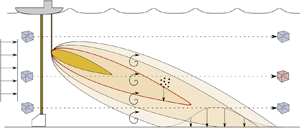
Figure 1. Sketch of a steady-state plume resulting from a midwater discharge of sediment during deep-sea nodule mining operations (not to scale). A uniform background flow is used to illustrate how advection transports sediment away from the point of neutral buoyancy reached by the plume following the buoyancy-driven phase (not represented). Due to turbulent diffusion, the plume expands in both the vertical and horizontal direction (into the plane). Due to settling of sediment at speed  $V$, the plume eventually reaches the seabed and deposits at a spatially variable rate $q$. Three parcels of fluid at three different initial locations are represented to illustrate different interactions with the plume. Consider a concentration threshold marked by the red contour above which the parcel of fluid is impacted. In this illustrative sketch, only the middle parcel of fluid will at some point in time cross this contour, and thus be impacted (marked in red).
The evolution of both midwater and collector plumes occurs on a multitude of spatial and temporal scales, from buoyancy and inertia driven processes close to the discharge, to passive transport by background currents in the far field. The latter phase is particularly relevant to the quantification of the environmental impact of deep-sea mining (DSM) sediment plumes and considerable uncertainty remains as to how far these plumes evolve and in what concentrations, and, thus, their potential impact on deep-sea ecosystems (Reference Drazen, Smith, Gjerde, Haddock, Carter, Choy and YamamotoDrazen et al., 2020; Reference Jones, Kaiser, Sweetman, Smith, Menot, Vink and ClarkJones et al., 2017; Reference Muñoz-Royo, Peacock, Alford, Smith, Le Boyer, Kulkarni and JuMuñoz-Royo et al., 2021; Reference van der Grient and Drazenvan der Grient & Drazen, 2021). This is, in part, due to the fact that the initial conditions are poorly understood, but also because plume evolution needs to be considered over very long time scales (Reference Jankowski, Malcherek and ZielkeJankowski, Malcherek, & Zielke, 1996).
In the far field, DSM sediment plumes are transported as passive tracers that are advected by background currents, are diffused and dispersed by turbulent processes, and settle under the effect of gravity on the negatively buoyant suspended sediment. Plumes can readily propagate over large distances, and due to the low levels of turbulent mixing in the deep ocean they can remain narrow in width and height. Practically, such sediment plumes can be understood as diffusing streaklines, i.e. long meandering filaments that become increasingly wide as a result of turbulent diffusion and, therefore, increasingly dilute. The resulting transport problem is extremely challenging for traditional numerical simulation because the numerical domains need to be large to study plumes over long periods of time, and thus long distances, but must simultaneously have sufficient grid resolution to resolve the sharp, highly localized gradients of the plume. Failure to resolve the plume adequately results in significant amounts of numerical error, typically in the form of numerical diffusion that potentially dwarfs the physical eddy diffusivity of the deep ocean. This in turn leads to considerable overestimation of both the extent and the dilution of the plume, potentially providing misleading information on the scale of its impact.
Another important practical consideration is the computational cost of solving the transport equation for many particle concentration fields associated with different settling speeds. As will be shown by the approach developed in this paper, different particle settling velocities can yield markedly different regimes of evolution of plumes.
The perspective of this work is that relatively straightforward, semi-analytical models that focus on the solution to the advection–diffusion-settling equation for particle transport can provide significant insight into the transport of sediment plumes. Reference Lavelle, Ozturgut, Swift and EricksonLavelle, Ozturgut, Swift, and Erickson (1981) used such an approach to derive a fully analytical solution for collector plume transport by assuming a constant unidirectional background current and an exponentially decreasing initial vertical perturbation. While the underlying assumption initially appears limiting, as it does not allow prediction of the specific spatial evolution of the plume for a particular set of realistic background currents, it is important to stress that the evolution of DSM sediment plumes has often been considered for specific scenarios of operational, oceanic and sediment conditions (Reference Aleynik, Inall, Dale and VinkAleynik, Inall, Dale, & Vink, 2017; Reference Muñoz-Royo, Peacock, Alford, Smith, Le Boyer, Kulkarni and JuMuñoz-Royo et al., 2021; Reference Oebius, Becker, Rolinski and JankowskiOebius et al., 2001; Reference Rolinski, Segschneider and SündermannRolinski, Segschneider, & Sündermann, 2001). These are results that cannot be reliably extrapolated to larger and longer term mining operations, to different areas of the ocean and across periods of time extending many years, because of the variability in the key parameters and the prohibitively long duration for numerical approaches. On the other hand, back of the envelope calculations aimed at providing order of magnitude insight into the potential impact of DSM sediment plumes (Reference Smith, Tunnicliffe, Colaço, Drazen, Gollner, Levin and AmonSmith et al., 2020; Reference van der Grient and Drazenvan der Grient & Drazen, 2021) often bypass the physical processes that control the evolution of plumes. In the following, therefore, we develop a semi-analytical framework that allows for a reasonable direct quantification of extent metrics, i.e. measures of the extent of a plume's potential impact, and gives the ‘big picture’, serving as a complement to more refined, case-specific numerical approaches operating at smaller spatial and temporal scales (i.e. in the immediate vicinity of a mining site). The focus of this paper is on midwater plumes, with the accompanying paper applying the methodology to collector plumes close to the seabed.
2. How midwater plumes interact with ambient water and the seabed
The mechanisms by which sediment plumes impact the water column, and the magnitude of that impact, are open questions in environmental science, and impact is likely to depend on a multitude of factors, such as sediment concentration, exposure time, the nature of the impacted biomarker and others. Despite this complexity, which is outside of the scope of this work, there are extent metrics that can readily be defined and further refined as more is learned about the relationship between extent and impact.
Sediment plumes are often represented using contours of concentration, as sketched in figure 1. As a result of progressive dilution, these contours often reach a quasi-steady state, in particular when assuming a simple uniform flow as done in the following. This Eulerian representation of the plume can lead to the erroneous conclusion that the plume is a physical entity that does not change in time. However, it is crucial to remember that the fluid parcels that makeup this plume are continuously being replaced by new parcels of fluid. So, when interested in the extent of impact of a sediment plume on ambient water, it is the interaction between the sediment and the parcels of fluid that pass through the plume that need to be considered, not just the absolute volume occupied by the plume at any given time.
Consider a parcel of ambient fluid that, advected by background currents, passes in the vicinity of the sediment source. Through turbulent mixing or through particles settling from above, this parcel of fluid will become sediment laden. As dilution keeps reducing the concentration, and as fewer particles settle into the parcel of fluid, it eventually becomes depleted of sediment again. This process is illustrated in the simple case of a uniform background flow in figure 1, where three parcels of fluid (blue cubes) interact with the plume at different heights in the water column. In this illustration, the top parcel never encounters the plume, as settling transports particles away from it and turbulent diffusion is not fast-acting enough to bring sediment to it. The second parcel, on the other hand, enters the plume, traverses increasingly high contours of concentration, before eventually leaving the plume. Assuming that the parcels of fluid contain some environmental marker that becomes impacted if the concentration of sediment experienced exceeds a certain threshold, and that this threshold is exceeded inside of the contour marked in red in figure 1, then the second parcel of fluid will indeed become impacted (illustrated by the parcel turning red in figure 1). While the third and bottom parcel does become surrounded by sediment, it never experiences concentration in excess of the threshold, and, therefore, remains unimpacted.
A key metric to characterize the extent of impact of a plume over a period of time is therefore the sum of all the parcels of fluid that will, at some point over this period of time, exceed a concentration threshold. This volume of impacted fluid produced per unit time intrinsically differs from the volume of fluid in excess of the concentration threshold at a particular instance in time, illustrated by the volume inside of the red contour in figure 1. The latter has historically been considered to characterize the extent of midwater plumes (Reference Rolinski, Segschneider and SündermannRolinski et al., 2001) and will also be considered as a metric in the analysis that follows. However, it is paramount to note that while the instantaneous volume of fluid above a threshold can reach a steady state and, therefore, does not grow indefinitely, the volume of fluid to ever exceed a certain concentration threshold grows proportionally to the duration of an operation, and as such is not bounded.
Eventually, the particles released in a midwater discharge will settle down and deposit on the seabed, potentially impacting it. As for ambient water, the nature of that impact depends on many biological and environmental markers that are beyond the scope of this work. However, the extent of the plume on the seabed can be expressed through the instantaneous deposition rate. A key metric to characterize the extent of impact of a plume on the seabed is therefore the total area over which a certain deposition rate threshold is exceeded. A universal problem when considering the deposition of sediment resulting from a midwater discharge is that the exact location in space where that deposition occurs depends entirely on the trajectory of the sediment plume advected by background currents over the course of its descent towards the seabed. For illustration, consider a midwater release of sediment 3000 m above the seabed with a sediment settling velocity of 1 mm s $^{-1}$; it will take over $30$ days for the sediment to reach the seabed. Fine sediment, settling at less than 0.1 mm s $^{-1}$, could take over a year to reach the seabed. In such a span of time, the sediment plume might be advected over distances of several hundreds to thousands of kilometres. Thus, in a mining operation where the sediment is continuously discharged in a midwater plume, predicting the exact position on the seabed where the plume will settle would require full knowledge of the ocean flow field over horizontal distances of hundreds to thousands of metres, and for very long periods of time, information that remains inaccessible to even the most advanced ocean models that exist today. The model presented here is not concerned with the direction of transport, or with solving the hydrodynamic problem to obtain velocity fields, and so it does not intend to address this issue. It can, however, provide insight into the extent of midwater plumes at the seabed, as explored in § 4.4.
In the following, we use the solution to the transport equation for a simple unidirectional background flow to derive analytical and semi-analytical formulas for the concentration of sediment. Then, we identify several extent metrics that individually characterize the interaction of the plume with the ambient water. The first is the volume of ambient water produced per unit time that will ever encounter sediment concentrations in excess of a given threshold value. We additionally consider the furthest horizontal distance, and the maximum depth reached by the plume in excess of a given threshold concentration. Finally, we consider the instantaneous volume of fluid in excess of a threshold value, a Eulerian metric. Because of the limitations expressed in the above paragraph, we only briefly discuss the seabed impact predicted by the model. Seabed impact will be the focus of Part 2, which focuses on the seabed plume produced by DSM collector vehicles.
3. Physical modelling
Midwater return plumes discharged below the ocean's top mixed layer undergo three distinct phases: a discharge phase, a buoyancy-driven phase and a passive-transport phase (Reference Muñoz-Royo, Peacock, Alford, Smith, Le Boyer, Kulkarni and JuMuñoz-Royo et al., 2021). Expected sediment discharges for commercial-scale mining operations are  $\dot m \sim 10$ kg s $^{-1}$; here, for completeness, we consider discharges of up to 100 kg $^{-1}$. Upon discharge, return plumes quickly transition from a momentum-driven jet to a buoyancy-driven plume (Reference Lee and ChuLee & Chu, 2003; Reference Muñoz-Royo, Peacock, Alford, Smith, Le Boyer, Kulkarni and JuMuñoz-Royo et al., 2021). As the plume descends, background ocean stratification continually reduces the buoyancy flux of the plume, such that it is expected to reach a point of neutral buoyancy at a depth below the discharge point that scales as $z_e\sim 4B_0^{1/4}N^{-3/4}$ (Reference Lee and ChuLee & Chu, 2003), where $B_0=gQ({\delta \rho }/{\rho _0})$ is the initial buoyancy flux, $Q\sim 1$ m $^{3}$ s $^{-1}$ is the volume flux of the discharge and ${\delta \rho }/{\rho _0}$ is the density offset of the discharge relative to ambient density. The density offset is given by $\delta \rho = ({\dot m}/{Q\rho _p})({(\rho _p-\rho _0)}/{\rho _0}$, where $\rho _p$ is the particle density. Thus, for a typical particle density $\rho _p\approx 2600$ g l $^{-1}$ and for the largest discharge mass flow rate considered of $\dot m =100$ kg s $^{-1}$, $B_0\sim 1$ m $^{4}$ s $^{-3}$. With a typical buoyancy frequency at 1000 m depth of $N\approx 3\times 10^{-3}$ s $^{-1}$, we therefore find that the plume reaches a point of neutral buoyancy at a depth $z_e\sim 300$ m below the discharge point. The thickness of the plume $h_i$ at the intrusion point is typically around 40 % of the vertical extent (Reference Lee and ChuLee & Chu, 2003) and, thus, for $\dot m=100$ kg s $^{-1}$, the plume is intruding horizontally with a thickness $h_i\sim 100$ m. Assuming a background current of magnitude $U$ is advecting the plume in the horizontal direction following intrusion, the sediment concentration in the plume is expected to scale as ${\dot m}/{Uh_i^{2}}$. With typical currents of order 10 cm s $^{-1}$, we find that for the parameters above, this concentration is $O(0.1)$ g l $^{-1}$. As a result, once the plume reaches a point of neutral buoyancy, buoyancy plays a negligible role in the evolution of the plume, and it enters the passive-transport phase (Reference Rzeznik, Flierl and PeacockRzeznik, Flierl, & Peacock, 2019; Reference Wang and AdamsWang & Adams, 2021).
In the limit of dilute suspensions, with particle volume fractions typically below  $1\,\%$, particle–particle interactions can be neglected. We further restrict our analysis to flows in which the particles can be considered non-inertial, such that the transport of particles can be modelled in an equilibrium-Eulerian framework as a concentration field. The evolution of this concentration is determined by an advection–diffusion equation where the advection velocity of the particles $\boldsymbol {u}_p$ is equal to the sum of the fluid velocity $\boldsymbol {u}$ and a constant particle settling velocity $\boldsymbol{V}$. A polydisperse suspension is considered that has a discrete particle velocity distribution (PVD) with $N$ particle velocities $V_n$. The total concentration of particles is given as
 \begin{equation} c = \sum_{n = 1}^{N} c_n, \end{equation}
where  $c_n$ is the local concentration of particles of settling velocity $V_n$.
Large-scale ocean numerical models that solve both the hydrodynamic problem to obtain the velocity field, and the particle transport problem (e.g. Reference Muñoz-Royo, Peacock, Alford, Smith, Le Boyer, Kulkarni and JuMuñoz-Royo et al., 2021) are not adapted to predicting the evolution of such polydisperse plumes over the long time scales that lead to deposition, and are not expected to yield accurate predictions of where deposition occurs and in what amounts. The goal of the present modelling approach is to provide readily accessible yet valuable, quantitative insight into the behaviour of a sediment plume without solving the complex, three-dimensional (3-D) equations for the motion of the carrying fluid phase. As such, the model presented here is not concerned with the direction of transport by temporally varying currents but instead with the evolution of the extent of sediment plumes. To do so, we consider a background flow of known magnitude with known turbulent diffusivities. The transport equations for the sediment plumes for each particle size are thus given by
 \begin{equation} \frac{\partial c_n}{\partial \tau} + \left(\boldsymbol{u}-V_n\boldsymbol{e}_z\right)\boldsymbol{\cdot} \boldsymbol{\nabla} c_n = \partial_x(\kappa_x\partial_x c_n) + \partial_y(\kappa_y\partial_y c_n) + \partial_z(\kappa_z\partial_z c_n) + S_n,\quad n = 1\ldots N, \end{equation}
where  $\tau$ is time, $\boldsymbol {u}$ is the prescribed background flow velocity, $\kappa _x$, $\kappa _y$ and $\kappa _z$ are the turbulent diffusivities in the $x$,
$x$,  $y$ and $z$ directions, respectively, and $S_n$ is a source term such that $\int _\varOmega S_n dV =\dot m_n$, where $\dot m_n$ is the mass of particles of settling velocity $V_n$ being discharged per unit time in some volume $\varOmega$. Midwater discharges of sediment in DSM activities would be expected to occur well below the mixed layer (Reference Muñoz-Royo, Peacock, Alford, Smith, Le Boyer, Kulkarni and JuMuñoz-Royo et al., 2021). With background currents of order 0.01–0.1 m s $^{-1}$ at depths of 500–1500 m (Reference Muñoz-Royo, Peacock, Alford, Smith, Le Boyer, Kulkarni and JuMuñoz-Royo et al., 2021; Reference Ozturgut, Anderson, Burns, Lavelle and SwiftOzturgut, Anderson, Burns, Lavelle, & Swift, 1978), the midwater plume is expected to form a thin meandering path originating at the source, becoming increasingly diffused the further from the source as a result of turbulent mixing processes. Due to the slow nature of these diffusive processes relative to advection by background currents, the plume remains narrow even after long periods of time. This suggests that the role of dispersion induced by spatial gradients of velocity is limited in the case of deep-sea plumes. At any point along the path of the plume, transport is, to first approximation, controlled by advection in the principal direction of the background currents, and diffusion in the plane normal to that direction of advection. As a result, and following Reference Lavelle, Ozturgut, Swift and EricksonLavelle et al. (1981), we can consider the evolution of plumes being advected by a unidirectional, homogeneous horizontal background flow, $\boldsymbol {u} = U\boldsymbol {e}_x$. Note that this still does not imply that ocean background currents remain temporally invariant in direction and magnitude, but that this assumption can be made in order to explore on first order the evolution of the extent of plumes.
The size of the plume in the direction of the current becomes dominated by advection when  $\tau \gtrsim {\kappa _x}/{U^{2}}$. For typical oceanic values of $U=5$ cm s $^{-1}$ and $\kappa _x = 1$ m $^{2}$ s $^{-1}$, this condition is met almost immediately. We thus find that the diffusion term of (3.2) in the $x$-direction can be neglected.
Under these assumptions, we find that the concentration reaches a steady state and the dimensionality of (3.2) can be reduced. Indeed, we can now consider the evolution of the plume concentration in the reference frame moving with the flow and operate the change of variables  $t= \tau + {x}/{U}$ (see also Reference Lavelle, Ozturgut, Swift and EricksonLavelle et al., 1981), such that the transport equation becomes
 \begin{equation} \frac{\partial c_n}{\partial t}-V_n\frac{\partial c_n}{\partial z} = \kappa_y \frac{\partial^{2}c_n}{\partial y^{2}} + \kappa_z\frac{\partial^{2}c_n}{\partial z^{2}}. \end{equation}
The time  $t$ is the time since a parcel of fluid passed through the position of the sediment source, which is equivalent to the distance $x$ travelled by that parcel at velocity $U$. This problem can be equivalently described as a steady-state problem in 3-D space. As done in previous work (Reference Lavelle, Ozturgut, Swift and EricksonLavelle et al., 1981), however, we have preferred the time-dependent description in a two-dimensional moving reference frame, as it more intuitively reflects the physical processes at play. We note that both formulations are equivalent and employ a Eulerian specification of the flow field and associated transport. This is not to be confused with the terminology of Lagrangian and Eulerian extent metrics employed herein, that does not refer to flow-field specification, but instead to the nature of the extent, and whether it pertains to a given set of fluid parcels (Lagrangian) or a given set of coordinates at a given time (Eulerian). The initial profile of concentration $c_n(y,z,t=0)$ in the reduced model can be understood as the integral of the 3-D sediment source in the direction of advection. More specifically, consider a source with a sediment discharge rate $\dot m$ in a uniform background flow $U$. The resulting plume (assuming that only advection acts in the direction of the flow) has a mass per unit length $\dot m/U$. Thus, the background velocity $U$ sets the initial concentration of the plume at the source.
The model is interested in the far-field evolution of plumes in the passive-transport phase, during which buoyancy does not play a role (Reference Muñoz-Royo, Peacock, Alford, Smith, Le Boyer, Kulkarni and JuMuñoz-Royo et al., 2021). The spatial distribution of the sediment at the beginning of the passive-transport phase is controlled mainly by the thickness of the intrusion at the point of neutral buoyancy, which is a function of the buoyancy flux at the discharge point, and the ambient stratification, but is expected to be  $O(10)$ m. The model is concerned with the evolution of plumes over time scales of days to weeks, and a typical variability in particle settling velocity of $O(1)$ mm s $^{-1}$ leads to vertical stretching of the plume of $O(100)$ m after one day. When considering the far-field evolution of the plume, it is therefore adequate to consider the solution to (3.3) with a point-source initial condition which will lead to rapid dilution through diffusion and stretching by differential settling, i.e.
 \begin{equation} c_n(y,z,0) = \frac{\dot m}{U}\delta(y)\delta(z). \end{equation}
As encapsulated by (3.3), the evolution of the concentration of the plume generated by the source  $S_n$ is controlled by a combination of physical processes. Advection by a background current will primarily create a meandering path of particles originating at the intrusion site. Turbulent diffusion caused by small-scale eddies will progressively dilute the sediment plume away from the intrusion area, resulting in an increasingly wide and tall plume of decreasing maximum concentration. Finally, differential settling resulting from the polydisperse nature of the sediment will stretch the plume in the vertical, as large particles settle faster than smaller particles. For a midwater plume, it can take several weeks to several years for particles to reach the seabed considering the settling speed of individual particles, typically in the range of $\mathrm {\mu }$m s $^{-1}$ to mm s $^{-1}$ for sediment from a nodule mining area in the Clarion-Clipperton fracture zone (Reference Gillard, Purkiani, Chatzievangelou, Vink, Iversen and ThomsenGillard et al., 2019; Reference Muñoz-Royo, Peacock, Alford, Smith, Le Boyer, Kulkarni and JuMuñoz-Royo et al., 2021). We note that the propensity of sediment to aggregate and form flocs is not considered in the model. The laboratory experiments of Reference Gillard, Purkiani, Chatzievangelou, Vink, Iversen and ThomsenGillard et al. (2019) showed that for concentrations up to 500 mg l $^{-1}$ and shear rates of less than 10 s $^{-1}$, flocs on the order of a millimetre can form on time scales of minutes to tens of minutes. The settling velocities of these larger flocs were greatly superior to that of individual particles, suggesting that cohesive forces and flocculation might play an important role in the evolution of midwater plumes. Recently, however, field experiments of a midwater plume discharge (Reference Muñoz-Royo, Peacock, Alford, Smith, Le Boyer, Kulkarni and JuMuñoz-Royo et al., 2021) showed that following horizontal intrusion at the point of neutral buoyancy, the suspended sediment remained spatially consistent with a dye tracer over the measurement time window of 6 h, with the plume settling relative to the isopycnals at a mean rate of only 0.2 mm s $^{-1}$. This implies that flocculation played a negligible role in affecting the PVD of the majority of the sediment. Reference Muñoz-Royo, Peacock, Alford, Smith, Le Boyer, Kulkarni and JuMuñoz-Royo et al. (2021) proposed that the strong levels of shear experienced by the sediment in the buoyancy-driven plume led to disaggregation, and that the high dilution levels reached at the time of intrusion prohibited further flocculation from occurring in the passive-transport phase. Further in situ experiments are needed to confirm the limited role of flocculation on the evolution of midwater plumes.
4. Results
The governing equation (3.3) subject to the steady source condition (3.4) for concentration in the vertical plane normal to the direction of the background flow admits the simple analytical solution
 \begin{equation} c_n(y,z,t) = \frac{\dot m}{4{\rm \pi}\sqrt{\kappa_y\kappa_z}Ut} \exp\left({\left({-\frac{y^{2}}{4\kappa_y t}-\frac{(z + V_nt)^{2}}{4\kappa_zt}}\right)}\right). \end{equation}
This solution can be used as the basis for determining metrics that can quantify the extent of a midwater plume sediment release.
4.1 Plume extent and maximal cross-sectional area
The solution to the midwater plume transport model equation, established in (4.1), reveals that the concentration is maximum along the centreline defined by  $y=0$ and $z+Vt=0$. Along this centreline, the concentration decreases as $1/t$, from which we deduce that for any concentration threshold $C_t$, the concentration in the plume will always decrease below $C_t$ at some time $t_t$. In addition, the area $A(t)$ of the plume that is above a concentration $C_t$ at a given time $t$ is finite, and goes to zero at both $t=0$ and $t_t$.
To derive an expression for the impacted area at time  $t$, we introduce the change of reference $z'=z+V_nt$ such that the concentration $c_n$ is maximum along the centreline defined by $y=0$ and $z'=0$. It follows that the maximum time $t_t$ where $c_n>C_t$ is simply given by $t_t={\dot m}/{4{\rm \pi} \sqrt {\kappa _y\kappa _z}U C_t}$. For any given time $0< t< t_t$, the threshold $y_t$ beyond which $c_n< C_t$ is given by $y_t = (-4\kappa _y t\ln ({4{\rm \pi} \sqrt {\kappa _y\kappa _z}U tC_t}/{\dot m}))^{{1}/{2}}$. Consequently, for any given value of $0< t< t_t$ and $-y_t(t)< y< y_t(t)$, the threshold $z'_t$ beyond which $c_n< C_t$ is given by $z'_t = (-4\kappa _zt\ln (({4{\rm \pi} \sqrt {\kappa _y\kappa _z}U tC_t}/{\dot m}) \exp ({{y^{2}}/{4\kappa _y t}})))^{{1}/{2}}$. Thus, for any time $0< t< t_t$, the cross-sectional area for which the concentration is above the threshold $c_t$ is
 \begin{align} A = 4\int_0^{y_t(t)}\int_0^{z'_t(y,t)}{{\rm d}}z\,{{\rm d}}y & = 4\int_0^{y_t} \left({-}4\kappa_zt\ln\left(\frac{4{\rm \pi}\sqrt{\kappa_y\kappa_z}U tC_t}{\dot m} \exp\left({\frac{y^{2}}{4\kappa_y t}}\right)\right)\right)^{{1}/{2}}{{\rm d}y} \end{align}
 \begin{align} & = 8\sqrt{\kappa_z}t^{1/2}\int_0^{y_t(t)}\sqrt{\ln\left(\frac{4{\rm \pi}\sqrt{\kappa_y\kappa_z} UtC_t}{\dot m}\right) + \frac{y^{2}}{4\kappa_yt}}{{\rm d}y}. \end{align}
With the change of variable  $s=y/y_t$, the integral can be simplified to
 \begin{align} A & = 8\sqrt{\kappa_z}t^{1/2}y_t\sqrt{-\ln\left(\frac{4{\rm \pi}\sqrt{\kappa_y\kappa_z}U tC_t}{\dot m}\right)} \int_0^{1}\sqrt{1-s^{2}} {{\rm d}}s \end{align}
 \begin{align} & = {-}4{\rm \pi} \sqrt{\kappa_y\kappa_z}t\ln\left(\frac{4{\rm \pi}\sqrt{\kappa_y\kappa_z}U tC_t}{\dot m}\right). \end{align}
With the change of variable  $p=t/t_t$, we find that
 \begin{equation} A(p) = {-}\frac{\dot m}{UC_t}p\ln p,\quad \forall\ p\in]0,1]. \end{equation}
The function  $A(p)$ admits a maximum $A_{max}$ for $p={t_{max}}/{t_t}={\rm e}^{-1}$, such that
 \begin{equation} A_{max} = \frac{{\rm e}^{{-}1}\dot m}{UC_t}. \end{equation}
4.2 Volume flux of impacted fluid
In this section we explore the volume flux of ambient fluid that will, at some point in time, be exposed to a particle concentration in excess of a threshold value  $C_t$. We build complexity by initially considering the midwater plume in the absence of particle settling, then in the presence of a single settling velocity, and finally in the case of a non-trivial particle settling velocity distribution.
4.2.1 Non-settling particles
We can now derive the volume flux of fluid  $Q^{ns}$ (‘ns’ stands for ‘no settling’) that will, in the absence of settling, at some point in time exceed the concentration threshold. Contours of concentration $C=C_t$ are shown in the vertical plane $y$-
$y$- $z$ at different times in figure 2. In the absence of settling, as parcels of fluid move with the fluid velocity $U$, the volume flux is simply given by the flux across the maximum area $A_{{max}}$, i.e.
 \begin{equation} Q^{ns} = UA_{max} = {\rm e}^{{-}1}\frac{\dot m}{C_t}. \end{equation}
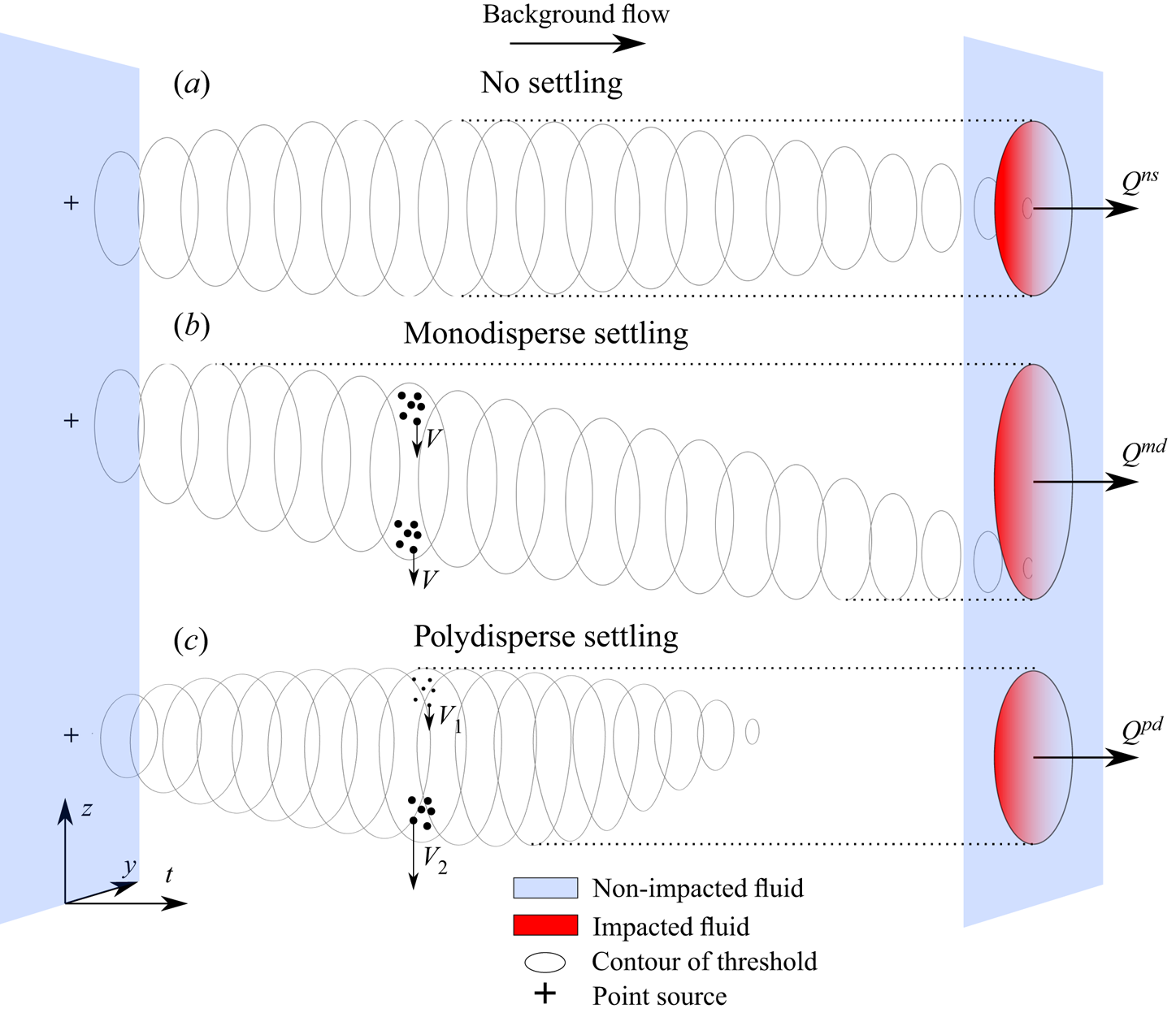
Figure 2. Contours of threshold concentration as a function of time in the absence of settling (a), monodisperse settling (b) and polydisperse (denoted by pd) settling (c). The volume flux  $Q$ of fluid that flows through a region above the concentration threshold depends strongly on settling and polydispersity. Monodisperse settling acts to increase the effective area that parcels of fluid flow through exceeding a concentration threshold. Polydispersity acts to stretch the plume in the vertical direction through differential settling ( $V_1< V_2$), thereby diluting the plume, and reducing the effective area compared with the monodisperse equivalent.
In the absence of settling we therefore find that the volume flux of water that will at some point exceed a certain particle concentration  $C_t$ only depends on the mass flow rate of sediment and the threshold value. Surprisingly, it is independent of the vertical and horizontal turbulent diffusivities, as well as the background velocity. This result can be understood through the following reasoning: the mass of sediment per unit length contained in a vertical slice of the plume is simply set by ${\dot m}/{U}$. Given that the concentration is inversely proportional to the area covered by the plume, it immediately follows that while diffusivity controls how quickly the threshold area is reached, it will not play a role in the area itself as it is entirely controlled by the mass per unit length and the considered threshold. The instantaneous volume of fluid in excess of a threshold value, which we recall to be a Eulerian metric that is constant in time, can easily be calculated for non-settling particles using (4.6) as
 \begin{equation} \mathcal{V}^{ns} = U\int_0^{t_t}A(t)\,{{\rm d}}t = \frac{\dot m^{2}}{16{\rm \pi}\sqrt{\kappa_y\kappa_z}UC_t^{2}}. \end{equation}
It depends quadratically on the ratio of discharged mass flux to concentration threshold, and will therefore be markedly more sensitive to a change in these parameters than the volume flux of fluid that ever exceeds the same threshold.
4.2.2 Monodisperse suspensions
If we now consider a monodisperse suspension of particles with a unique, non-zero settling velocity  $V$, then the volume flux of fluid that will at some point exceed the threshold concentration does not simply depend on the maximum area reached by the plume above the threshold, but also on the settling velocity. This is because as particles settle vertically relative to the horizontal background flow, provided that the height they settle over the maximal area time scale $t_{max}$ is significant, they pass through different parcels of fluid. This increases the effective area that ever exceeded a threshold, a process illustrated in figure 2(b). Quantitatively, this area is the spatial integral of all the ( $y,z$) positions where the plume exceeds the threshold concentration at some time $t\in ]0,t_t]$, which we define as
 \begin{equation} A_q = \iint_{\delta \varOmega}\delta(y,z)\,{{\rm d}}z\,{{\rm d}}y, \end{equation}
where  $\delta (y,z)=1$ where the plume exceeds the concentration $C_t$ at some time $t$, and $\delta (y,z)=0$ elsewhere. The corresponding volume flux of water that will at some point exceed the concentration threshold is simply $Q=UA_q$.
It is anticipated that settling will play a dominant role in controlling the vertical extent of  $\delta (y,z)$ when settling is much faster than the characteristic vertical diffusion velocity for a particular concentration threshold. Let $L_z$ be the maximum vertical extent of the contour of concentration $C_t$,
 \begin{equation} L_z = 2z_t(t_{max},y = 0) = 2\left({\rm e}^{{-}1}\sqrt{\frac{\kappa_z}{\kappa_y}} \frac{\dot m }{{\rm \pi} UC_t}\right)^{{1}/{2}}. \end{equation}
We can then define a characteristic vertical diffusion velocity  $V_z$ for the concentration contour $C_t$ as
 \begin{equation} V_z = \frac{L_z}{t_{max}} = \frac{L_z}{{\rm e}^{{-}1}t_t} = 8\sqrt{{\rm \pi} \,{\rm e}^{1}} \left(\frac{C_t^{2}U^{2}\kappa_z^{3}\kappa_y}{\dot m^{2}}\right)^{1/4}. \end{equation}
Under the condition  $V\gg V_z$, the effective area $A^{md}_q$ (‘md’ stands for ‘monodisperse’) of the monodisperse plume is given by the integral of the plume width at its widest, i.e. $2y_t$, over the vertical extent $Vt$, for $t\in ]0,t_t]$, i.e.
 \begin{equation} A_q^{md} = 2V\int_0^{t_t}y_t(t)\,{{\rm d}}t = \frac{1}{3{\rm \pi}}\sqrt{\frac{1}{6}} \frac{V}{U}\left(\frac{\dot m^{6}}{U^{2}C_t^{6}\kappa_y\kappa_z^{3}}\right)^{{1}/{4}}. \end{equation}
Following the same rationale as for non-settling particles, the volume flux of fluid that is at some point in time above the threshold concentration is therefore
 \begin{equation} Q^{md} = U A_q^{md} = \frac{1}{3{\rm \pi}}\sqrt{\frac{1}{6}}V \left(\frac{\dot m^{6}}{U^{2}C_t^{6}\kappa_y\kappa_z^{3}}\right)^{{1}/{4}}. \end{equation}
 Unlike the result in the absence of settling, the expression (4.14) involves all the parameters of the problem, i.e. both diffusion coefficients, the background velocity, the concentration threshold, the mass flux and the settling velocity. The exponential solution (4.1) is used to directly compute the area from (4.10) across a range of settling velocities  $V$. The results are plotted for the volume flux $Q=UA_q$ in figure 3(a). The volume flux is scaled with the analytical value $Q^{ns}={\rm e}^{-1}({\dot m}/{C_t})$ in the absence of settling, and the settling velocity is scaled with the vertical diffusion velocity of the threshold contour, $V_z$. For small values of $V/V_z$, the volume flux is equal to the analytical solution in the absence of settling (black dashed line, see (4.8)), while for large values of $V/V_z$, the volume flux is equal to the analytical solution in the settling-dominated regime (red dashed line, see (4.14)). Settling only becomes important when $V/V_z \sim 0.1$, and the volume flux converges to the settling-dominated solution when $V/V_z\gtrapprox 1$. The instantaneous volume of fluid in excess of a threshold value remains unchanged in the case of a monodisperse suspension, as settling only acts to translate the sediment downwards, and $\mathcal {V}^{md}=\mathcal {V}^{ns}$.

Figure 3. (a) Volume flux as a function of weight-averaged settling velocity for a monodisperse suspension as well as various levels of polydispersity. A normal distribution of settling speeds is assumed with standard deviation  $\sigma$, defined relatively to the mean settling velocity $\bar V$. The no-settling solution $Q={\rm e}^{-1}({\dot m}/{C_t})$ and monodisperse solution in the limits of strong settling $Q=({1}/{3{\rm \pi} }) \sqrt {\frac {1}{6}}V({\dot m^{6}}/ {U^{2}C_t^{6}\kappa _y\kappa _z^{3}})^{{1}/{4}}$ are shown in black and red dashed lines, respectively. (b) Instantaneous volume $\mathcal {V}$ of fluid above a threshold as a function of weight-averaged settling velocity for a monodisperse suspension as well as various levels of polydispersity. A normal distribution of settling speeds is assumed with standard deviation $\sigma$, defined relatively to the mean settling velocity $\bar V$. The volume $\mathcal {V}$ is expressed relatively to the no-settling solution $\mathcal {V}^{ns}= {\dot m^{2}}/{16{\rm \pi} \sqrt {\kappa _y\kappa _z}UC_t^{2}}$.
4.2.3 Polydisperse suspensions
While the effective area increases linearly with settling velocity in the settling-dominated regime, this assumes that all the particles settle at the same speed. In reality, resuspended sediment always displays a certain level of polydispersity and, thus, a range of settling velocities. In a polydisperse suspension, the vertical extent of the plume at a given time depends not only on vertical diffusion, but also on differential settling. As fine particles settle more slowly than large particles, the plume is stretched in the vertical direction, effectively diluting it, as sketched in figure 2(c). While the PVD of real sediment will depend greatly across different regions of the ocean and the technology used, some general observations can be made on the role of polydisperse settling.
To do so, we consider a normal distribution of settling velocities with mean  $\bar V$ and standard deviation $\sigma$. The probability density function is discretized into 31 equally spaced bins of velocities between $\bar V-4\sigma$ and $\bar V+4\sigma$. As done for monodisperse settling, we compute the effective area for a range of mean settling velocities, with standard deviations $0.05\bar V$, $0.1\bar V$, $0.25\bar V$, $0.5\bar V$ and $1\bar V$.
The results presented in figure 3(a) for the volume flux  $Q=UA_q$, in which we again scale the flux and velocity with $Q^{ns}$ and $V_z$, respectively, reveal that polydispersity does not affect the volume flux in the diffusion dominated regime, but becomes important in the settling-dominated regime. The larger the level of polydispersity (or the larger the standard deviation), the smaller the volume flux of impacted fluid when compared with the monodisperse equivalent. This observation can be generalized to other distributions by considering the characteristic vertical stretch of the plume induced by differential settling. This stretch exceeds the vertical stretch due to diffusion when $\sigma t\gtrsim \sqrt {4\kappa _z t}$. For polydispersity to play a role for a given threshold $C_t$, this transition must occur for $t< t_t$. We thus anticipate that polydispersity affects the volume flux of impacted fluid only when
 \begin{equation} \sigma^{2}\gtrsim \frac{\kappa_z\sqrt{\kappa_z\kappa_y}UC_t}{\dot m}. \end{equation}
This inequality only provides insight into the scaling of the level of polydispersity required for differential settling to play a significant role and cannot be used directly to rule out the role polydispersity in a particular suspension. One should instead directly use the solution of (4.1) combined with (4.10) for the particle settling velocity distribution considered, and compare the results with the monodisperse equivalent with the same weight-averaged settling speed.
The instantaneous volume  $\mathcal {V}$ of fluid above a threshold is also affected by polydispersity. Vertical stretching due to differential settling initially increases the vertical cross-sectional area of the plume, but it also acts to dilute the plume more quickly. This leads to a significant decrease of the instantaneous volume $\mathcal {V}$ compared with the no-settling (and monodisperse) case in the settling-dominated regime, as seen in figure 3(b).
4.3 Maximum horizontal and vertical extent
In this section we consider the furthest horizontal distance  $L$ from the source, as well as the maximum depth below the release point $D$ where the concentration can exceed the threshold value $C_t$. Once again, we build complexity by considering non-settling particles, monodisperse particles and polydisperse suspensions.
4.3.1 Non-settling particles
In the absence of settling, the furthest horizontal distance  $L$ is trivially related to the maximum time $t_t$ (see § 4.1) as
 \begin{equation} L^{ns} = Ut_t = \frac{\dot m}{4{\rm \pi}\sqrt{\kappa_y\kappa_z}C_t}. \end{equation}
Thus, the radial distance around a midwater intrusion where a concentration threshold might be exceeded depends not only on the ratio of discharged mass flux to concentration threshold, but also on ambient turbulent processes. In the absence of settling, the maximum depth below the intrusion where the concentration exceeds a threshold value  $C_t$ is given by $D^{ns} = \max _{0< t< t_t}(z_t'(t,y=0)) = L_z/2$, i.e.
 \begin{equation} D^{ns} = \left({\rm e}^{{-}1}\sqrt{\frac{\kappa_z}{\kappa_y}}\frac{\dot m }{{\rm \pi} UC_t}\right)^{{1}/{2}}. \end{equation}
4.3.2 Monodisperse settling
In the case of monodisperse settling, the furthest horizontal distance  $L$ where the concentration can exceed $C_t$ remains unchanged and $L^{md}=L^{ns}$. However, the maximum depth reached by the plume is directly affected by settling and is given by $D^{md} = \max _{0< t< t_t}(Vt + z_t'(t,y=0))$. In the limit of strong settling, it can be inferred that the depth reached is
 \begin{equation} D^{md} = Vt_t = \frac{V}{U}\frac{\dot m}{4{\rm \pi}\sqrt{\kappa_y\kappa_z}C_t}, \end{equation}
and vertical diffusion plays a negligible role in the depth reached for a given threshold. The furthest distance  $L$ and maximum depth $D$ where the plume exceeds a concentration threshold are plotted in figures 4(a) and 4(b), respectively. The distance $L$ and the depth $D$ are plotted relatively to the distance in the absence of settling (4.16) and the depth $D$ in the absence of settling (4.17), respectively. While the distance $L$ is unaffected by monodisperse settling, the depth reached strongly depends on settling speed, and the role of settling becomes significant when $V/V_z\gtrapprox 0.1$. For small settling speeds, the depth reached converges to the limit in the absence of settling $D^{ns}$ (black dashed line in figure 4b). At large settling velocities, in the monodisperse regime, the depth indeed converges to the settling-dominated limit $D^{md}$ (red dashed line in figure 4b).

Figure 4. (a) Furthest distance  $L$ where the plume can exceed a concentration threshold, relative to $L^{ns}={\dot m}/{4{\rm \pi} \sqrt {\kappa _y\kappa _z}C_t}$. (b) Maximum depth $D$ where the plume can exceed a concentration threshold, relative to $D^{ns}=({\rm e}^{-1}\sqrt {{\kappa _z}/{\kappa _y}}({\dot m }/{{\rm \pi} UC_t}))^{{1}/{2}}$. The black and red dashed lines correspond to the limits of no settling and strong monodisperse settling, respectively. In both (a,b), results for monodisperse suspensions and polydisperse suspensions are shown for various levels of polydispersity, as a function of the mean settling speed $\bar V$.
4.3.3 Polydisperse suspensions
As for the volume flux, we investigate the role of polydispersity on  $L$ and $D$ by considering a normal distribution of particle settling velocities, and vary the standard deviation $\sigma$ (see § 4.2.3 for details). The furthest distance $L$ and maximum depth $D$ are plotted in figure 4 for various levels of polydispersity. Unlike the monodisperse case, polydispersity tends to decrease the furthest distance reached by the plume for a given concentration threshold. As for the volume flux, this is due to the fact that differential settling leads to an effective vertical stretching of the plume, thereby reducing its concentration. At low mean settling velocities, settling does not play a role and the distance is identically equal to that of the no-settling case. Interestingly, the mean settling velocity is a poor indicator of when settling will start affecting the distance $L$, as the mean velocity at which settling becomes important depends on the standard deviation. Indeed, mean settling plays no role in $L$, as shown in the monodisperse case, and it is only the increase in differential settling (which is directly proportional to the standard deviation) that promotes the decrease in $L$. Thus, the reason why $L$ decreases with $\bar V$ in figure 4(a) is simply due to our choice to vary $\sigma$ proportionally to $\bar V$. Figure 4(a) demonstrates that polydispersity plays a central role in setting the maximum distance away from a discharge where a concentration threshold might be exceeded, and modelling efforts that assume a unique settling velocity risk overestimating markedly the radial reach of impact.
Contrary to  $L$, the maximum depth $D$ reached for a given threshold depends, like the volume flux $Q$, on both the mean settling velocity and on the level of polydispersity. There, polydispersity acts to reduce the depth reached relative to the monodisperse case by stretching and thereby diluting the plume in the vertical direction. Interestingly, the role of polydispersity appears to decrease at high values of the standard deviation. This is because increasing the standard deviation leads to stronger vertical dilution, reducing the concentration, yet also leading to higher fractions of sediment settling at high velocities, thus reaching further depths more quickly. Differential settling can be seen as a linear dilution process in time, unlike diffusion which goes with the square root of time. It is therefore reasonable to assume that for large levels of polydispersity, the increase in maximum settling speed is compensated by the increase in differential settling, cancelling out the role of increasing polydispersity. The role of polydispersity on setting the depth $D$ is therefore less critical than on setting the furthest distance reached $L$.
$L$.
4.4 Deposition rate and deposition area
The previous analysis focused on the interaction of the plume with the water column. Eventually, particles will settle through the water column to deposit on the seabed, potentially causing a different form of environmental impact. An individual particle settling at an effective settling velocity  $V$ will reach the seabed at $t_s = {H_r}/{V}$, where $H_r$ is the height above the seabed at which the plume intrudes horizontally upon reaching a point of neutral buoyancy following the buoyancy-driven phase. Given that $H_r$ is typically $\mathcal {O}(10^{3})$ m and $V$ is expected to be in the range $\mathcal {O}(10^{-5})$ to $\mathcal {O}(10^{-3})$ m s $^{-1}$, $t_s$ can be in the range $\mathcal {O}(10)$ days to $\mathcal {O}(1000)$ days. After such long times, the plume will have diffused laterally and stretched vertically, as a result of both diffusion and differential settling, by several hundreds of metres, resulting in very weak concentration gradients. The plume will have experienced considerable vertical stretching as a result of differential settling, with some particles having reached the seabed after a few days, and some particles having settled only a few tens of metres over that time span.
Even as a first-order approximation, it is evident that the assumptions made in the advection–diffusion-settling model break down when considering the times associated with deposition of the midwater plume. In theory, the method can be used to estimate deposition rates and areas of the seabed that experience a certain instantaneous deposition rate threshold. Dispersion due to vertical variability in current heading and magnitude, however, will transport particles of different settling velocities in different regions and contribute much more significantly to the evolution of the plume on deposition time scales. In addition, the ability of the model to predict deposition rates at the seabed is only of practical use if deposition can be integrated in time in order to obtain a Eulerian map of the deposition. This implies that the location on the seabed where the plume lands can be predicted through knowledge of the ocean currents. It is highly unrealistic that knowledge of the ocean currents can be had with sufficient accuracy and over sufficient lengths of time that the trajectory of the plume can be predicted. This trajectory would also have to be calculated for many groups or bins of particle sizes. Indeed, any model that discretizes the PVD needs to consider a PVD resolved enough that vertical turbulent diffusion dominates over differential settling within the bin. A given bin of mean settling velocity  $\bar V$ and width $\Delta V$ needs to satisfy that turbulent diffusion still dominates over vertical stretching at time $t_s$, i.e. that $\sqrt {\kappa _z({H_r}/{\bar V})}\gg \Delta V({H_r}/{V})$, or ${\Delta V}/{V}\ll \sqrt {{\kappa _z}/{H_r\bar V}}$. For typical values of $\kappa _z$, $H_r$ and $\bar V$, ${\Delta V}/{V}\ll 1$, suggesting that very highly resolved PVDs need to be considered, or vertical stretching needs to be alternatively modelled. Provided that the discretization condition is met, then the maximum deposition rate for a given bin can be estimated from (4.1) as
 \begin{equation} q_{max} \approx \frac{\dot m^{ * }\bar V^{2}}{4{\rm \pi} \sqrt{\kappa_y\kappa_z}UH_r}, \end{equation}
where  $\dot m^{*}$ is the discharged mass flow rate of particles within the considered settling velocity bin.
Thus, the maximum possible deposition rate for a given bin is linearly proportional to the discharge mass flow rate within the bin, and inversely proportional to the background velocity, intrusion height above the seabed and square root of the product of the diffusivities. Most importantly, it is proportional to the square of the settling speed, which suggests that coarse particles are more likely to exceed a given threshold of deposition rate than fine particles. Note, however, that the larger the particle settling velocity, the smaller the relative bin width  $\Delta V/\bar V$ needs to be and, thus, the smaller $\dot m^{*}$ relative to the total discharge mass flow rate $\dot m$. While beyond the scope of the present work, an interesting question is the role played by the bottom boundary layer on the eventual deposition of sediment from midwater plumes. Evidence of highly elevated turbulent diffusion in the bottom mixed layer in the Clarion- Clipperton zone (Reference van Harenvan Haren, 2018) suggest that upon reaching the bottom mixed layer, sediment will be initially more quickly diffused towards the seabed, but may also deposit more slowly as turbulence maintains sediment in suspension for longer. The evolution of collector near-seabed plumes, which can give insight into this problem, is the topic of Part 2.
5. Application
We now consider a reference DSM scenario around which we vary various parameters and comment on the resulting changes to the volume flux  $Q$ of ambient fluid that ever exceeds a concentration threshold, the maximum distance $L$ away from the source that exceeds a concentration threshold, the maximum depth $D$ reached by the plume where a concentration threshold is exceeded, and the instantaneous volume $\mathcal {V}$ in excess of a concentration threshold. The maximum deposition rate at the seabed is not considered as its applicability is unclear even as a first-order estimate. The reference scenario is not meant to be most representative of DSM operations, it simply serves as a platform around which we vary the parameters of interest. In all cases, we take $\kappa _y =1$ m $^{2}$ s $^{-1}$, $U=0.05$ m s $^{-1}$. For the reference case, we take $\kappa _z=10^{-5}$ m $^{2}$ s $^{-1}$, $\dot m = 100$ kg s $^{-1}$ and $C_t=100\,\mathrm {\mu }$g l $^{-1}$. We then consider various vertical diffusivities $\kappa _z$, discharge mass flow rates $\dot m$ and concentration (deposition rate) thresholds $C_t$ ( $q_t$). We additionally consider three different polydisperse suspensions each with its own PVD $P(V)$. The PVDs are derived from a corresponding particle size distribution (PSD) that is either centred, skewed towards small particles or skewed towards large particles. We use Stokes’ law and assume a constant particle density $\rho _p =2600$ g l $^{-1}$ to relate particle diameter to particle settling velocity. For the PSDs, we assume a beta distribution of particles of diameters ranging from 5 to 100 $\mathrm {\mu }$m, with shape parameters $(\alpha,\beta )=(4,4)$ for the reference scenario (mean particle diameter $\bar d_p =52.5\,\mathrm {\mu }$m), $(\alpha,\beta )=(2,7)$ for the small particles scenario (mean particle diameter $\bar d_p =26.4\,\mathrm {\mu }$m) and $(\alpha,\beta )=(7,2)$ for the large particles scenario (mean particle diameter $\bar d_p =78.6\,\mathrm {\mu }$m). As described in § 3, the PVDs are discretized into $N$ particle velocity bins. The discretized PSDs and PVDs for the three scenarios are shown in figure 5. We note that while PVDs could have been directly defined for all three scenarios without the associated PSDs and the use of Stokes’ law, it is interesting to discuss the variability of the extent metrics as a function of the mean particle diameter size, as it used most often to describe the properties of particles in sediment transport problems.

Figure 5. Discretized PSDs and PVDs of the three suspensions considered. We assume particles ranging from 5 to 100  $\mathrm {\mu }$m. The PVDs are derived from the PSDs using Stokes’ law. The reference scenario admits a beta distribution of particle sizes with shape parameters $(\alpha,\beta )=(4,4)$. Particle size distributions skewed towards smaller and larger particles are then considered with shape parameters $(\alpha,\beta )=(2,7)$ and $(\alpha,\beta )=(7,2)$, respectively.
The four metrics  $Q$,
$Q$,  $L$,
$L$,  $D$ and $\mathcal {V}$ are calculated for all nine scenarios considered and the parameters and results are summarized in table 1. The results are further synthesized in figure 6 for each metric. We specifically do not derive mean or median extent metrics as it would imply that the selection of parameters around the reference scenario is statistically representative of DSM operations, which it is not intended to be. Instead, we note that the first three metrics span approximately two orders of magnitude. The Eulerian metric of the instantaneous volume of impacted fluid, which we recall might hold some relevance to swimming organisms, spans four orders of magnitude, owing to its quadratic dependence on the amount of sediment discharged, and the concentration threshold (see (4.9)). In the case of the midwater plume, the discharge mass flow rate and the concentration threshold are the two parameters that most influence the extent metrics. As can be inferred from the linearity of the transport equation, increasing the mass flow rate of discharged sediment plays the same role as decreasing the concentration threshold, such that scenarios b2 and c2 produce identical extent metrics. The vertical diffusivity plays almost no role in setting the extent metrics for the cases considered, confirming that vertical dilution in midwater plumes of polydisperse sediment is almost entirely controlled by differential settling, not turbulent vertical mixing. It follows that the PVD plays a significant role on the volume flux $Q$, distance $L$ and instantaneous volume $\mathcal {V}$. The PVD with the smaller mean particle diameter experiences weaker differential settling, allowing it to travel further and occupy a larger volume above the threshold, yet the reduced mean settling yields a smaller volume flux of impacted fluid and reduces the maximum depth reached. Conversely, the plume with the larger mean particle diameter experiences stronger settling and stronger differential settling, leading to an increase in the volume flux of impacted fluid and an increase in the depth reached, but a reduction in the distance reached and the instantaneous volume. Depending on the criteria for impact, a change in the properties of the sediment can therefore lead to opposing effects on the magnitude of the impact.

Figure 6. Synthesis plot of DSM scenarios and associated extent metrics.
Table 1. Synthesis table of DSM scenarios and associated extent metrics for various values of the vertical turbulent diffusivity  $\kappa _z$, sediment mass flow rate $\dot m$, concentration threshold $C_t$, mean particle diameter $\bar {d}_p$. The extent metrics are the volume flux $Q$ of ambient fluid that ever exceeds the concentration threshold, the maximum distance $L$ away from the source where the concentration threshold is exceeded, the maximum depth $D$ below the intrusion where the concentration threshold is exceeded, and the instantaneous volume $\mathcal {V}$ in excess of the concentration threshold. Bold values represent parameters which have been changed compared to the reference scenario.

It is also particularly important to note that the instantaneous volume of fluid above a threshold cannot alone be used to characterize the impact to the water column over any period of time. The volume flux  $Q$ is the metric that best characterizes this impact, and the volume of impacted fluid is proportional to the duration of operation considered. For instance, we see that the yearly impacted volume in the reference case is $Q\,\times\, 1yr = 1.5\,\times\, 10^{3}$ km $^{3}$, which is two orders of magnitude larger than the instantaneous volume above the threshold. Over a 10-year operation, the impacted volume would be three orders of magnitude larger than the instantaneous volume. On the other hand, the volume of fluid that exceeds the concentration threshold at any particular point in time is, in this model, a constant, owing to the fact that the contours of concentration of the plume reach a steady state through the balance of advection, diffusion and settling.
6. Conclusion
We solved simplified transport equations that model midwater sediment plumes in a regime dominated by advection in the direction of background currents, and turbulent diffusion in the plane normal to the direction of advection. We used the solution to derive analytical formulas for key extent metrics, mainly the volume flux of fluid that ever exceeds a concentration threshold, the furthest distance from the source and maximum depth where this threshold is exceeded, and the instantaneous volume of fluid where a threshold concentration is exceeded. How the environmental impact scales with these extent metrics is an open question in environmental science, and impact is likely to depend on a multitude of factors, such as exposure time, the nature of the impacted biomarker and many others. Extent metrics derived specifically for a given impact marker can readily be derived using this model as the interaction between plumes and the ocean environment become better understood.
While this simple model does not account for the role of spatial inhomogeneity of background currents and turbulence, it allowed us to derive first-order approximations of extent metrics that are otherwise particularly challenging to obtain using more accurate methods, such as large-scale numerical simulations. Given the considerable uncertainty that remains as to the nature of transport in the deep ocean, the role of meso- and submesoscale eddies, internal waves and mixing hotpots, these formulas are meant to derive order of magnitude estimates of the extent of midwater plumes, and gain insight into the role of advection, diffusion and settling.
Of critical importance is the recognition that the volume of fluid that ever exceeds a concentration threshold is given by the time integral of the flux of fluid to ever exceed that threshold, and is therefore a quantity that increases with time. This is in contrast to the instantaneous volume of fluid that exceeds a threshold, which is expected to reach a quasi-steady state under slowly varying ocean conditions, and can thus be understood as relatively constant in time. It can neither be said that the concentration in the water column is ever increasing, nor can it be said that the impact will reach an asymptote and become independent of the duration of a DSM operation. Differentiating between Lagrangian and Eulerian metrics of impact is critical.
We find that in the absence of settling, the flux of fluid to ever exceed a threshold depends only on the mass of sediment being discharged per unit time and the concentration threshold. The volume flux when considering a monodisperse suspension is unaffected by settling up to a characteristic settling velocity, which represents the transition from a diffusion-dominated plume to a settling-dominated plume. Around and above this characteristic settling velocity, the volume flux increases with settling, and depends not only on the discharged mass and threshold considered, but also on the background velocity and turbulent diffusivities. In the limit of large settling, an analytical formula for the flux can be derived that depends linearly on the settling speed. We further explore the role of polydispersity by considering normal distributions of settling velocities with a range of standard deviations. We find that, in the settling-dominated regime, an increase in standard deviation leads to a decrease in volume flux relative to the equivalent monodisperse suspension.
The furthest distance from the discharge where the plume exceeds a threshold value does not depend on the settling velocity in monodisperse suspensions, but decreases with the level of polydispersity, i.e. with increasing spread of the PVD. The maximum depth reached depends weakly on the mean settling speed in the diffusion-dominated regime, and strongly on the mean settling velocity in the settling-dominated regime. In the latter, polydispersity acts to reduce the maximum depth reached for a threshold. This effect is, however, less pronounced than for the volume flux as increasing polydispersity increases both stretching and dilution of the plume, as well as the maximum settling speed, allowing the plume to reach lower depths quicker. Finally, while the model cannot be used to determine a time integral of any of the seabed quantities, as that would require solving for the transport by actual flow fields in the ocean to determine where on the seabed the plume lands, it can be used to estimate the concentration of the plume at the seabed as a result of settling and, therefore, to estimate the maximum instantaneous deposition rates at the seabed. This calculation can only be carried out under the assumption that differential settling is dominated by vertical diffusion over the time scales considered, and, thus, can only be applied to a narrow bin of particle settling velocities.
The instantaneous volume of fluid that exceeds a concentration threshold varies quadratically with the ratio of mass flow rate of sediment to concentration threshold, when polydispersity is not considered. This Eulerian metric is therefore highly sensitive to the choice of threshold value for impact. Over the time scale of a mining operation, the total volume of fluid that ever exceeds a threshold is several orders of magnitude larger than the instantaneous volume above a threshold.
Funding Statement
T.P. acknowledges funding through ONR grant N000141812762 and through the Benioff Ocean Initiative (the funders had no role in any aspects of the research).
Declaration of Interests
The authors declare no conflict of interest.
Author Contributions
R.O. developed the model and produced the results. T.P. created the research plan. R.O and T.P. led the writing of the manuscript, to which M.A and C.M.R also contributed. M.A. and C.M.R. provided physical guidance for analysis and case studies.
Data Availability Statement
Raw data are available from the corresponding author (R.O.).
Ethical Standards
The research meets all ethical guidelines, including adherence to the legal requirements of the study country.


 Open access
Target article
Advection–diffusion settling of deep-sea mining sediment plumes. Part 2. Collector plumes
Related commentaries (1)
Advection-diffusion-settling of deep-sea mining sediment plumes. Part 1: Midwater plumes