


1. Introduction
The non-Newtonian behaviour of turbulent polymer solutions results from the stretching of polymer molecules dissolved in the fluid. A detailed understanding of the statistics of polymer stretching in turbulent flows is, therefore, essential to explain phenomena such as turbulent drag reduction (Graham Reference Graham2014; Benzi & Ching Reference Benzi and Ching2018; Xi Reference Xi2019) and elastic turbulence (Steinberg Reference Steinberg2021). On the flip side, extreme stretching causes the mechanical scission of polymers, following which all non-Newtonian effects are lost (Soares Reference Soares2020). To accurately model scission and the consequent loss of viscoelasticity, we must understand how the turbulent flow stretches out individual polymers to large extensions.
The strain rate in a turbulent flow fluctuates in magnitude and orientation. In addition, vorticity constantly rotates the polymers and prevents them from persistently aligning with the stretching eigendirection of the strain rate tensor. Nonetheless, Lumley (Reference Lumley1973) predicted that a turbulent flow can stretch polymers, if the product of the mean-square strain rate and its Lagrangian integral time exceeds the inverse of the elastic relaxation time of the polymers. The Lagrangian numerical simulations of Massah et al. (Reference Massah, Kontomaris, Schowalter and Hanratty1993) confirmed the unravelling of individual bead–spring chains in a turbulent channel flow, while Groisman & Steinberg (Reference Groisman and Steinberg2001) provided experimental evidence of this phenomenon in elastic turbulence: the transition from a laminar shear flow to a chaotic flow was found to coincide with a dramatic increase in the polymer-induced shear stress.
A systematic theory of polymer stretching in turbulent flows was developed by Balkovsky, Fouxon & Lebedev (Reference Balkovsky, Fouxon and Lebedev2000, Reference Balkovsky, Fouxon and Lebedev2001) and Chertkov (Reference Chertkov2000) using the methods of dynamical systems. One of the main results is that the end-to-end extension  $R$ of the polymer has a stationary probability density function (p.d.f.) $p(R)$ that behaves as a power law $R^{-1-\alpha }$ for $R$ between the equilibrium and contour lengths of the polymer. The exponent $\alpha$ is a function of the Weissenberg number $\mathit {Wi}$, defined as the product of the Lyapunov exponent of the flow and the polymer relaxation time; this relationship is expressed in terms of the Cramér function that describes the large deviations of the stretching rate of the flow. Note that the power-law behaviour of $p(R)$ is a distinctive feature of turbulent flows – the distribution of polymer extensions remains broad even at large strain rates – and is not observed in laminar, extensional flows (Perkins, Smith & Chu Reference Perkins, Smith and Chu1997; Nguyen & Kausch Reference Nguyen and Kausch1999; Schroeder Reference Schroeder2018).
The power-law behaviour of the p.d.f. of  $R$ has been confirmed in various flow configurations: experimentally by direct observation of individual polymers in elastic turbulence (Gerashchenko, Chevallard & Steinberg Reference Gerashchenko, Chevallard and Steinberg2005; Liu & Steinberg Reference Liu and Steinberg2010, Reference Liu and Steinberg2014); and numerically in shear turbulence (Eckhardt, Kronjäger & Schumacher Reference Eckhardt, Kronjäger and Schumacher2002; Puliafito & Turitsyn Reference Puliafito and Turitsyn2005), in two- and three-dimensional isotropic turbulence (Boffetta, Celani & Musacchio Reference Boffetta, Celani and Musacchio2003; Watanabe & Gotoh Reference Watanabe and Gotoh2010; Gupta, Perlekar & Pandit Reference Gupta, Perlekar and Pandit2015; Rosti, Perlekar & Mitra Reference Rosti, Perlekar and Mitra2023), and in turbulent channel and pipe flows (Bagheri et al. Reference Bagheri, Mitra, Perlekar and Brandt2012; Serafini et al. Reference Serafini, Battista, Gualtieri and Casciola2022). This study further investigates the power-law behaviour of $p(R)$ by examining (i) how polymer stretching is affected by the extreme velocity gradient fluctuations that characterize turbulence, and (ii) how the p.d.f. of $R$ evolves from an initial distribution of coiled polymers to its stationary profile.
Typically, the contour length of the polymer is smaller than the viscous scale of the turbulent flow, so polymer deformation is determined entirely by the statistics of the velocity gradient (Ilg et al. Reference Ilg, De Angelis, Karlin, Casciola and Succi2002; Stone & Graham Reference Stone and Graham2003; Zhou & Akhavan Reference Zhou and Akhavan2003; Gupta, Sureshkumar & Khomami Reference Gupta, Sureshkumar and Khomami2004; Terrapon et al. Reference Terrapon, Dubief, Moin, Shaqfeh and Lele2004; Peters & Schumacher Reference Peters and Schumacher2007). It is natural, therefore, to consider simplifying the simulation of polymer stretching by using a random velocity gradient model with appropriate statistics. This would facilitate the testing and development of advanced polymer models, beyond the simple dumbbell or freely-jointed chain, by avoiding expensive direct numerical simulations (DNS) of the carrier flow. However, one must first answer the question: does stochastic modelling of the turbulent flow modify, in a fundamental way, the stretching dynamics of polymers?
In the broader context of the turbulent transport of anisotropic particles, several studies have shown that particle-orientation dynamics cannot be explained fully by using Gaussian models of the velocity gradient (see e.g. Pumir & Wilkinson Reference Pumir and Wilkinson2011; Chevillard & Meneveau Reference Chevillard and Meneveau2013; Gustavsson, Einarsson & Mehlig Reference Gustavsson, Einarsson and Mehlig2014; Allende, Henry & Bec Reference Allende, Henry and Bec2018; Anand, Ray & Subramanian Reference Anand, Ray and Subramanian2020). Meanwhile, for single-polymer dynamics, Gaussian velocity gradient models have undoubtedly been useful in gaining a qualitative understanding of stretching statistics (e.g. Shaqfeh & Koch Reference Shaqfeh and Koch1992; Mosler & Shaqfeh Reference Mosler and Shaqfeh1997; Chertkov Reference Chertkov2000; Martins Afonso & Vincenzi Reference Martins Afonso and Vincenzi2005; Puliafito & Turitsyn Reference Puliafito and Turitsyn2005; Vincenzi et al. Reference Vincenzi, Watanabe, Ray and Picardo2021). To our knowledge, however, the effect of the strongly non-Gaussian fluctuations of a turbulent velocity gradient on the statistics of  $R$, and in particular on the dependence of $\alpha$ upon $\mathit {Wi}$, has not yet been investigated. With this aim, we carry out Lagrangian numerical simulations of finitely extensible nonlinear elastic (FENE) dumbbells in three-dimensional isotropic turbulence, as well as in a Gaussian model of the velocity gradient, and compare the statistics of $R$. This investigation has relevance beyond stochastic modelling, because flows without extreme strain rates arise naturally in the context of polymer solutions – wherein polymer feedback forces suppress extreme velocity gradient fluctuations (Perlekar, Mitra & Pandit Reference Perlekar, Mitra and Pandit2010; Watanabe & Gotoh Reference Watanabe and Gotoh2013; ur Rehman, Lee & Lee Reference ur Rehman, Lee and Lee2022).
So far, most studies have focused on the stationary statistics of polymer extensions. However, the transient dynamics is important in situations where polymer scission occurs and the long-time stationary state may never be reached (Soares Reference Soares2020). In addition, the finite-time statistics of polymer stretching is relevant to experimental measurements, which are necessarily limited in their duration, as well as to the calibration of numerical simulations. The characteristic time required for polymers to equilibrate in a turbulent flow has been studied in stochastic models (Martins Afonso & Vincenzi Reference Martins Afonso and Vincenzi2005; Celani, Puliafito & Vincenzi Reference Celani, Puliafito and Vincenzi2006) and isotropic turbulence (Watanabe & Gotoh Reference Watanabe and Gotoh2010). A significant slowing down of the stretching dynamics has been found near the coil–stretch transition. This phenomenon is reminiscent of the slowing down observed in an extensional flow (Gerashchenko & Steinberg Reference Gerashchenko and Steinberg2008), but has a different origin. Specifically, it is not a consequence of the conformation hysteresis typical of extensional flows (Schroeder et al. Reference Schroeder, Babcock, Shaqfeh and Chu2003; Schroeder, Shaqfeh & Chu Reference Schroeder, Shaqfeh and Chu2004), but rather arises from the strong heterogeneity of polymer configurations in the vicinity of the coil–stretch transition (Celani et al. Reference Celani, Puliafito and Vincenzi2006). Other than the equilibration time, little is known about how the p.d.f. of polymer extension approaches its asymptotic shape and, in particular, whether or not the power-law behaviour appears at earlier times. Here, this issue is studied by means of Lagrangian simulations of single-polymer dynamics in three-dimensional isotropic turbulence; simulations for both a dumbbell and a bead–spring chain are compared. In addition, the numerical results are explained by using a Fokker–Planck equation for the time-dependent p.d.f. of  $R$.
$R$.
The dumbbell model of polymers is presented in § 2, along with a description of the Lagrangian simulations that form the basis of this study. The random and turbulent carrier flows are also described there. Section 3 focuses on the stationary p.d.f. of polymer extensions. In § 3.1, the theory of Balkovsky et al. (Reference Balkovsky, Fouxon and Lebedev2000) and Chertkov (Reference Chertkov2000) is recalled briefly, and is illustrated by using a renewing Couette flow. Section 3.2 then examines the effect of the non-Gaussian statistics of a turbulent velocity gradient on polymer stretching. Section 4 is devoted to understanding the temporal evolution of the p.d.f. of polymer extensions, with the aid of a stochastic model. We then verify, in § 5, that the results obtained for the elastic dumbbell remain true even for chains with a larger number of beads. Finally, we conclude in § 6 with a summary of our study and a discussion of its implications.
2. Lagrangian simulations in random and turbulent flows
2.1. Dumbbell model
We primarily model polymer molecules using the FENE dumbbell model (Bird et al. Reference Bird, Curtiss, Armstrong and Hassager1987; Öttinger Reference Öttinger1996; Graham Reference Graham2018). With  $\tau$ as the relaxation time of the polymer, $R_{{eq}}$ as the equilibrium root-mean-square (r.m.s.) end-to-end length, and $R_m$ as the maximum length, the dynamics of the end-to-end separation vector $\boldsymbol {R}$ in $d$ dimensions satisfies
 \begin{equation} \frac{\mathrm{d}\boldsymbol{R}}{\mathrm{d}t}=\boldsymbol{\kappa}(t)\boldsymbol{\cdot}\boldsymbol{R}-f(R)\,\frac{\boldsymbol{R}}{2 \tau} +\sqrt{\frac{R_{{eq}}^2}{\tau d}}\,\boldsymbol{\xi}(t), \end{equation}
where  $\kappa _{ij}=\boldsymbol {\nabla }_j u_i$ is the velocity gradient at the location of the centre of mass of the polymer, $f(R)=(1-R^2/R_m^2)^{-1}$ defines the FENE spring force, and $\boldsymbol {\xi }(t)$ is $d$-dimensional white noise that accounts for thermal fluctuations. This noise would also make an appearance in the equation of motion for the centre of mass. However, its effect on the transport of the dumbbell is very small compared to the advection by the turbulent carrier flow and thus may be neglected. The motion of the centre of mass of the polymer is therefore treated like that of a tracer.
Given a Lagrangian time series of  $\boldsymbol {\kappa }(t)$, (2.1) is integrated using the Euler–Maruyama method supplemented with the rejection algorithm proposed by Öttinger (Reference Öttinger1996), which rejects those time steps that yield extensions greater than $R_m(1-\sqrt {\mathrm {d}t/10})^{1/2}$. Since the velocity gradient fluctuates, the numerical integration of (2.1) does not present the same difficulties as in the case of a laminar extensional flow, and more sophisticated integration methods are not necessary. We have indeed checked that only a negligible fraction of time steps is rejected over a simulation.
Throughout this paper, we study the dumbbell model with  $R_{{eq}}=1$ and $R_m=110$. The elastic relaxation time $\tau$ defines the non-dimensional Weissenberg number, $\mathit {Wi} \equiv \lambda \tau$, where $\lambda$ is the maximum Lyapunov exponent of the carrier flow. The Weissenberg number provides a non-dimensional measure of the elasticity of the polymer, with high- $\mathit {Wi}$ polymers being easily extensible. We consider a wide range of $\mathit {Wi}$, from 0.3 to 40.
Note that while the dumbbell model (2.1) is used in most of this study, we do show in § 5 that our results also hold true for bead–spring chains.
2.2. Turbulent carrier flow
To study polymer stretching in a turbulent flow, we use a database of Lagrangian trajectories from DNS of homogeneous isotropic incompressible turbulence (at Taylor-microscale Reynolds number  ${Re}_\lambda \approx 111$), generated at ICTS, Bangalore (James & Ray Reference James and Ray2017). The DNS solve the incompressible Navier–Stokes equations, discretized on a periodic cube, using a standard fully-dealiased pseudo-spectral method with $512^3$ grid points. Time integration is performed using a second-order slaved Adams–Bashforth scheme. The motion of $9\times 10^5$ tracers is calculated using a second-order Runge–Kutta method for time integration; the fluid velocity at the location of a tracer is obtained from its value on the grid using trilinear interpolation. The velocity gradient $\boldsymbol {\nabla }\boldsymbol {u}$ is calculated along these trajectories and stored at intervals $0.11 \tau _\eta$, where $\tau _\eta$ is the Kolmogorov time scale (given below). These Lagrangian data provide the values of $\boldsymbol {\kappa }(t)$ for the integration of (2.1) along $9\times 10^5$ trajectories, allowing us to obtain good statistics of single-polymer stretching dynamics.
The Lyapunov exponent of the flow, required for defining  $\mathit {Wi}$, is computed from these trajectories via the continuous $QR$ method, implemented using an Adams–Bashforth projected integrator along with the composite trapezoidal rule (for further details, see Dieci, Russell & Van Vleck Reference Dieci, Russell and Van Vleck1997). We find $\lambda =0.136/\tau _\eta$, which is compatible with previous simulations of isotropic turbulence (Bec et al. Reference Bec, Biferale, Boffetta, Cencini, Musacchio and Toschi2006). We also estimate the Lagrangian correlation time scales of strain rate and vorticity in the turbulent flow, $\tau _{S}$ and $\tau _\varOmega$, which serve as inputs to the Gaussian random model described in the next subsection. The rate-of-strain and rotation tensors are defined as ${\boldsymbol{\mathsf{S}}}=(\boldsymbol {\nabla }\boldsymbol {u}+\boldsymbol {\nabla }\boldsymbol {u}^{\rm T})/2$ and $\boldsymbol {\varOmega }=(\boldsymbol {\nabla }\boldsymbol {u}-\boldsymbol {\nabla }\boldsymbol {u}^{\rm T})/2$, respectively. The autocorrelation functions of $S_{11}$ and $\varOmega _{12}$ are calculated and found to display an approximately exponential decay. Integrating these functions yields the integral time scales $\tau _{S}=2.20\,\tau _\eta$ and $\tau _\varOmega =8.89\,\tau _\eta$, in agreement with previous numerical simulations at comparable $R_\lambda$ (Yeung Reference Yeung2001). The Kolmogorov time scale $\tau _\eta$ is determined from $S_{11}$, using isotropy, as $\tau _\eta =({15\langle S_{11}^2\rangle })^{-1/2}=3.72\times 10^{-2}$.
2.3. Gaussian random velocity gradient
One of the goals of this study is to compare the stretching of polymers in a turbulent flow to that in a flow with Gaussian statistics, in order to determine the effect of extreme-valued fluctuations of the turbulent velocity gradient. For this, we use a Gaussian random velocity gradient model to generate a time series of  $\boldsymbol {\kappa }(t)$ for each polymer trajectory. Following Brunk, Koch & Lion (Reference Brunk, Koch and Lion1997), we take $\boldsymbol {\kappa }(t)={\boldsymbol{\mathsf{S}}}(t)+\boldsymbol {\varOmega }(t)$, with
 \begin{equation} \boldsymbol{\mathsf{S}}=\sqrt{3}\,A \begin{pmatrix} \frac{2\zeta_1}{\sqrt{3}} & \zeta_3 & \zeta_4\\ \zeta_3 & -\frac{\zeta_1}{\sqrt{3}}+\zeta_2 & \zeta_5\\ \zeta_4 & \zeta_5 & -\frac{\zeta_1}{\sqrt{3}}-\zeta_2 \end{pmatrix}, \quad \boldsymbol{\varOmega}=\sqrt{5}\,A \begin{pmatrix} 0 & \varpi_1 & \varpi_2\\ -\varpi_1 & 0 & \varpi_3\\ -\varpi_2 & -\varpi_3 & 0 \end{pmatrix}, \end{equation}
where  $A$ determines the magnitude of the velocity gradient, and $\zeta _i(t)$ ( $i=1,\dots,5$) and $\varpi _i(t)$ ( $i=1,2,3$) are independent zero-mean unit-variance Gaussian random variables, with exponentially decaying autocorrelation functions and integral times $\tau _S$ and $\tau _\varOmega$, respectively. Therefore, $S_{ij}$ and $\varOmega _{ij}$ are Gaussian variables such that $\langle S_{ij}\rangle =\langle \varOmega _{ij}\rangle =0$,
 \begin{equation} \langle S_{ik}(t)\,S_{jl}(0)\rangle = 3A^2 (\delta_{ij}\delta_{kl}+\delta_{il}\delta_{jk}-\tfrac{2}{3}\delta_{ik} \delta_{jl}) {\rm e}^{{-}t/\tau_S} \end{equation}
and
 \begin{equation} \langle \varOmega_{ik}(t)\,\varOmega_{jl}(0)\rangle = 5A^2 (\delta_{ij}\delta_{kl}-\delta_{il}\delta_{jk}) {\rm e}^{{-}t/\tau_\varOmega}. \end{equation}
As a consequence,  $\langle \varOmega _{ij}\varOmega _{ij}\rangle =\langle S_{ij}S_{ij}\rangle$, which reproduces the relation $\nu \langle \omega ^2\rangle =\langle \epsilon \rangle$, where $\omega$ is the vorticity and $\epsilon$ is the energy dissipation rate (Frisch Reference Frisch1995). We take $\tau _S$ and $\tau _\varOmega$ to be the same as in the turbulent flow (§ 2.2), and generate $\zeta _i$ and $\varpi _i$ using the algorithm of Fox et al. (Reference Fox, Gatland, Roy and Vemuri1988). Furthermore, we set the coefficient $A= 2.538$ so as to obtain approximately the same Lyapunov exponent $\lambda$ as in the turbulent flow. As a consequence, the Kubo number ${Ku}=\lambda \tau _S$ is also nearly the same in the turbulent and Gaussian flows.
3. Stationary statistics of polymer stretching
We begin our study by considering the long-time, statistically stationary distribution of the end-to-end extension of polymers. We first recall the large deviations theory of Balkovsky et al. (Reference Balkovsky, Fouxon and Lebedev2000) and Chertkov (Reference Chertkov2000), which not only predicts a power-law tail in the p.d.f. of  $R$, but also provides a way to calculate the corresponding exponent for any chaotic carrier flow, given sufficient knowledge of its dynamical properties. We illustrate the predictive capability of the theory for a simple, analytically specified, renewing flow. Unfortunately, direct application of the theory to turbulent flows is impractical, and one must typically resort to approximations, such as considering the turbulent flow to be decorrelated in time. Such considerations will naturally lead us to examine how and to what extent the time-correlated, non-Gaussian nature of turbulent flow statistics impacts polymer stretching.
3.1. Large deviations theory: illustration for a renewing flow
The theory of Balkovsky et al. (Reference Balkovsky, Fouxon and Lebedev2000) and Chertkov (Reference Chertkov2000) is recalled here in terms of the generalized Lyapunov exponents, rather than the Cramér function of the strain rate; the two properties are equivalent and related via a Legendre transform (see Boffetta et al. Reference Boffetta, Celani and Musacchio2003). If  $\boldsymbol {\ell }(t)$ is a line element in a random flow, then the Lyapunov exponent is defined as
 \begin{equation} \lambda = \lim_{t\to\infty}\frac{1}{t}\left\langle\ln\left[\frac{\ell(t)}{\ell(0)}\right]\right\rangle, \end{equation}
where  $\langle {\cdot }\rangle$ denotes the average over the statistics of the velocity field. The $q$th generalized Lyapunov exponent,
 \begin{equation} \mathscr{L}(q) = \lim_{t\to\infty}\frac{1}{t}\ln\left\langle\left[\frac{\ell(t)}{\ell(0)}\right]^q\right\rangle, \end{equation}
gives the asymptotic exponential growth rate of the  $q$th moment of $\ell (t)$. The function $\mathscr {L}(q)$ is convex and satisfies $\mathscr {L}'(0)=\lambda$ (for more details, see e.g. Cecconi, Cencini & Vulpiani Reference Cecconi, Cencini and Vulpiani2010). If the flow is incompressible, then we also have $\mathscr {L}(-d)=\mathscr {L}(0)=0$, where $d$ is the space dimension (Zel'dovich et al. Reference Zel'dovich, Ruzmaikin, Molchanov and Sokoloff1984).
For the elastic dumbbell (see (2.1)), the p.d.f. of the extension has a power-law form,  $p(R) \sim R^{-1-\alpha }$ for $R_{{eq}} \ll R\ll R_m$, with an exponent that satisfies
 \begin{equation} \frac{\alpha}{2\,\mathit{Wi}} = \frac{\mathscr{L}(\alpha)}{\lambda}. \end{equation}
Note that the curve  $\mathscr {L}(\alpha )/\lambda$ and the straight line $\alpha /2\,\mathit {Wi}$ always intersect at the origin; it is the second, $\mathit {Wi}$-dependent point of intersection that determines the exponent. Furthermore, the curve and the line will be tangential at the origin when $\mathit {Wi}=1/2$ (because $\mathscr {L}'(0)=\lambda$). Now, because $\mathscr {L}(\alpha )$ is convex, increasing (decreasing) $\mathit {Wi}$ will cause the line of reduced (enhanced) slope to intersect the curve at an increasingly negative (positive) value of $\alpha$. Therefore, (3.3) implies that $\alpha$ is a decreasing function of $\mathit {Wi}$ that crosses zero at the critical value $\mathit {Wi}_{cr}=1/2$ and saturates to $-d$ for very large $\mathit {Wi}$ (because $\mathscr {L}(-d)=0$). In the limit $R_m\to \infty$, the p.d.f. of $R$ ceases to be normalizable for $\mathit {Wi}\geq \mathit {Wi}_{cr}$ (i.e. highly stretched configurations predominate), so $\mathit {Wi}_{cr}$ is taken to mark the coil–stretch transition.
In principle, (3.3) may be used to determine  $\alpha$ as a function of $\mathit {Wi}$. However, in general, calculating the function $\mathscr {L}(q)$ is very challenging. A useful approximation can be obtained in the vicinity of the coil–stretch transition by expanding about $q=0$: $\mathscr {L}(q)=\lambda q+\varDelta q^2/2+O(q^3)$, with $\varDelta = \int (\langle \zeta (t)\,\zeta (t')\rangle - \lambda ^2)\,{\rm d}t'$ and $\zeta (t)={\boldsymbol {R}}\boldsymbol {\cdot }\boldsymbol {\kappa }(t)\boldsymbol {\cdot }\boldsymbol {R}/R^2$. Substituting this quadratic expansion into (3.3) yields
 \begin{equation} \alpha=\frac{\lambda}{\varDelta}\left(\frac{1}{\mathit{Wi}}-2\right)\quad \mathrm{for}\ \mathit{Wi} \to \mathit{Wi}_{cr}. \end{equation}
Interestingly, in the limiting case of a time-decorrelated flow, (3.4) is accurate for all  $\mathit {Wi}$, since $\mathscr {L}(q)$ is quadratic for all $q$ (Falkovich, Gawȩdki & Vergassola Reference Falkovich, Gawȩdki and Vergassola2001). Moreover, in this case, $\lambda /\varDelta =d/2$, which further simplifies (3.4) to yield
 \begin{equation} \alpha=\frac{d}{2}\left(\frac{1}{\mathit{Wi}}-2\right). \end{equation}
To obtain  $\alpha$ for polymers in a general chaotic flow and for arbitrary $\mathit {Wi}$, we must measure $\mathscr {L}(q)$; due to statistical errors, this is especially difficult for values of $q$ that are negative or large and positive (Vanneste Reference Vanneste2010). Thus past studies have been restricted to values of $\mathit {Wi}$ sufficiently near $\mathit {Wi}_{cr}$ so that $\alpha$ does not deviate far from zero (Gerashchenko et al. Reference Gerashchenko, Chevallard and Steinberg2005; Bagheri et al. Reference Bagheri, Mitra, Perlekar and Brandt2012). In order to illustrate the validity of (3.3) over a wider range of $\mathit {Wi}$, we now consider a renewing (or renovating) random flow, for which $\mathscr {L}(q)$ can be calculated easily (Childress & Gilbert Reference Childress and Gilbert1995). To generate this flow, the time axis is divided into intervals $\mathscr {I}_n=[t_{n},t_{n+1})$, with $t_n=n\tau _c$ and $n=1,2,\dots$. The velocity field changes randomly at the beginning of each interval and then remains frozen for the rest of the time interval. Thus the parameter $\tau _c$ sets the velocity correlation time. The velocity field is chosen to be a Couette flow, i.e. a two-dimensional linear shear flow, with a direction that is rotated randomly by an angle $\theta _n$ at the beginning of each time interval $\mathscr {I}_n$ (Young Reference Young1999, Reference Young2009). For $t\in \mathscr {I}_n$, the velocity gradient takes the form
 \begin{equation} \boldsymbol{\kappa}=\sigma\begin{pmatrix} -\sin\theta_n\cos\theta_n & \cos^2\theta_n\\ -\sin^2\theta_n & \sin\theta_n\cos\theta_n \end{pmatrix}, \end{equation}
where  $\sigma$ is the magnitude of the shear, and $\theta _n$ is distributed uniformly over $[0,2{\rm \pi} ]$. The Lyapunov exponent as well as the generalized Lyapunov exponents for this flow can be calculated exactly (Young Reference Young1999, Reference Young2009):
 \begin{equation} \lambda = \frac{1}{2\tau_c}\ln\left(1+\frac{\sigma^2\tau_c^2}{4}\right), \quad \mathscr{L}(q)=\frac{1}{\tau_c}\ln\left[P_{q/2}\left(1+\frac{\sigma^2\tau_c^2}{2}\right)\right], \end{equation}
where  $P_{q/2}$ is the Legendre function of order $q/2$.
The solution of (3.3) for the renewing Couette flow is presented in figure 1(a) for several values of  $\sigma \tau _c$ (this non-dimensional group is the only free parameter that remains after substituting (3.7a,b) in (3.3)). As $\tau _c$ is decreased towards zero, the results are seen to approach the prediction for a delta-correlated flow (3.5), shown by the dashed (black) line. We also expect the results for all cases of $\sigma \tau _c$ to be well approximated by (3.5) in the vicinity of the coil–stretch transition, $\mathit {Wi} = \mathit {Wi}_{cr} = 1/2$. This is indeed the case. In addition, for this renewing flow, (3.5) is seen to provide an excellent approximation for all $\mathit {Wi}$ greater than $\mathit {Wi}_{cr}$. In general, one may expect the deviation of $\alpha$ from the prediction of (3.5) to be higher for small $\mathit {Wi}$ than for large $\mathit {Wi}$. This is because $\alpha$ is negative for large $\mathit {Wi}$, and the form of $\mathscr {L}(q)$ for negative arguments is strongly constrained by its convexity and the general properties $\mathscr {L}(0)=\mathscr {L}(-d)=0$ and $\mathscr {L}'(0)=\lambda$.

Figure 1. (a) Slope of  $p(R)$ as a function of $\mathit {Wi}$, as predicted by the large deviations theory, for the renewing Couette flow with various values of $\sigma \tau _c$. The dashed line is the prediction (3.5) for a time-decorrelated flow ( $\tau _c = 0$) with $d = 2$. (b) Comparison of the large deviations theory (solid line) with Brownian dynamics (BD) simulations of the dumbbell model (markers), for the renewing Couette flow with $\sigma =10$ and $\tau _c=0.1$. The decorrelated flow (dashed line) is seen to provide a good approximation for $\mathit {Wi}$ near to $\mathit {Wi}_{cr} = 1/2$ and beyond.
In figure 1(b), the prediction of (3.3) is compared with the results of Brownian dynamics (BD) simulations of the dumbbell model (§ 2.1), with  $\boldsymbol {\kappa }$ given by (3.6), for the case $\tau _c = 0.1$ and $\sigma =10$. The decorrelated-flow approximation is also shown for comparison (black dashed line). To obtain $\alpha$ from the simulations, we fit the stationary p.d.f. of the extension $p(R)$ with a power law over a range $R_{{eq}}\ll R\ll R_m$. Figure 1(b) shows excellent agreement between the large deviations theory and the simulations of the dumbbell model.
It is interesting to note that (3.3) may also be regarded as a tool for measuring the generalized Lyapunov exponents of a turbulent flow from the statistics of polymer extensions. Since  $\alpha$ is a monotonic function of $\mathit {Wi}$, one could invert the $\alpha$ versus $\mathit {Wi}$ relation obtained from simulations and express $\mathit {Wi}$ in terms of $\alpha$ on the left-hand side of (3.3), so as to obtain an explicit formula for $\mathscr {L}(\alpha )$. However, even with this strategy, measuring the generalized Lyapunov exponents for large negative and positive orders will remain challenging. On the one hand, because $\alpha \geq -d$, this approach cannot yield the generalized Lyapunov exponents of order less than $-d$. On the other hand, it is computationally intensive to construct the tail of the p.d.f. of $R$ for small $\mathit {Wi}$, which corresponds to large positive values of $\alpha$ and hence to generalized Lyapunov exponents of large positive order.
3.2. Stretching in turbulence and the roles of mild and extreme strain rates
Let us now examine the p.d.f. of the extension for FENE dumbbells in homogeneous isotropic turbulence (§ 2.2). These results are presented in figure 2(a) (solid lines). A power-law range is apparent for  $R$ between $R_{{eq}}$ and $R_m$ (vertical dashed lines), and the corresponding exponents $-1-\alpha$ are seen to increase past $-1$ as $\mathit {Wi}$ increases beyond $\mathit {Wi}_{cr}$. (The $R^2$ behaviour for $R< R_{{eq}}$ is a consequence of thermal fluctuations.) This plot also shows results for a Gaussian random flow (dashed lines), constructed so as to match the turbulent flow in terms of its integral correlation times of vorticity and strain as well as its Lyapunov exponent $\lambda$ (see § 2.3). Of course, the higher-order generalized Lyapunov exponents of these two flows will not be the same (see Biferale, Meneveau & Verzicco Reference Biferale, Meneveau and Verzicco2014), and this leads to different values of the power-law exponent of the tails of $p(R)$ in figure 2(a). The corresponding values of $\alpha$ are shown in figure 2(b) (markers); the thin solid line corresponds to the result (3.5) for a three-dimensional ( $d = 3$) time-decorrelated random flow. Though small, the differences between these results show a systematic dependence on $\mathit {Wi}$ that warrants further scrutiny.
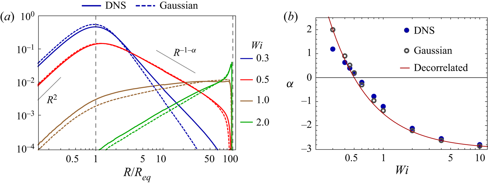
Figure 2. Stationary p.d.f.s of the end-to-end extension  $R$ of polymers in turbulent and random flows. (a) Comparison of the stationary p.d.f. of $R$, for different values of $\mathit {Wi}$, in DNS of turbulent flow and a synthetic Gaussian flow, constructed with the same Lyapunov exponent $\lambda$ as the DNS, as well as the same Lagrangian correlation times for vorticity $\tau _\varOmega$ and strain rate $\tau _S$. (b) The power-law exponent of the tail of the p.d.f. of $R$ in (a) presented as a function of $\mathit {Wi}$. The exponents from DNS are compared with that from the Gaussian flow, as well as with the prediction for a three-dimensional time-decorrelated random flow in (3.5).
Consider first the effect of the non-Gaussian statistics of turbulence. Figure 2(b) shows that low- $\mathit {Wi}$ stiff polymers stretch more in a turbulent flow than in a Gaussian flow: the values of $\alpha$ are less negative in the turbulent flow (compare the filled and open markers), which implies a greater power-law exponent for $p(R)$. Therefore, encountering a higher frequency of extreme-valued velocity gradients aids in stretching stiff polymers. Surprisingly, this is no longer true when $\mathit {Wi}$ is increased beyond $\mathit {Wi}_{cr}$. Rather, these moderately high- $\mathit {Wi}$ polymers, which are relatively easy to stretch, are seen to be more extended in a Gaussian flow than in a turbulent flow. On further increasing $\mathit {Wi}$, all three flows in figure 2(b) eventually exhibit nearly identical values of $\alpha$; this is to be expected since $\alpha$ must attain the limiting value $-3$ regardless of flow statistics (see § 3.1).
Why are moderately high- $\mathit {Wi}$ polymers stretched more in a Gaussian flow? To answer this, it is helpful to examine the p.d.f. of the rate of strain $s = \sqrt {S_{ij} S_{ij}}$ sampled by polymers. Figure 3(a) compares the distributions of $s$ for the turbulent and Gaussian flows. We see that the Gaussian flow has a comparative abundance of mild strain rate events to compensate for its lack of extreme-valued events. This suggests that high- $\mathit {Wi}$ polymers that have long relaxation times are stretched more effectively by mild persistent straining rather than by strong but short-lived straining. In contrast, stretching small- $\mathit {Wi}$ polymers that have short relaxation times requires strong strain rate events. These observations are consistent with a previous result by Terrapon et al. (Reference Terrapon, Dubief, Moin, Shaqfeh and Lele2004) for a turbulent channel flow. It was shown that stretching events at low $\mathit {Wi}$ are typically preceded by a burst of the strain rate; such bursts were not seen before stretching events at high $\mathit {Wi}$.

Figure 3. Effect of non-Gaussian velocity gradient fluctuations on polymer stretching in turbulence. (a) Comparison of the p.d.f. of the strain rate sampled by polymers in DNS of turbulent flow with that in a synthetic Gaussian flow with same  $\lambda$, $\tau _\varOmega$, $\tau _S$ as the DNS. The inset is a zoom that shows the near-peak behaviour of the distributions. (b) Illustration of the typical stretching dynamics of a $\mathit {Wi} = 0.8$ polymer in the DNS (upper plot) and Gaussian flows (lower plot). The grey shading shows when the polymer is stretched beyond a threshold $\ell = R_m/2=50$; each such time interval yields a value of $t_{str}$. (c) Distributions of $t_{str}$ for various values of $\mathit {Wi}$ in both DNS and Gaussian flows. The exponential tails of these p.d.f.s are associated with the time scale $T_{str}$. (d) Variation of $T_{str}$, the typical time spent by polymers in a stretched state, as a function of $\mathit {Wi}$, for both DNS and Gaussian flows. High- $\mathit {Wi}$ polymers in the Gaussian flow are seen to persist in a stretched state for significantly longer than they do in the DNS.
If it is true that high- $\mathit {Wi}$ polymers are stretched primarily by mild persistent straining, then they should not only stretch more in a Gaussian flow but also remain in an extended configuration for a longer duration of time. To detect this behaviour, we carry out a persistence time analysis and compare quantitatively how long polymers stay stretched in the turbulent and Gaussian random flows. Interestingly, the concept of persistence, which arose out of problems in non-equilibrium statistical physics (Majumdar Reference Majumdar1999; Bray, Majumdar & Schehr Reference Bray, Majumdar and Schehr2013), has been used recently to study the turbulent transport of particles and filaments (Kadoch et al. Reference Kadoch, del Castillo-Negrete, Bos and Schneider2011; Perlekar et al. Reference Perlekar, Ray, Mitra and Pandit2011; Bhatnagar et al. Reference Bhatnagar, Gupta, Mitra, Pandit and Perlekar2016; Singh, Picardo & Ray Reference Singh, Picardo and Ray2022).
We begin by defining a polymer to be in a ‘stretched’ state if  $R>\ell$, where the threshold $\ell = R_m/2$ is set well within the power-law range. The non-stretched state is then defined as $R \le \ell$. We have verified that varying the value of $\ell$ within the power-law range does not change our conclusions. With these states defined, we examine the Lagrangian history of each polymer, and detect the time intervals $t_{str}$ over which the polymer remains in a stretched state (see figure 3b). The distribution of this persistence time $p(t_{str})$ is presented in figure 3(c) for various $\mathit {Wi}$ and for both the turbulent and Gaussian flows. At large $t_{str}$, the distribution displays an exponential tail, $p(t_{str}) \sim \exp (-t_{str}/T_{str})$, from which we extract the persistence time scale $T_{str}$.
Figure 3(d) presents  $T_\mathrm {str}$ for both flows and for various values of $\mathit {Wi}$. Clearly, polymers with $\mathit {Wi} > \mathit {Wi}_{cr}$ typically remain stretched for a significantly longer time in the Gaussian flow as compared to the turbulent flow. This is true even for very large $\mathit {Wi}$ for which the exponent of the power law of $p(R)$ is nearly the same in both flows (see the results for $\mathit {Wi} \ge 2$ in figures 2b and 3d). So though the probability of large extensions is the same, the nature of stretching is different: polymers experience many short-lived episodes of large extension in the turbulent flow, whereas such episodes are fewer but last longer in the Gaussian flow.
Our study in this section of the differences between polymer stretching in turbulent and Gaussian flows has led to interesting physical insights; however, it is important to recognize that these differences are rather minor. Indeed, the Gaussian flow seems to provide a remarkably good approximation to a turbulent flow for studying polymer stretching statistics. Further support for this conclusion is provided in § 4.3, where we compare the evolution of the p.d.f. of  $R$ in the two flows, and in § 5, where we extend our study to the stretching of multi-bead chains.
Given that the p.d.f. and the Lagrangian temporal correlations (persistence) of  $R$ are unable to distinguish between the Gaussian and turbulent flows – the results are qualitatively alike – it is natural to ask whether Eulerian spatial correlations of polymer extension would be able to do so. First, consider polymers with small to moderate values of $\mathit {Wi}$. Their relatively rapid elastic relaxation implies that they will stretch only near regions of the flow with large strain rates. In turbulence, intense straining is localized in sheets that wrap around vortex tubes – a markedly different spatial organization compared with the random distribution expected for a Gaussian flow. Therefore, one should be able to tell the two flows apart by examining the spatial distribution of the most stretched polymers. However, as $\mathit {Wi}$ is increased to large values, the correlation between the extension of a polymer and the instantaneous strain rate will weaken. Once stretched, a high- $\mathit {Wi}$ polymer will remain extended over long intervals of time, even as it is advected across regions of the flow with varying strain rates.
The chaotic nature of turbulent advection will, at high  $\mathit {Wi}$, produce large gradients in the Eulerian field of polymer extension, $\hat {R}({\boldsymbol {x}})$. Such a field may be constructed from Lagrangian simulations by averaging over the extension of polymers in a given neighbourhood of $\boldsymbol {x}$, whereas in a continuum simulation (using e.g. the FENE-P model), $\hat {R}$ would be given by the square root of the trace of the conformation tensor. In the continuum context, the development of large gradients in $\hat {R}(\boldsymbol {x})$ leads to numerical instabilities – the high- $\mathit {Wi}$ problem – and special techniques are needed to simulate the field equations (Alves, Oliveira & Pinho Reference Alves, Oliveira and Pinho2021). Returning to our question, will these large gradients be produced in both the turbulent and Gaussian flows? We expect so. Recall indeed that when a passive scalar is mixed, the spatial concentration is highly intermittent with steep ramp–cliff structures, regardless of whether the carrier flow is Gaussian or turbulent (Shraiman & Siggia Reference Shraiman and Siggia2000; Falkovich et al. Reference Falkovich, Gawȩdki and Vergassola2001; Tsinober Reference Tsinober2009; Iyer et al. Reference Iyer, Schumacher, Sreenivasan and Yeung2018).
The above discussion of spatial correlations is limited to passive polymers. When feedback forces are present, the spatial correlations of the polymer extension field become closely coupled to those of the flow. At high  $\mathit {Wi}$, this coupling results in the emergence of an elastic scaling range in the kinetic energy spectrum, accompanied by a corresponding power-law range in the spatial spectrum of polymer energy or $\hat {R}^2$ (Fouxon & Lebedev Reference Fouxon and Lebedev2003; Steinberg Reference Steinberg2019). While there is some disagreement on the precise values of the scaling exponents, the presence of this new scaling range (above the dissipation scale and below the Kolmogorov inertial range) has been reported by several studies, both numerical (Nguyen et al. Reference Nguyen, Delache, Simoëns, Bos and El Hajem2016; Valente, da Silva & Pinho Reference Valente, da Silva and Pinho2016; Rosti et al. Reference Rosti, Perlekar and Mitra2023) and experimental (Vonlanthen & Monkewitz Reference Vonlanthen and Monkewitz2013; Zhang et al. Reference Zhang, Bodenschatz, Xu and Xi2021). Within this elastic range, the flow has been shown to be intermittent (Zhang et al. Reference Zhang, Bodenschatz, Xu and Xi2021; Rosti et al. Reference Rosti, Perlekar and Mitra2023) – the velocity structure functions scale anomalously – but the high-order structure functions of the polymer extension field have not been investigated yet. Future work in this direction would be helpful in understanding how extreme events arise and co-evolve in the face of strong fluid–polymer coupling.
4. Temporal evolution of the distribution of polymer extensions
4.1. Two regimes of evolution
Thus far, we have been studying the stationary p.d.f. of  $R$, attained after the polymers have spent enough time in the flow for their statistics to equilibrate. We now examine how the p.d.f. of $R$ evolves with time. Past work has shown that the p.d.f. relaxes exponentially to its stationary form, with a $\mathit {Wi}$-dependent time scale that exhibits a pronounced maximum at the coil–stretch transition (Celani et al. Reference Celani, Puliafito and Vincenzi2006; Watanabe & Gotoh Reference Watanabe and Gotoh2010). But what is the shape of the p.d.f. as it evolves? And how, if at all, does this evolution depend on $\mathit {Wi}$?
To answer these questions, we use our Lagrangian simulations to construct the p.d.f. of  $R$ as a function of time, $p(R,t)$. We consider an initial state in which the polymers are in equilibrium with a static fluid. So we first evolve the polymers with $\boldsymbol {\kappa } = 0$ (in (2.1)) until the p.d.f. of $R$ attains the equilibrium distribution (Bird et al. Reference Bird, Curtiss, Armstrong and Hassager1987). We then ‘turn on’ the turbulent flow.
The evolution of  $p(R,t)$ in the turbulent carrier flow is illustrated in figure 4. Interestingly, we find two qualitatively distinct regimes. At small or moderate $\mathit {Wi}$ (figure 4a), the p.d.f. is seen to quickly attain a power-law form with an exponent $\beta (t)$ that increases in time until it reaches its stationary value $\beta _\infty = -1-\alpha$. By fitting the distributions with a power law in the range $R_{eq} \ll R \ll R_m$, we find that $\beta (t)$ relaxes exponentially, i.e. $\beta _\infty -\beta \sim \exp (-t/T_\beta )$, as demonstrated in figure 4(b). The time scale $T_\beta$ is analysed in § 4.3.

Figure 4. Two regimes of evolution of the p.d.f. of the polymer extension. (a) Depiction of the evolving-power-law regime, seen for small to moderate  $\mathit {Wi}$, in which the tail of $p(R,t)$ evolves as $R^{\beta (t)}$. The thick black line with the time stamp $\lambda t = \infty$ represents the stationary p.d.f. of $R$. (b) The power-law exponent $\beta (t)$ is seen to approach its steady-state value $\beta _\infty = -1-\alpha$ exponentially. Here, $t_0$ is a reference time. (c,d) Depiction of the high- $\mathit {Wi}$ rapid-stretching regime, in which $p(R,t)$ does not evolve as a power law; rather, the p.d.f. quickly forms a local maximum near to $R_m$ (c), and then adjusts its shape directly to that of the stationary power law (d). These results are for the turbulent carrier flow.
The evolution at high  $\mathit {Wi}$ is quite different and is shown in figures 4(c,d). Here, the polymers stretch rapidly and quickly produce a local peak close to the maximum extension $R_m$. Thus although a transient power law appears at very early times, it is quickly lost as the local peak at $R_m$ begins to dominate the distribution (figure 4c). The long-time equilibration of the p.d.f. occurs by the peak near $R_m$ first approaching its stationary value; then the stationary power law $R^{\beta _\infty }$ gradually emerges, starting near $R_m$ and then extending its range down-scale towards $R_{{eq}}$ (figure 4d).
These two regimes of equilibration are termed the evolving-power-law regime and the rapid-stretching regime. The former occurs for  $\mathit {Wi} \lesssim 3/4$, while the latter occurs for larger $\mathit {Wi}$. Note that the crossover point, $\mathit {Wi} = 3/4$, is marked by a stationary p.d.f. with $\beta _\infty = 0$ that has neither a decaying tail at large $R$ nor a local peak near $R_m$; the evolution near $\mathit {Wi} = 3/4$ is a blend of the two regimes.
Does  $p(R,t)$ evolve in a similar fashion in the Gaussian flow? Yes, and we find the same two regimes of evolution, as illustrated in figure 5. The rates of relaxation, though, are different in the two flows. A quantitative comparison of the equilibration time scales is presented in § 4.3.

Figure 5. Comparison of the evolution of the p.d.f. of the polymer extension in the turbulent flow (solid lines) and the Gaussian flow (dashed lines), for (a) the evolving-power-law regime, and (b) the rapid-stretching regime.
4.2. The time-dependent power law: insights from a stochastic model
We now lend credence to the above characterization of the evolving-power-law regime by using a stochastic model to show that for  $0\leq \mathit {Wi}\lesssim 3/4$, an evolving power law is a natural consequence of scale separation between $R_{{eq}}$ and $R_m$. The associated analysis also reveals the $\mathit {Wi}$ dependence of the relaxation time scale $T_\beta$.
We consider the Batchelor–Kraichnan flow wherein the velocity gradient  $\boldsymbol {\kappa }(t)$ is a statistically isotropic, time-decorrelated, $3\times 3$ Gaussian tensor (Falkovich et al. Reference Falkovich, Gawȩdki and Vergassola2001). In terms of the scaled variables $r = R/R_{{eq}}$ and $\tilde {t}=t/2\tau$, the p.d.f. of the extension $p(r,\tilde {t})$ is governed by a Fokker–Planck equation (Martins Afonso & Vincenzi Reference Martins Afonso and Vincenzi2005; Plan, Ali & Vincenzi Reference Plan, Ali and Vincenzi2016)
 \begin{equation} \partial_{\tilde{t}} p={-}\partial_r[D_1(r)\,p]+\partial_r^2[D_2(r)\,p], \end{equation}
where
 \begin{equation} D_1(r)=[8\,\mathit{Wi}/3-f(r)]r+2/(3r), \quad D_2(r)=2\,\mathit{Wi}\, r^2/3+1/3, \end{equation}
and  $f(r)=1/(1-r^2/r_m^2)$. Note that while (4.1) is exact for the Batchelor–Kraichnan flow, an equation of the same form may be obtained for general turbulent flows by considering the Fokker–Planck equation associated with (2.1), assuming statistical isotropy, and modelling the stretching term à la Richardson, i.e. as a diffusive process. The associated extension-dependent eddy diffusivity should scale as $R^2$ since the extension remains below the viscous scale.
We assume a wide separation between the scales of the equilibrium and maximum extensions, i.e.  $R_m \gg R_{{eq}}$, or $r_m \gg 1$. Further, we focus on the long-time evolution of $p(r,\tilde {t})$, which is characterized by distinct behaviours for small, intermediate and very large extensions. (i) In the range of extensions where thermal fluctuations dominate ( $r<1$), the p.d.f. of $r$ assumes a quadratic profile (figure 2). (ii) For intermediate extensions, $1\ll r\ll r_m$, a power-law solution $r^{\beta (\tilde {t})}$ forms with an exponent $\beta (\tilde {t})$ that converges to its stationary value $\beta _\infty$. (iii) For extreme extensions, $p(r,\tilde {t})$ decreases rapidly as $r$ approaches $r_m$. We therefore introduce the ansatz

Here,  $\gamma$ is a threshold value of $r/r_m$, less than unity, beyond which the nonlinear part of the FENE spring coefficient $f(r)$ becomes non-negligible and terminates the power-law behaviour. The function $g(r,\tilde {t})$ is such that for $r = \gamma r_m$, we have $g(\gamma r_m,\tilde {t})=c(\tilde {t})\,(\gamma r_m)^{\beta (\tilde {t})}$, while for $r > \gamma r_m$, $g(r,\tilde {t})$ decreases faster than $r^{\beta (\tilde {t})}$ as $r$ approaches $r_m$. The latter assumption applies only if $\mathit {Wi} < 3/4$, for which $\beta _\infty < 0$. For larger $\mathit {Wi}$, our Lagrangian simulations show that the p.d.f. of $r$ develops a pronounced time-dependent peak between $\gamma r_m$ and $r_m$ (see figures 4c,d). Thus the subsequent analysis applies only for $\mathit {Wi} < 3/4$, which in fact corresponds to the regime in which the Lagrangian simulations exhibit an evolving power law.
The coefficient  $c(\tilde {t})$ is determined in terms of the exponent $\beta (\tilde {t})$ through the normalization condition

Clearly,  $I_1 = c/3$, while $I_2 = c[(\gamma r_m)^{1+\beta }-1]/[1+\beta ]$ for $\beta \neq -1$, and $I_2 = c \ln (\gamma r_m)$ for $\beta =-1$. For $r_m \gg 1$, $I_3$ is subdominant with respect to $I_1$ and $I_2$, and will be ignored. Thus solving (
) for  $c$ yields
 \begin{gather} c = \frac{1+\beta}{(\gamma r_m)^{1+\beta} + (\beta-2)/3} \quad \text{for $\beta \neq{-}1$}, \end{gather}
 \begin{gather}c = \frac{1}{1/3 +\ln(\gamma r_m)} \quad \text{for $\beta ={-}1$}. \end{gather}
To calculate  $\beta (\tilde {t})$, we observe that for $1 \ll r \ll r_m$, (4.1) can be simplified as
 \begin{equation} \partial_{\,\tilde{t}} p={-}\partial_r[(\tfrac{8}{3}\,\mathit{Wi}-1 ) r p]+\partial_r^2(\tfrac{2}{3}\,\mathit{Wi} \,r^2 p). \end{equation}
At steady state, we know that  $p(r) \propto r^{\beta _\infty }$, which when substituted into (4.6) yields $\beta _\infty =2 -3/(2\,\mathit {Wi})$, in accordance with the large deviations theory for a time-decorrelated flow (see (3.5) and recall that $\beta _\infty = -1-\alpha$).
Now, substituting  $p$ from (4.3b) into (4.6) results in
 \begin{equation} \left(\frac{\mathrm{d}c}{\mathrm{d} \beta}+c\ln r\right) \frac{\mathrm{d}\beta}{\mathrm{d}\tilde{t}}=c\,F(\beta,\mathit{Wi}), \end{equation}
with
 \begin{equation} F(\beta,\mathit{Wi})={-}(\tfrac{8}{3}\,\mathit{Wi}-1 )(1+\beta)+\tfrac{2}{3}\,\mathit{Wi}(1+\beta)(2+\beta). \end{equation}
The left-hand side of (4.7) contains  $\mathrm {d}c/{\mathrm {d} \beta }$, which is evaluated using (4.5):
 \begin{gather} \frac{\mathrm{d}c}{\mathrm{d} \beta} = c\left[\frac{1}{1+\beta}-\frac{(\gamma r_m)^{1+\beta} \ln{(\gamma r_m)}+1/3} {(\gamma r_m)^{1+\beta} +(\beta-2)/3}\right] \quad \text{for $\beta \neq{-}1$}, \end{gather}
 \begin{gather}\frac{\mathrm{d}c}{\mathrm{d} \beta} =0 \quad \text{for $\beta ={-}1$}. \end{gather}
On taking the limit  $r_m \gg 1$, the right-hand side of (4.9a) simplifies to $-3c/(\beta ^2-\beta -2)$ for $\beta < -1$, and to $-c\ln {(\gamma r_m)}$ for $\beta > -1$. By substituting these expressions for $\mathrm {d}c/{\mathrm {d} \beta }$ in (4.7) and considering that $r_m \gg r\gg 1$, we obtain the following leading-order equations for $\beta$:
 \begin{gather} \ln(r)\, \frac{\mathrm{d}\beta}{\mathrm{d}\tilde{t}}= F(\beta,\mathit{Wi}) \quad \text{for $\beta \leq{-}1$}, \end{gather}
 \begin{gather}\ln(\gamma r_m)\, \frac{\mathrm{d}\beta}{\mathrm{d}\tilde{t}}={-}F(\beta,\mathit{Wi}) \quad \text{for $\beta >{-}1$}. \end{gather}
Because  $\ln {(x)}$ is a weak function of $x$ for $x\gg 1$, we approximate $\ln r$ in (4.10a), as well as $\ln (\gamma r_m)$ in (4.10b), as $\ln r_m$ to obtain
 \begin{equation} \frac{\mathrm{d}\beta}{\mathrm{d}\tilde{t}} \approx a\, \frac{F(\beta,\mathit{Wi})}{\ln r_m}, \end{equation}
with  $a = 1$ for $\beta \leq -1$, and $a=-1$ for $\beta > -1$.
Being independent of  $r$, (4.11) shows that $p(R,t)$ may be approximated (up to logarithmic corrections) by a time-dependent power law in the range $R_{{eq}} \ll R \ll R_m$.
Next, to reveal the long-time relaxation of  $\beta$ to $\beta _\infty$, we substitute $\beta = \beta _{\infty }+ \beta '$ in (4.11) and linearize for small $\beta '$. Noting that $F(\beta _{\infty },\mathit {Wi}) = 0$ and that $\beta _{\infty } < -1$ for $\mathit {Wi} < \mathit {Wi}_{cr}$, we obtain
 \begin{gather} \frac{\mathrm{d}\beta'}{\mathrm{d}\tilde{t}} ={-}\frac{2 \left({\mathit{Wi}_{cr}-\mathit{Wi}}\right)}{\ln r_m}\,\beta' \quad {\rm for}\ \mathit{Wi} < \mathit{Wi}_{cr}, \end{gather}
 \begin{gather}\frac{\mathrm{d}\beta'}{\mathrm{d}\tilde{t}} ={-}\frac{2 \left({\mathit{Wi}-\mathit{Wi}_{cr}}\right)}{\ln r_m}\,\beta' \quad {\rm for}\ \mathit{Wi}_{cr} < \mathit{Wi} < 3/4. \end{gather}
In terms of dimensional time  $t$, this implies an exponential relaxation of the power-law exponent,
 \begin{equation} \beta_{\infty} - \beta(t) \sim \exp({-}t/T_\beta), \end{equation}
with a time scale
 \begin{equation} T_\beta \sim \frac{\tau}{|\mathit{Wi}-\mathit{Wi}_{cr}|} \end{equation}
that diverges as  $\mathit {Wi}$ approaches $\mathit {Wi}_{cr}$.
Note that (4.11) actually has two fixed points:  $\beta _\infty$ and $-1$. The latter, though, can be shown to be dynamically unstable, leaving $\beta _\infty$ as the only stable fixed point.
The prediction (4.13) of an exponentially relaxing power-law exponent is certainly in agreement with the results of our Lagrangian simulations (see figure 4b). The  $\mathit {Wi}$ dependence of the relaxation time scale will be examined in light of (4.14) in the next section. But first, it is instructive to compare (4.13)–(4.14) against numerical simulations of the Fokker–Planck equation (4.1). Beginning from a distribution of coiled dumbbells, we solve (4.1) using second-order central differences and the LSODA algorithm (Petzold Reference Petzold1983) with adaptive time stepping (Wolfram Research 2019). We take $R_m = 10^3 R_{{eq}}$, thereby realizing a much larger scale separation than is practical in our Lagrangian simulations. The results are presented in figure 6.

Figure 6. Evolution of the p.d.f. of the extension as predicted by numerical simulations of the Fokker–Planck equation for the Batchelor–Kraichnan flow (with  $R_m = 10^3 R_{{eq}}$): (a) the evolving-power-law regime, (b) the rapid-stretching regime. (c) The time scale of relaxation $T_\beta$ of the evolving power-law exponent is shown as a function of $\mathit {Wi}$. The dashed line shows the variation predicted by the asymptotic analysis (cf. (4.13)).
The stochastic model exhibits the same two regimes of evolution as the Lagrangian simulations: the evolving-power-law regimes for  $\mathit {Wi} < 3/4$ (cf. figures 4a and 6a) and the rapid-stretching regime for larger $\mathit {Wi}$ (cf. figures 4c,d and 6b). Within the evolving-power-law regime, we extract the exponent $\beta (t)$ and find that it does in fact evolve exponentially, in accordance with (4.13). The time scale $T_\beta$, obtained from a least squares fit, is presented as a function of $\mathit {Wi}$ in figure 6(c). The predicted divergence of $T_\beta$ at $\mathit {Wi}_{cr}$ (see (4.14)) manifests in the simulations (which have a finite scale separation) as a prominent maximum of $T_\beta$ at $\mathit {Wi}_{cr}$. Such a slowing down of the stretching dynamics at the coil–stretch transition was demonstrated by Martins Afonso & Vincenzi (Reference Martins Afonso and Vincenzi2005) and Celani et al. (Reference Celani, Puliafito and Vincenzi2006), but in regard to the equilibration of the entire p.d.f. of $R$. The behaviour of $T_\beta$ versus $\mathit {Wi}$ gives an alternative characterization of the same phenomenon.
4.3. Time scales of equilibration of  $p(R,t)$ in random and turbulent flows

We now compare quantitatively the time scales of equilibration of  $p(R,t)$ in the turbulent and Gaussian flows (Lagrangian simulations) as well as in the Batchelor–Kraichnan decorrelated flow (numerical solution of the stochastic model).
One time scale of interest is that associated with the evolving power-law tail,  $T_\beta$. However, this time scale is relevant only for $\mathit {Wi} < 3/4$. So, to characterize the equilibration time for all $\mathit {Wi}$, we use the time scale associated with the entire p.d.f. of $R$. Martins Afonso & Vincenzi (Reference Martins Afonso and Vincenzi2005) and Celani et al. (Reference Celani, Puliafito and Vincenzi2006) showed, for random flows, that $p(R,t)$ approaches its asymptotic stationary form exponentially, with a time scale $T_P$ that displays a maximum near $\mathit {Wi}_{cr}$. Watanabe & Gotoh (Reference Watanabe and Gotoh2010) confirmed this prediction in DNS of isotropic turbulence. We obtain $T_P$ from our simulations by fitting the evolution of the first moment of $p(R,t)$ (approximately the same value is obtained by fitting the higher moments).
Figures 7(a,b) present the equilibration time scales  $T_\beta$ and $T_P$, respectively, for the turbulent flow (filled markers) and the Gaussian flow (open markers). The results for the time-decorrelated Batchelor–Kraichnan flow are also presented (line). We see that the qualitative variation of these time scales with $\mathit {Wi}$ is the same in all flows and exhibits a maximum near $\mathit {Wi}_{cr}$. In the case of $T_P$, a $\mathit {Wi}^{-1}$ asymptotic behaviour is visible (see the inset of figure 7b), in agreement with Martins Afonso & Vincenzi (Reference Martins Afonso and Vincenzi2005) and Celani et al. (Reference Celani, Puliafito and Vincenzi2006).

Figure 7. Effect of non-Gaussian velocity gradient statistics on the time scale of evolution of the p.d.f. of the extension to its stationary form. (a) Comparison of the relaxation time scale  $T_\beta$ of the power-law exponent of the tail of the p.d.f. of $R$ obtained from DNS (cf. figure 4b) with that from the synthetic Gaussian flow as well as the Batchelor–Kraichnan flow (simulations of (4.1)). (b) Comparison of the exponential relaxation time scale $T_P$ of the entire p.d.f. of $R$, for the three different cases: DNS, Gaussian flow and Batchelor–Kraichnan flow. The inset is a log-log plot of the same data that shows the $\mathit {Wi}^{-1}$ asymptotic behaviour.
On comparing the results for the turbulent and time-decorrelated flows, we see that the time correlation of the flow slows down the equilibration of the p.d.f. of  $R$: both $T_\beta$ and $T_P$ are higher for the turbulent flow (figures 7a,b) than for the decorrelated flow. Therefore, by incorporating temporal correlations, the Gaussian flow is able to provide a better approximation to the turbulent flow, though the time scales are still slightly higher in the turbulent flow for most values of $\mathit {Wi}$.
These results show that one can obtain a good first approximation of the stretching statistics of elastic dumbbells in turbulence by using a correlated Gaussian velocity gradient; this is true not only for stationary statistics, as seen in § 3.2, but also for temporally evolving statistics. Is this outcome specific to the simple FENE dumbbell? This question is addressed in the next section, where we find that the Gaussian flow remains a good approximation even for multi-bead chains.
This study has shown how the distribution of extensions  $p(R,t)$ evolves from an initial state in which the polymers are coiled and uniformly distributed in space. Alternately, the polymers may be localized initially, as when a concentrated polymer solution is injected into a turbulent bath of pure solvent. In the passive limit, the polymers will spread out like tracers. After an initial time, of the order of $\lambda ^{-1}$, the chaotic nature of the flow will ensure that the polymers forget their initial conditions. Moreover, since $\boldsymbol {\nabla } \boldsymbol {u}$ and $\boldsymbol {u}$ are weakly correlated in a turbulent flow (Pumir et al. Reference Pumir, Xu, Bodenschatz and Grauer2016), the stretching and advection of the polymers will proceed independently. So $p(R,t)$ will evolve – in the long term – in a manner similar to that described in this section; meanwhile, the blob of polymers will disperse, first à la Richardson (up to the large-eddy scale), and then in a diffusive manner (Davidson Reference Davidson2015).
The situation is altered considerably, however, when polymer feedback forces are significant. In one of the few studies involving an initially localized distribution of polymers, Vaithianathan et al. (Reference Vaithianathan, Rovert, Brasseur and Collins2007) have shown that elastic feedback forces locally suppress the small scales of the flow and thereby reduce the rate of dispersion. Therefore, the blob of polymers will spread more slowly in the presence of feedback forces. The mean strain rate within the blob will reduce as well, so  $p(R,t)$ will also evolve more slowly than in the passive case. However, as the blob disperses and entrains pure solvent, the concentration of polymers will decrease and the effects of feedback will weaken. In general, the coupled dynamics of flow and mixing in a non-uniform polymer solution are not well understood and warrant further detailed investigation.
5. Chains stretch like equivalent dumbbells
Thus far, we have focused on the simplest model for a polymer of finite extension, the FENE dumbbell (§ 2.1). We now show that the key results presented above also hold for a polymer chain, which incorporates higher-order deformation modes.
The three-dimensional motion of a freely-jointed (Rouse) chain, composed of  $\mathscr {N}$ beads, is described in terms of the position of its centre of mass $\boldsymbol {X}_c$ and the separation vectors between the beads $\boldsymbol {Q}_i$ ( $i=1,\dots,\mathscr {N}-1$) (Bird et al. Reference Bird, Curtiss, Armstrong and Hassager1987; Öttinger Reference Öttinger1996):
 \begin{gather} \dot{\boldsymbol{X}}_c = \boldsymbol{u}(\boldsymbol{X}_c(t),t)+\dfrac{1}{\mathscr{N}}\,\sqrt{\frac{Q_{{eq}}^2}{6\tau_*}}\, \sum_{i=1}^{\mathscr{N}}\boldsymbol{\xi}_i(t),\end{gather}
 \begin{align} \dot{\boldsymbol{Q}_i} &=\boldsymbol{\kappa}(t)\boldsymbol{\cdot}\boldsymbol{Q}_i(t)-\dfrac{1}{4\tau_*}\, [2f_i\,\boldsymbol{Q}_i(t)-f_{i+1}\,\boldsymbol{Q}_{i+1}(t)-f_{i-1}\,\boldsymbol{Q}_{i-1}(t)]\nonumber\\ &\quad +\sqrt{\dfrac{Q_{{eq}}^2}{6\tau_*}}\, [\boldsymbol{\xi}_{i+1}(t)-\boldsymbol{\xi}_i(t)],\quad i=1,\dots,\mathscr{N}-1, \end{align}
 where each link is associated with an elastic time scale  $\tau _*$ and has an equilibrium r.m.s. extension $Q_{{eq}}=\sqrt {3k_BT/H}$. The FENE interactions between neighbouring beads are characterized by the coefficients
 \begin{equation} f_i=\dfrac{1}{1-\vert\boldsymbol{Q}_i\vert^2/Q_m^2}, \end{equation}
which ensure that the extension of each spring does not exceed its maximum length  $Q_m$. The Brownian forces that act on the beads are represented by independent, vectorial, white noises $\boldsymbol {\xi }_i(t)$. Note that one must set $\boldsymbol {Q}_0=\boldsymbol {Q}_{\mathscr {N}}=0$ in the equations for $\boldsymbol {Q}_1$ and $\boldsymbol {Q}_{\mathscr {N}-1}$.
The end-to-end separation or extension vector of the polymer chain is defined as  $\boldsymbol {R}=\sum _{i=1}^{\mathscr {N}-1}\boldsymbol {Q}_i$. In a still fluid, the equilibrium r.m.s. value of $\vert \boldsymbol {R}\vert$ is $Q_{{eq}}\sqrt {\mathscr {N}-1}$ (Bird et al. Reference Bird, Curtiss, Armstrong and Hassager1987).
In order to compare the extensional dynamics of a chain and a dumbbell, Jin & Collins (Reference Jin and Collins2007) proposed the following mapping between the parameters of the two models:
 \begin{equation} R_{{eq}} = Q_{{eq}}\sqrt{\mathscr{N}-1}, \quad R_m = Q_m\sqrt{\mathscr{N}-1}, \quad \tau = \frac{(\mathscr{N}+1)\mathscr{N}}{6}\,\tau_*. \end{equation}
This map is obtained by starting with the relation between  $R_{{eq}}$ and $Q_{{eq}}$, which follows from the random walk theory for a polymer in a still fluid (de Gennes Reference de Gennes1979), and then using it in an expression for the elongational viscosity of highly stretched polymers given by Wiest & Tanner (Reference Wiest and Tanner1989). By requiring the value of the viscosity thus obtained to be independent of $\mathscr {N}$, one obtains the relation between the time scale of the springs of an $\mathscr {N}$-bead chain, $\tau _*$, and that of an equivalent dumbbell, $\tau$ (Jin & Collins Reference Jin and Collins2007). This mapping was shown by Watanabe & Gotoh (Reference Watanabe and Gotoh2010) to work very well for the stationary p.d.f. of $R$ (see the inset of figure 8(d) for a comparison of the power-law exponent corresponding to the stationary p.d.f.). Here, we check to see if it works equally well for the temporal evolution of the distribution.

Figure 8. Effect of the polymer model – bead–spring dumbbell or chain – on the evolution of the p.d.f. of the extension in the turbulent carrier flow. (a) Comparison of the evolving p.d.f. of  $R$, in the evolving-power-law regime, of an $\mathscr {N}=10$ chain (solid line) with that of an equivalent dumbbell (dashed line). The parameters of the dumbbell are given by (5.3a–c). (b) Comparison of the evolution of the p.d.f. of $R$ in the rapid-stretching regime. (c) Comparison of the relaxation time $T_\beta$ of the power-law exponent of the evolving p.d.f. for the chain and dumbbell, and for various $\mathit {Wi}$ in the evolving-power-law regime. (d) Comparison of the exponential relaxation time scale $T_P$ of the entire p.d.f. of $R$ for the chain and the dumbbell. The inset compares the power-law exponents of the stationary p.d.f.s.
Figure 8 compares the evolution and equilibration of the p.d.f. of  $R$ for a dumbbell and an $\mathscr {N}=10$ chain, in the turbulent carrier flow. Figures 8(a,b) depict the evolution of $p(R,t)$ for a small and high $\mathit {Wi}$, respectively. The results agree quite well in both cases. Figure 8(c) compares the equilibration time scale of the evolving power law, $T_\beta$, while figure 8(d) compares the equilibration time scale of the entire p.d.f., $T_P$. While the results for the dumbbell and chain are similar for all $\mathit {Wi}$, they are in excellent agreement at high $\mathit {Wi}$. This is unsurprising, given that the mapping (5.3a–c) was derived by equating the elongation viscosity of highly stretched chains and dumbbells (Jin & Collins Reference Jin and Collins2007).
We have seen, in §§ 3.2 and 4.3, that the Gaussian flow is a rather good surrogate for the turbulent flow, with regard to the stretching statistics of dumbbells. We now check whether this is true for the stretching of chains as well. Figure 9(a) compares the power-law exponent  $\alpha$ of the stationary p.d.f. of $R$ for 10-bead chains in the two flows. The analytical prediction for a dumbbell in a time-decorrelated flow – the simplest possible combination of a chaotic flow and a polymer model – is also shown for comparison. As in the case of dumbbells (figure 2b), we see that the stretching of chains is stronger in the turbulent flow, at low $\mathit {Wi}$, while it is slightly stronger in the Gaussian flow, at moderately high $\mathit {Wi}$. Figure 9(b) compares the evolution of the p.d.f. of $R$ via the equilibration time scale $T_P$; the results for the two flows agree rather well, just as they do for dumbbells (figure 7b). A similar agreement is found for the values of $T_\beta$ in the two flows (not shown). Thus we may conclude that, apart from small quantitative differences, a correlated Gaussian flow provides a good approximation to a turbulent flow for studying the stretching statistics of polymers.
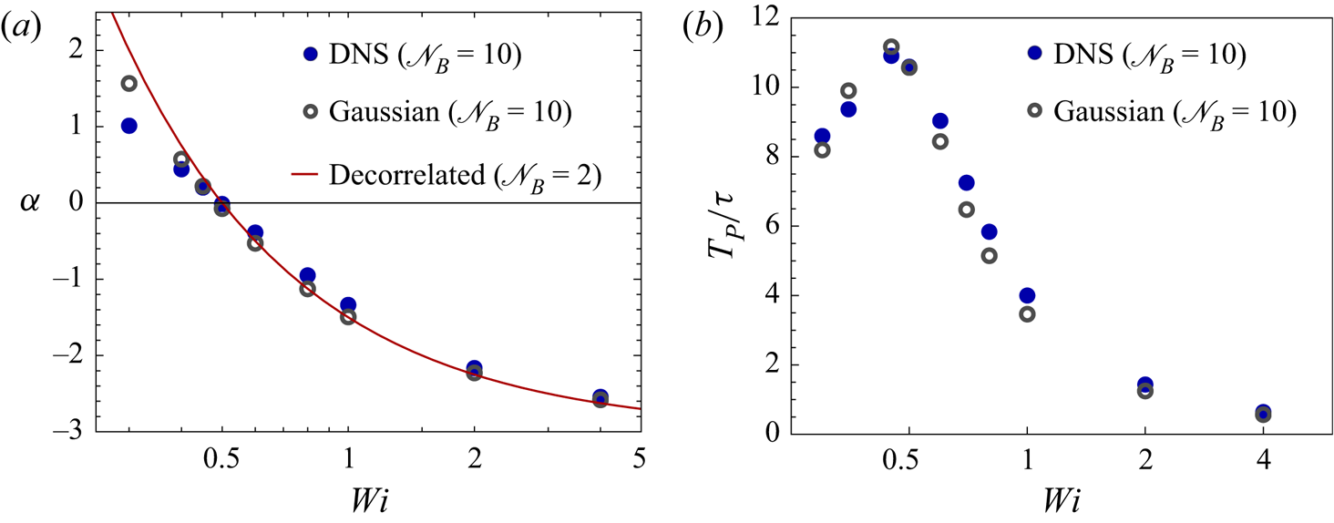
Figure 9. Comparison of the stretching statistics of 10-bead chains in turbulent and Gaussian flows. (a) Comparison of the exponent  $\alpha$ of the power-law tail of the stationary p.d.f. of $R$, for different values of $\mathit {Wi}$. (b) Comparison of the exponential time scale $T_P$ with which the p.d.f. of $R$ relaxes to its stationary form. These two plots are similar to those corresponding to dumbbells, namely figures 2(b) and 7(b), respectively.
6. Concluding remarks
Polymers in a chaotic flow field stretch and coil repeatedly, sampling a broad distribution of extensions. The basic features of the stationary distribution – a power-law tail and the coil–stretch transition – are well documented and understood in terms of the large deviations theory. In this work, we have examined the stretching dynamics in more detail to understand how the stationary distribution of extensions is attained, and how polymers respond to the non-Gaussian time-correlated velocity gradient statistics of turbulence.
We have seen that extreme strain rates are important only for stretching stiff low- $\mathit {Wi}$ polymers, whereas it is mild but persistent straining that extends more elastic high- $\mathit {Wi}$ polymers. This insight has relevance for the extension of polymers in the presence of two-way coupling with the flow. The feedback forces exerted by polymers onto the flow not only reduce the mean value of the strain rate but also suppress its extreme-valued fluctuations (Perlekar et al. Reference Perlekar, Mitra and Pandit2010; ur Rehman et al. Reference ur Rehman, Lee and Lee2022). Clearly, the reduction in the mean strain rate will cause two-way coupled polymers to stretch less, on average, than one-way coupled passive polymers. In fact, at large values of $\mathit {Wi}$, this effect can be strong enough to cause the mean extension to decrease with increasing $\mathit {Wi}$ (Rosti et al. Reference Rosti, Perlekar and Mitra2023). But what if one compensates for the reduced mean value by suitable rescaling? Would we see a separate effect of the loss of extreme events, arising from just the change in the shape of the distribution of strain rates? This question was addressed in recent Eulerian–Lagrangian simulations by ur Rehman et al. (Reference ur Rehman, Lee and Lee2022). They defined an effective $\mathit {Wi}$ for two-way coupled polymers, using the reduced value of the Kolmogorov time scale of the modified flow, and then compared the stretching statistics of two-way and one-way coupled polymers. They found that the mean and standard deviation of the p.d.f. of extension are almost the same for one-way and two-way coupled polymers with the same effective $\mathit {Wi}$. This was despite the fact that the feedback forces were strong enough to substantially modify the net dissipation rate, as well as the statistics of vorticity and strain rate. This result is understandable, indeed is to be expected, in light of our results. At small $\mathit {Wi}$, where extreme strain rates are important, the feedback force and thus the modification of the flow will be weak; at large $\mathit {Wi}$, the extreme strain rates are no longer important for stretching and their loss does not impact the extent of stretching. It should be noted that the simulations of ur Rehman et al. (Reference ur Rehman, Lee and Lee2022) were carried out at a low volume fraction; the impact of feedback forces on polymer stretching may differ at larger volume fractions.
Examining the time evolution of the p.d.f. of extensions, we have identified two regimes: the low- $\mathit {Wi}$ evolving-power-law regime and the high- $\mathit {Wi}$ rapid-stretching regime. In both regimes, the p.d.f. equilibrates exponentially with a time scale that peaks near the coil–stretch transition. While performing experiments or simulations at low to moderate $\mathit {Wi}$, one should bear in mind that the non-stationary p.d.f. has the form of an evolving power law, so that the mere appearance of a power-law subrange is not construed as evidence for having attained stationarity.
A question that is closely related to the effect of extreme-valued strain rates is: how does the Reynolds number of the flow affect polymer stretching? The turbulent carrier flow used in our simulations has Taylor–Reynolds number  ${Re}_\lambda \approx 111$. Though modest, this value is sufficient for the strain rate to exhibit strongly non-Gaussian statistics (figure 3a), i.e. compared to a Gaussian distribution, the frequency of extreme strain rates is much larger, while that of mild strain rates is much smaller. This intermittent nature of the velocity gradient has been shown to produce more stretching of low- $\mathit {Wi}$ polymers but less stretching of moderately high- $\mathit {Wi}$ polymers (very-high- $\mathit {Wi}$ polymers are unaffected). So we expect that as ${Re}_\lambda$ increases, and the velocity gradient becomes more intermittent (Buaria et al. Reference Buaria, Pumir, Bodenschatz and Yeung2019), low- $\mathit {Wi}$ polymers will stretch more while moderately high- $\mathit {Wi}$ polymers will stretch less. We do not expect to see new features in the statistics, though, since the p.d.f. of polymer extensions exhibits the same qualitative behaviour in our turbulent flow as in the random Gaussian flow.
While most of this work has considered the FENE dumbbell, we have shown that our results are valid for a bead–spring chain as well. However, for simplicity we have neglected inter-bead hydrodynamics interactions (HI) and excluded volume (EV) forces. These forces do not play a role once polymers are stretched, but they do affect the time it takes for polymers to unravel (Schroeder et al. Reference Schroeder, Shaqfeh and Chu2004; Sim, Khomami & Sureshkumar Reference Sim, Khomami and Sureshkumar2007; Vincenzi et al. Reference Vincenzi, Watanabe, Ray and Picardo2021). Understanding their effect on individual polymer stretching and ultimately on the turbulent dynamics of polymer solutions is an important area for future work.
One of the challenges in developing accurate models for polymers that undergo rapid stretching in turbulence is the large computational cost involved in simulating complex polymer chains in a turbulent flow. This difficulty would be greatly reduced if the DNS for the flow are replaced by a stochastic model for the Lagrangian velocity gradient. The results of our study show that this would indeed be a useful strategy, because the stretching dynamics have been shown to be only mildly sensitive to the detailed statistics of the velocity gradient. For example, one could use the time-correlated Gaussian velocity gradient for testing the consequence of including forces like EV and HI, and for developing coarse-grained effective dumbbell models. The latter could then be used for Lagrangian simulations in DNS of turbulent polymer solutions.
In this work, we have intentionally used a Gaussian model for the velocity gradient, in order to study the influence of the extreme-valued statistics of the turbulent velocity gradient. To include non-Gaussian effects and obtain a more accurate prediction of polymer stretching, one could use stochastic models for the velocity gradient that are based on the restricted Euler equations (Vieillefosse Reference Vieillefosse1982), in turn derived from the Navier–Stokes equations (Meneveau Reference Meneveau2011). An early example is the model of Girimaji & Pope (Reference Girimaji and Pope1990), which produces stationary velocity gradient statistics with many realistic features, including non-Gaussianity. However, the model requires prior knowledge of the moments of the velocity gradient. A similar drawback is present in the Gaussian random model used in this work, which requires the temporal correlation of vorticity and strain, along with the Lyapunov exponent, to be specified as inputs. In contrast, the model of Chevillard & Meneveau (Reference Chevillard and Meneveau2006, Reference Chevillard and Meneveau2007), based on the recent fluid deformation approximation, has an input parameter that takes the place of the Reynolds number; once this parameter is specified, the model generates statistics with appropriate moments and temporal correlations. However, this model is restricted to moderate values of  ${Re}_\lambda$ (Meneveau Reference Meneveau2011). This limitation has been overcome by the multifractal model of Pereira, Moriconi & Chevillard (Reference Pereira, Moriconi and Chevillard2018), which produces realistic statistics of the velocity gradient for large values of ${Re}_\lambda$. It would be interesting to use such a model to study polymer stretching at very large ${Re}_\lambda$, and to check whether increasing ${Re}_\lambda$ has opposing effects on low- and high- $\mathit {Wi}$ polymers.
Acknowledgements
The authors are grateful to S.S. Ray for sharing his database of Lagrangian trajectories in homogeneous and isotropic turbulence. J.R.P. and D.V. acknowledge their Associateships with the International Centre for Theoretical Sciences (ICTS), Tata Institute of Fundamental Research, Bangalore, India. D.V. would like to thank the Isaac Newton Institute for Mathematical Sciences for support and hospitality during the programme ‘Mathematical aspects of turbulence: where do we stand?’ when work on this paper was undertaken. J.R.P. is similarly grateful for the hospitality provided by the ICTS, Bangalore. D.V. and J.R.P. also thank the OPAL infrastructure, the Center for High-Performance Computing of Université Côte d'Azur, and the ICTS, Bangalore, for computational resources. Simulations were also performed on the IIT Bombay workstations Aragorn and Gandalf (procured through grant SRG/2021/001185).
Funding
This work was supported by IRCC, IIT Bombay (J.R.P., seed grant), DST-SERB (J.R.P., grant no. SRG/2021/001185), Fédération de Recherche Wolfgang Doeblin (J.R.P.), the Agence Nationale de la Recherche (D.V., grant nos ANR-21-CE30-0040-01, ANR-15-IDEX-01), EPSRC (D.V., grant no. EP/R014604/1), the Simons Foundation (D.V.), the Indo–French Centre for Applied Mathematics IFCAM (J.R.P. and D.V.), and the Indo–French Centre for the Promotion of Advanced Scientific Research (IFCPAR / CEFIPRA) (J.R.P. and D.V., project no. 6704-A).
Declaration of interests
The authors report no conflict of interest.


 Open access