


1. Introduction
Hydrodynamic instabilities such as Rayleigh–Taylor (RT) instability and Richtmyer– Meshkov (RM) instability play an important role in natural and industrial fields such as astrophysics (Abarzhi et al. Reference Abarzhi, Bhowmick, Naveh, Pandian, Swisher, Stellingwerf and Arnett2019), supersonic combustion (Yang, Kubota & Zukoski Reference Yang, Kubota and Zukoski1993) and inertial confinement fusion (ICF) (Lindl et al. Reference Lindl, Landen, Edwards, Moses and Team2014). The RT instability (Rayleigh Reference Rayleigh1883; Taylor Reference Taylor1950) occurs when a perturbed interface separating two fluids of different densities is in a gravitational field (or an acceleration field) pointing from heavy fluid to light. The RM instability (Richtmyer Reference Richtmyer1960; Meshkov Reference Meshkov1969) occurs when a perturbed interface between two different fluids is subjected to an impulsive acceleration, typically by a shock wave. From the loading point of view, RM instability can be viewed as an impulsive variant of RT instability. Although the two instabilities share common evolution processes, such as the formation of spike (heavy fluid penetrates into light) and bubble (light fluid rises into heavy), and the flow transition to turbulent mixing (under a certain condition), their evolution regimes are distinct. This impedes the straightforward application or extension of the knowledge of RT instability to RM instability.
Over the past decades, much attention has been paid to RM instability, and substantial progress has been achieved in theory (Richtmyer Reference Richtmyer1960; Zhang & Sohn Reference Zhang and Sohn1997; Dimonte & Ramaprabhu Reference Dimonte and Ramaprabhu2010; Nishihara et al. Reference Nishihara, Wouchuk, Matsuoka, Ishizaki and Zhakhovsky2010; Zhang, Deng & Guo Reference Zhang, Deng and Guo2018), experiment (Prestridge et al. Reference Prestridge, Orlicz, Balasubramanian and Balakumar2013; Biamino et al. Reference Biamino, Jourdan, Mariani, Houas, Vandenboomgaerde and Souffland2015; Reese et al. Reference Reese, Ames, Noble, Oakley and Bonazza2018; Mohaghar et al. Reference Mohaghar, Carter, Pathikonda and Ranjan2019; Sewell et al. Reference Sewell, Ferguson, Krivets and Jacobs2021) and simulation (Schilling & Latini Reference Schilling and Latini2010; Lombardini, Pullin & Meiron Reference Lombardini, Pullin and Meiron2014; Wonga & Lelea Reference Wonga and Lelea2017; Groom & Thornber Reference Groom and Thornber2021; Li et al. Reference Li, Fu, Yu and Li2022b). The existing studies are concerned mainly with RM instability at a single interface. This is not the case for real situations, in which RM instability occurs usually at two or multiple interfaces. For example, an ICF capsule usually consists of three concentric shells – the outer ablator, the middle solid deuterium-tritium (DT) ice and the inner gaseous DT fuel – which form two material interfaces (Betti & Hurricane Reference Betti and Hurricane2016). As the capsule is irradiated by high-power X-rays (indirect drive) or laser beams (direct drive), shock waves are generated, which subsequently propagate inwards, triggering RM instability at both the inner and outer interfaces. Also, in a supernova explosion, the stellar collapse produces a strong divergent shock, which moves outwards and passes across the multi-layer elements, inducing RM instability (Arnett et al. Reference Arnett, Bahcall, Kirshner and Woosley1989). It is therefore more valuable practically to investigate RM instability at a finite-thickness fluid layer with two interfaces.
RM instability at an SF $_6$ layer embedded in air impacted by a planar shock wave was first realized by Jacobs et al. (Reference Jacobs, Klein, Jenkins and Benjamin1993) in a shock-tube experiment, and three distinct flow patterns – including the upstream mushroom, downstream mushroom and sinuous mode – were observed. The random emergence of three flow patterns in the experiment of Jacobs et al. (Reference Jacobs, Klein, Jenkins and Benjamin1993) was ascribed to the sensitivity of the layer evolution to its initial shape (Budzinski, Benjamin & Jacobs Reference Budzinski, Benjamin and Jacobs1994; Jacobs et al. Reference Jacobs, Jenkins, Klein and Benjamin1995). Also, Rightley et al. (Reference Rightley, Vorobieff, Martin and Benjamin1999) examined experimentally the evolution of a shock-accelerated gas layer with various initial perturbations, and an abrupt mixing transition was observed for a multi-mode initial perturbation. Since then, turbulent mixing developing from RM instability at a gas layer (called RM turbulence) has been investigated continually with laser-sheet imaging techniques such as particle image velocimetry and planar laser induced fluorescence. The effect of initial conditions (the layer shape, the concentration distribution, the shock strength, etc.) and the influence of reflected shock on the RM turbulence were analysed especially (Prestridge et al. Reference Prestridge, Rightley, Vorobieff, Benjamin and Kurnit2000; Balakumar et al. Reference Balakumar, Orlicz, Tomkins and Prestridge2008, Reference Balakumar, Orlicz, Ristorcelli, Balasubramanian, Prestridge and Tomkins2012; Tomkins et al. Reference Tomkins, Kumar, Orlicz and Prestridge2008; Orlicz et al. Reference Orlicz, Balakumar, Tomkins and Prestridge2009; Orlicz, Balasubramanian & Prestridge Reference Orlicz, Balasubramanian and Prestridge2013; Tomkins et al. Reference Tomkins, Balakumar, Orlicz, Prestridge and Ristorcelli2013). In all the above experiments, the gas layer is produced by vertically injecting a gas curtain into the test section of the shock tube through a contoured nozzle. Although the jet technique greatly facilitates the experimental study of RM instability, it brings several uncertainties into initial conditions, such as the non-uniform distribution of gas concentration inside the layer, initial velocity of the test gas in the vertical direction, three-dimensionality and gas diffusion, which could evidently influence the instability growth (Tomkins et al. Reference Tomkins, Kumar, Orlicz and Prestridge2008; Orlicz et al. Reference Orlicz, Balakumar, Tomkins and Prestridge2009; Bai et al. Reference Bai, Zou, Wang, Liu, Huang, Liu, Li, Tan and Liu2010; Balasubramanian, Orlicz & Prestridge Reference Balasubramanian, Orlicz and Prestridge2013; Shankar & Lele Reference Shankar and Lele2013).
Recently, a novel soap-film technique was developed to create a sharp gaseous interface with controllable shape (Liu et al. Reference Liu, Liang, Ding, Liu and Luo2018). A series of elaborate experiments demonstrated that this technique can largely eliminate three-dimensionality and gas diffusion. In addition, the soap film was found to produce a negligible influence on the interface evolution at early to intermediate stages (Liang et al. Reference Liang, Liu, Zhai, Ding, Si and Luo2021; Guo et al. Reference Guo, Cong, Si and Luo2022; Chen et al. Reference Chen, Xing, Wang, Zhai and Luo2023). More recently, this soap-film technique was extended to generate gas layers with controllable shape and thickness, which enables the experimental study on RM instability at various types of controllable gas layers (Liang & Luo Reference Liang and Luo2021a, Reference Liang and Luo2022). Experimental results showed that the reverberating waves inside the layer could induce RT instability/stability, which promotes/suppresses the instability growth. In addition, an interface coupling effect is evident (particularly for a thin layer), which significantly affects the instability growth at both interfaces of the layer (Jacobs et al. Reference Jacobs, Jenkins, Klein and Benjamin1995; Mikaelian Reference Mikaelian1995, Reference Mikaelian2005). The soap-film technique was also developed to generate gas layers in the test section of a semi-annular convergent shock tube, with which a series of experiments on convergent RM instability at a perturbed gas layer were realized (Ding et al. Reference Ding, Li, Sun, Zhai and Luo2019; Li et al. Reference Li, Ding, Si and Luo2020a, Reference Li, Ding, Luo and Zou2022a; Sun et al. Reference Sun, Ding, Zhai, Si and Luo2020). Convergent RM instability is more complex than the planar counterpart due to the existence of a geometric convergence effect and reshock (Bell Reference Bell1951; Plesset Reference Plesset1954; Epstein Reference Epstein2004). Also, the shocked interface is decelerated when it approaches the geometric centre, inducing RT instability/stability (Ding et al. Reference Ding, Si, Yang, Lu, Zhai and Luo2017b). These new regimes could couple with interface coupling and wave influence, providing more possibilities and complexities for the growth of convergent RM instability at a gas layer.
The existing studies were limited to RM instability induced by planar and convergent shocks. So far, RM instability at a gas layer induced by a divergent shock (i.e. divergent RM instability) has rarely been investigated, although it is equally important in nature and applications. For example, divergent RM instability is an important physical process in supernova explosion (Kuranz et al. Reference Kuranz2018; Abarzhi et al. Reference Abarzhi, Bhowmick, Naveh, Pandian, Swisher, Stellingwerf and Arnett2019). Also, in ICF, after the convergent shock focuses at the geometric centre, a divergent shock is generated immediately (i.e. the reshock is a divergent shock), which later moves outwards and interacts with the material interfaces, greatly enhancing the material mixing (i.e. reducing the energy yield). The underlying regimes of divergent RM instability are distinctly different from the planar or convergent case. Specifically, a divergent shock becomes weaker and weaker with time, thus a non-uniform, unsteady pressure field is established behind it, which leads to interface deceleration (i.e. RT stability/instability) (Li et al. Reference Li, Ding, Zhai, Si, Liu, Huang and Luo2020b; Zhang et al. Reference Zhang, Ding, Si and Luo2023). Also, for a gas layer moving in a divergent geometry, the layer becomes progressively thinner with time due to geometric divergence and thus exhibits an increasingly strong interface coupling effect (Zhang et al. Reference Zhang, Ding, Si and Luo2023). Moreover, for divergent RM instability, nonlinearity and compressibility are much weaker than those of convergent RM instability (Li et al. Reference Li, Ding, Zhai, Si, Liu, Huang and Luo2020b). It is therefore highly desirable to perform elaborate experiments on divergent RM instability at a gas layer with various shapes and thicknesses, which can facilitate elucidating the underlying regimes of divergent RM instability.
A gas layer could present four configurations in terms of shape: sinusoidal inner interface and unperturbed outer interface (configuration I); unperturbed inner interface and sinusoidal outer interface (configuration II); sinusoidal inner and outer interfaces that present the same phase (configuration III); sinusoidal inner and outer interfaces that present opposite phases (configuration IV). Divergent RM instability at a gas layer of configuration I has been examined by Zhang et al. (Reference Zhang, Ding, Si and Luo2023) in a specially designed divergent shock tube. It was found that reverberating waves inside the layer produce influences on the instability growth that are more pronounced than those of planar and convergent RM instabilities. Also, interface coupling produces a significant influence on the outer interface development, but a weak influence on the inner interface evolution. In this study, we will consider the evolutions of gas layers in the remaining three configurations (II, III and IV). It should be noted that the phase difference between the two interfaces of the layer not only results in different interface coupling effect, but also induces a different shape of the reverberating waves such that the wave effect will also be distinct. By comparing the experimental result among different configurations, effects of reverberating waves and interface coupling will be revealed and then analysed. The main factors dominating the gas layer evolution at the early and late stages are elucidated in detail. Rich experimental data for various types of gas layers obtained in this work provide the first opportunity to fully examine the validity of the linear theory of Mikaelian (Reference Mikaelian2005). The present work together with that of Zhang et al. (Reference Zhang, Ding, Si and Luo2023) will constitute a systematic study of divergent RM instability at a perturbed heavy gas layer.
2. Experimental methods
The experiments are carried out in a divergent shock tube that is designed based on shock dynamics theory. Benefiting from the elaborately designed wall profiles that realize the planar-convergent–planar-divergent shock transformations, an initial planar shock can be transformed gradually to a cylindrical divergent shock. The design principle of the curved walls and the structure of the shock tube have been detailed in previous studies (Zhai et al. Reference Zhai, Liu, Qin, Yang and Luo2010; Zhan et al. Reference Zhan, Li, Yang, Zhu and Yang2018; Li et al. Reference Li, Ding, Zhai, Si, Liu, Huang and Luo2020b). A sketch of the curved part of the shock tube executing the planar-convergent–planar-divergent shock transformations is shown in figure 1(a) (not drawn to scale). The curved part has designed length 2100.0 mm (the whole shock tube is 6400.0 mm long) and inner height 7.0 mm, and its left-hand end is connected to the driven section. In experiment, a planar shock of Mach number 1.35 is generated immediately after the rupture of the diaphragm separating the driver and driven sections. When this planar shock propagates along the concave wall  $AB$, it is gradually transformed to a cylindrical convergent shock. As time proceeds, the cylindrical shock implodes along the oblique wall $BC$, with its strength being augmented progressively. Later, it is converted back into a planar shock by the convex wall $CD$. This planar shock has Mach number 1.71, namely, it is stronger than the initial planar shock. Finally, the intensified planar shock is converted to a cylindrical divergent shock by the convex wall $EF$. Afterwards, the divergent shock propagates outwards and collides with the downstream SF $_6$ layer surrounded by air, triggering divergent RM instability. Since a divergent shock becomes weaker and weaker with time, it should be relatively strong at the beginning. An advantage of the present design is to intensify the initial planar shock, which is essential for producing a divergent shock with a certain strength. Compared to a rectangular cross-section with the same inner dimension as the throat of the present shock tube, the present design can produce a stronger planar shock under the same pressure ratio between the driver and driven sections.

Figure 1. (a) Sketch of the curved part of the divergent shock tube. (b) An enlarged view of section II of the interface-formation device. (c) A drawing of the interface-formation device.
A soap film is a natural material to separate two different gases, which has a negligibly weak influence on the flow. Owing to surface tension, it is difficult to generate a soap film of a desired shape without any constraint or support. Recent studies have shown that thin filaments can be used to constrain the soap film, changing its shape (Liu et al. Reference Liu, Liang, Ding, Liu and Luo2018; Li et al. Reference Li, Ding, Zhai, Si, Liu, Huang and Luo2020b; Liang & Luo Reference Liang and Luo2021b). This provides a novel way to generate soap-film interfaces of desired shapes. In this work, we use such a technique to generate gas layers with controllable shapes and thicknesses. As illustrated in figure 1(c), the gas layer is formed in a device composed of sections I, II and III. These three sections are made up of transparent acrylic plates (3.0 mm thick) sculpted by a high-precision engraving machine. Four grooves (0.75 mm thick and 0.5 mm wide) with the same shapes as the boundaries of the desired gas layer are engraved on the internal surfaces of the upper and lower plates of section II. Then four thin filaments (1.0 mm thick and 0.5 mm wide) with the same shapes as the grooves are respectively inserted into the four grooves to produce the constraints. The filaments protruding into the flow field are less than 0.3 mm in height and thus produce a negligible influence on the flow (Wang et al. Reference Wang, Wang, Zhai and Luo2022). As shown in figure 1(b), when a square frame dipped with a moderate amount of soap solution (60 % distilled water, 20 % sodium oleate and 20 % glycerin) is pulled along the filaments on both sides of section II, a gas layer with two soap-film boundaries is formed immediately. Then SF $_6$ gas is pumped into the layer through an inflow hole, and meanwhile air is exhausted through an outflow hole, as shown in figure 1(c). In this way, an SF $_6$ layer surrounded by air is created. Note that the thin filaments can prevent the soap film from shrinking and sliding into section II, thus the layer shape can be maintained for a certain period of time. An oxygen concentration detector is placed at the outflow hole to monitor the oxygen concentration of the gas mixture exhausted from the layer. When the measured oxygen concentration reaches the experimental requirement (below 2 %), the inflow and outflow holes are sealed immediately. Then the drawer containing sections I, II and III is inserted quickly into the test section, and the experiment can be conducted. Note that the initial conditions of the present experiments, including the shock Mach number, the gas layer shape and the gas concentration, can be well controlled, which ensures a high repeatability of the experimental results.
In this work, the gas layer interface with a smaller radius is defined as the inner interface, and the other one as the outer interface. In a cylindrical coordinate system, the inner/outer interface can be parametrized as  $r_i=R_{i0} + a_{i0} \cos (n\theta -{\rm \pi} )$ (where $i=1, 2$ refer to the inner and outer interfaces, respectively), where $R_{i0}$ stands for the radius of the initial interface ( $R_{10}=150$ mm, $R_{20}=160,170,180$ mm, corresponding to the layer thicknesses $d_0=10,20,30$ mm), $\theta$ is the azimuthal angle, and $a_{i0}$ is the initial amplitude. In experiment, the interface amplitude (defined as half of the distance between crest and trough) is measured by identifying accurately the positions of the crest and trough. If the crest and trough are attached to the wall of the test section, then their movements would be influenced by the boundary layer. To avoid the influence of the boundary layer on the accuracy of the measured amplitude, the initial single-mode interface should present at least two wavelengths in the V-shaped test section. Since the V-shaped test section has angle 30 $^{\circ }$, the azimuthal mode number should be $n\geq 24$. On the other hand, the larger $n$, the greater the surface tension of the sinusoidal soap film, which brings a greater challenge to the property of the soap solution. Thus in experiment it is hard to generate a sinusoidal soap film with very large azimuthal mode number. For these considerations, $n = 24$ is adopted in this work. The flow field is recorded by a high-speed schlieren system that consists of a high-speed video camera (FASTCAM SAZ, Photron Ltd), a DC stabilized light source (DCRIII, SCHOTT North America, Inc.) and multiple optical lens groups. The frame rate of the high-speed camera is set to be 60 000 f.p.s., with exposure time $1\,\mathrm {\mu }$s. The spatial resolution of the schlieren images is 0.29 mm pixel $^{-1}$. The ambient pressure and temperature are approximately 101.3 kPa and $294 \pm 1$ K, respectively.
3. Results and discussions
3.1. Background flow
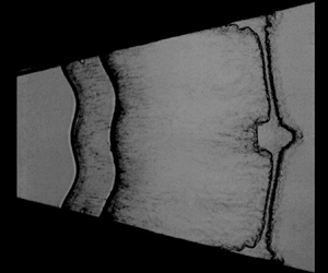
The background flow of divergent RM instability is more complicated than the planar counterpart due to the presence of geometric divergence and an unsteady, non-uniform pressure field behind the divergent shock, for which there is no theoretical solution. Thus quasi-one-dimensional (quasi-1-D) experiments corresponding to an unperturbed SF $_6$ layer surrounded by air impacted by a divergent shock are required to examine the background flow. Fortunately, these quasi-1-D experiments have been reported recently by Zhang et al. (Reference Zhang, Ding, Si and Luo2023). A sequence of schlieren images (upper) and schematic diagrams (lower) illustrating the evolution of the SF $_6$ layer driven by a cylindrical divergent shock are given in figure 2. The time origin here is defined as the moment at which the incident shock encounters the initial inner interface. At the beginning, an incident cylindrical shock (ICS) moves outwards and then collides with the inner interface (II $_1$) of the layer, bifurcating into an inward-moving reflected shock (RS $_1$) and an outward-moving transmitted shock (TS $_1$). After that, the shocked inner interface (SI $_1$) moves downstream and gradually leaves its original position. Due to shock impact, the soap film atomizes into small droplets, causing the thickening of SI $_1$ in schlieren images (122 $\mathrm {\mu }$s). The relationship between the size of the atomized soap droplets and the incident shock strength has been investigated by Cohen (Reference Cohen1991) and Ranjan et al. (Reference Ranjan, Niederhaus, Oakley, Anderson, Bonazza and Greenough2008). According to their work, the soap droplets are estimated to be approximately 30 $\mathrm {\mu }$m in radius for the present experiments, in which the incident shock Mach number is $M_i \approx 1.3$. Previous experiments with such a soap-film technique showed that the experimental results are in good agreement with numerical simulations and theoretical predictions (Wang, Si & Luo Reference Wang, Si and Luo2013; Ding et al. Reference Ding, Si, Chen, Zhai, Lu and Luo2017a; Liu et al. Reference Liu, Liang, Ding, Liu and Luo2018), which indicates a negligible influence of soap droplets on the interface evolution. Later, the outgoing TS $_1$ collides with the initial outer interface (II $_2$) of the layer, splitting into a second transmitted shock (TS $_2$) and an inward-moving rarefaction wave (RW $_1$). Note that a weak reflected shock (RS $_2$) is produced during this process, which is caused by the interaction of TS $_1$ with the protruding filaments. This reflected shock has also been observed in previous experiments, and its influence on the instability development was demonstrated to be negligible (Vandenboomgaerde et al. Reference Vandenboomgaerde, Rouzier, Souffland, Biamino, Jourdan, Houas and Mariani2018; Liang et al. Reference Liang, Liu, Zhai, Si and Wen2020a). Later, RW $_1$ accelerates the inner interface, and an outward-moving compression wave (CW $_1$) is immediately generated inside the layer (not visible in schlieren images due to the weak intensity). Afterwards, CW $_1$ compresses and accelerates the outer interface, generating a second rarefaction wave (RW $_2$), which later interacts with the inner interface again. The above wave propagation process would be repeated many times inside the layer until the reverberating waves are negligibly weak. In this work, after CW $_1$ passes across the outer interface, the waves reverberating inside the gas layer are very weak and can be ignored. The white dotted lines in figure 2 indicate the protruding filaments used to constrain the initial soap-film interfaces. A unique feature of the motion of the gas layer in a divergent geometry is that the layer becomes thinner and thinner with time due to geometric divergence, and thus exhibits an increasingly strong interface coupling effect, which will be discussed later. The inner and outer interfaces maintain a nearly cylindrical shape during the experimental time, which indicates a limited influence of boundary layer on the interface motion.

Figure 2. Schlieren images (upper) and schematic diagrams (lower) showing the developments of wave patterns and interfacial morphologies for an unperturbed SF $_6$ layer with $d_0$ = 30 mm accelerated by a cylindrical divergent shock. The white dotted lines indicate the thin filaments used to form the initial soap-film interfaces; ICS is the incident cylindrical shock; II $_i$ is the initial interface ( $i = 1,2$ refer to the inner and outer interfaces, respectively); SI $_i$ is the shocked interface; TS $_j$ is the $j$th transmitted shock; RS $_j$ is the $j$th reflected shock; RW $_1$ is the first rarefaction wave reflected from the outer interface. The unit of numbers is $\mathrm {\mu }$s.
A detailed analysis on the background flow of divergent RM instability has been reported by Zhang et al. (Reference Zhang, Ding, Si and Luo2023), and the main results are summarized below. The inner and outer interfaces of the layer move uniformly at the early stage, and their velocities can be influenced by the reverberating waves inside the layer. At late stages, the two interfaces decelerate, evidently due to the combined effects of geometric divergence and a non-uniform pressure field behind the divergent shock. The dimensionless displacements of the inner (outer) interface for gas layers of different thickness collapse well from early to late stages. A general 1-D theory applicable to an arbitrary-thickness layer is developed by taking the non-uniform pressure distribution and geometric divergence into account, which gives a good prediction of the motion of the shocked unperturbed layer in divergent geometry. For the details of the 1-D theory, readers are referred to the work of Zhang et al. (Reference Zhang, Ding, Si and Luo2023). The background flow described here would facilitate the analysis and understanding of the evolution of a perturbed gas layer.
3.2. Evolution of a perturbed gas layer
Quasi-two-dimensional (quasi-2-D) experiments, corresponding to nine types of SF $_6$ layers with various thicknesses, amplitudes and phases of the inner and outer interfaces impacted by a cylindrical divergent shock, are performed. Specifically, three thicknesses are considered: the inner interface is fixed at $R_{10} = 150$ mm, and the outer interface takes radii $R_{20} = 160, 170, 180$ mm corresponding to the layer thicknesses $d_0 = 10, 20, 30$ mm, respectively. For each thickness, various amplitudes and phases of the inner and outer interfaces are taken: case US ( $a_{10} = 0$ mm, $a_{20} = 2$ mm), case IP ( $a_{10} = a_{20} = 2$ mm) and case AP ( $a_{10} = 2$ mm, $a_{20} = -2$ mm). Here, the symbol US means that the inner interface is unperturbed while the outer interface is sinusoidally perturbed; IP means that there exist two in-phase single-mode perturbations at the inner and outer interfaces, respectively; AP means that there exist two anti-phase perturbations at the inner and outer interfaces, respectively. It should be mentioned that case SU ( $a_{10} = 2$ mm, $a_{20} = 0$ mm, i.e. the inner interface is sinusoidally perturbed while the outer interface is unperturbed) has been examined in our recent work (Zhang et al. Reference Zhang, Ding, Si and Luo2023) and is not repeated here. An unperturbed gas layer is denoted by case UU. For the convenience of expression, in this work a gas layer is named as case d10/20/30-SU/US/IP/AP, in which the first symbol denotes the layer thickness, and the second denotes the layer shape. Detailed parameters corresponding to the initial conditions for each case are listed in table 1, where the Atwood number is defined as $A=(\rho _2 - \rho _1)/(\rho _2 + \rho _1)$, with $\rho _2$ and $\rho _1$ being the gas densities inside and outside the layer, respectively. As we can see, the parameters of the perturbed layers are nearly equal to those of the unperturbed layers.
Table 1. Here,  $d_0$ is the initial thickness of the layer, $a_{10}$ ( $a_{20}$) is the initial amplitude of the inner (outer) interface, $V_{ics}$ is the velocity of the ICS, $V_{ts_j}$ is the velocity of the $j$th transmitted shock, $\Delta V_{1}$ ( $\Delta V_{2}$) is the post-shock velocity of the inner (outer) interface, mfra(SF $_6$) refers to the mass fraction of SF $_6$ inside the gas layer $A$ (
$A$ ( $A^+$) to the pre-shock (post-shock) Atwood number. The amplitude and thickness are in mm, the velocity is in m s $^{-1}$.

A key parameter in the experiment is the mass fraction of SF $_6$ inside the layer, which determines the instability growth rate at both interfaces. Although a gas concentration detector is used to measure the oxygen concentration of the gas mixture exhausted from the outflow hole, it can ensure only a high concentration of SF $_6$ inside the layer rather than measuring directly the mass fraction of SF $_6$. In this work, we estimate the mass fraction of SF $_6$ inside the layer using the following method. For a planar shock impacting a flat light/heavy interface, a 1-D flow that is composed of four uniform regions separated by a reflected shock, a transmitted shock and a contact surface, is produced. According to 1-D gas dynamics theory, we can establish the relations between the flow parameters on both sides of the reflected and transmitted shocks. With the compatibility relation at the contact surface (i.e. velocity and pressure continuity), the following equation can be derived:
 \begin{equation} \left[\frac{\left(\varLambda_2-1\right) \rho_1}{\left(\varLambda_1-1\right) \rho_2}\right]^{1 / 2} \frac{P_t-1}{\left(P_t \varLambda_2+1\right)^{1 / 2}}=\frac{P_i-1}{\left(P_i \varLambda_1+1\right)^{1 / 2}}-\left(\frac{\rho_1}{\rho_1^{\prime}}\right)^{1 / 2} \frac{P_t-P_i}{\left(P_t \varLambda_1+P_i\right)^{1 / 2}}, \end{equation}
where
 \begin{equation} \left. \begin{gathered} \varLambda_1=(\gamma_1+1)/(\gamma_1-1),\\ \varLambda_2=(\gamma_2+1)/(\gamma_2-1),\\ P_i=1+2\gamma_1/(\gamma_1+1)(M_i^2-1),\\ \rho_1/\rho_1^{\prime}=[(\gamma_1-1) M_i^2+2]/[(\gamma_1+1) M_i^2]. \end{gathered} \right\} \end{equation}
Here,  $\gamma _1$ ( $\gamma _2$) refers to the specific heat ratio inside the layer, $P_i$ ( $P_t$) to the pressure ratio across the incident shock (transmitted shock), $\rho _1^{\prime }$ to the fluid density behind the incident shock, and $M_i$ to the Mach number of the incident shock. In experiment, the gas outside the layer is pure air. The velocity of the incident shock is measured just before it collides with the inner interface, then the corresponding $M_i$ is calculated. The mass fraction of SF $_6$ is obtained by iterative method via numerical calculation. Specifically, specifying an arbitrary initial value between 0 and 1 for the mass fraction of SF $_6$ inside the layer, the flow parameters inside the layer (e.g. $\rho _2$ and $\gamma _2$) can be obtained. Substituting the known parameters into (3.1), the pressure ratio across the transmitted shock ( $P_t$) can be solved, and then the strength of the transmitted shock is available. If the calculated strength of the transmitted shock is stronger than the measured one, then the value of the mass fraction is reduced; otherwise, it is increased. This process is repeated many times until the calculated value is in good agreement with the measured one (i.e. their difference is below 0.1 %). For the unperturbed layer with $d_0 = 30$ mm, the mass fraction of SF $_6$ inside the layer is calculated to be 96 %. With this value, the flow velocity behind TS $_1$ is calculated to be 92.0 m s $^{-1}$ based on 1-D gas dynamics theory, which agrees reasonably with the experimental measurement ( $96.7\pm 1.0$ m s $^{-1}$). This demonstrates good reliability of the present calculation method. Also, it indicates a negligible influence of soap droplets on the flow.
Developments of the wave patterns and interface morphologies illustrated by sequences of schlieren images for all cases are displayed in figure 3. Here, we take case d20-US as an example to detail the evolution process. At the beginning ( $-7\,\mathrm {\mu }$s), an ICS together with an unperturbed inner interface II $_1$ and a sinusoidal outer interface II $_2$ are observed clearly, which demonstrates good feasibility of the present experimental method. The velocity of the ICS is measured to be $V_{ics} = 432.4$ m s $^{-1}$ just before it collides with the inner interface, corresponding to $M_i = 1.25$. After the ICS collides with the fast/slow inner interface, it immediately bifurcates into an upstream-moving reflected shock RS $_1$ and a downstream-moving transmitted shock TS $_1$. Note that the fast/slow interface refers to an A/B interface where the sound speed of gas A is larger than that of gas B (Samtaney, Ray & Zabusky Reference Samtaney, Ray and Zabusky1998). After that, the shocked inner interface SI $_1$ moves outwards at initial velocity $\Delta V_1 \approx 95.7$ m s $^{-1}$. As time proceeds, it maintains a cylindrical shape with no instability due to the complete alignment of ICS with the initial interface. Afterwards, the cylindrical TS $_1$ collides with the sinusoidal outer interface, immediately bifurcating into a second transmitted shock TS $_2$ and an upstream-moving rarefaction wave RW $_1$ (143 $\mathrm {\mu }$s). Note that RW $_1$ possesses an identical perturbation phase relative to the outer interface, while TS $_2$ presents an opposite phase. After the impact of TS $_1$, the amplitude of the outer interface reduces gradually to zero (i.e. phase reversal) and then increases gradually with an opposite phase. Later, the disturbed RW $_1$ stretches and accelerates the inner interface, seeding a visible perturbation on the inner interface (260 $\mathrm {\mu }$s). It indicates that for a heavy gas layer, the initial perturbation of the outer interface can be transferred to the unperturbed inner interface through RW $_1$. This differs from the SU case, where the unperturbed outer interface suffers a negligible influence of reverberating waves and thus maintains a nearly cylindrical shape during a long period of time (Zhang et al. Reference Zhang, Ding, Si and Luo2023). During the interaction of RW $_1$ with the inner interface, an outward-moving compression wave CW $_1$ is generated (not visible schlieren images due to the weak intensity), which later compresses and accelerates the shocked outer interface SI $_2$. At late times, the inner and outer interfaces increase in amplitude with an identical phase ( $477\unicode{x2013} 878$ $\mathrm {\mu }$s). The time origin for the evolution of a perturbed layer is defined as the moment at which the incident shock arrives at the mean position of the inner interface.

Figure 3. Schlieren images showing the developments of wave patterns and interfacial morphologies for all cases. The white dotted lines indicate the thin filaments used to form the initial soap-film interfaces. The symbols are the same as those in figure 2. The unit of numbers is  $\mathrm {\mu }$s.
For case d20-IP, the rarefaction wave RW $_1$ is in phase with the inner interface, thus their interaction lasts a relatively shorter period of time. As a result, RW $_1$ stretches (or amplifies) the inner interface amplitude to a lesser extent than in case d20-US, which is confirmed by the quantitative data hereinafter. After the impact of TS $_1$, the outer interface first reverses phase, and then presents an anti-phase perturbation relative to the inner interface. For this case, interface coupling inhibits the instability growth at each interface according to Mikaelian (Reference Mikaelian1985, Reference Mikaelian1995). For case d20-AP, RW $_1$ is out of phase with the inner interface and thus takes a longer period of time to passes across the inner interface. As a result, it stretches (or amplifies) the inner interface amplitude to a larger extent than the IP and US cases (253 $\mathrm {\mu }$s). Also, after phase reversal, the outer interface presents an in-phase perturbation relative to the inner interface. For this case, interface coupling promotes the instability growth at each interface of the layer. This explains reasonably the observation that the instability growth in the AP case is quicker than in the IP and US cases (770 $\mathrm {\mu }$s). It manifests that the phase difference between the two interfaces significantly affects the instability growth at a gas layer. The interface contours at typical moments for the IP, AP and US cases with thickness 20 mm are extracted from the experimental schlieren images with a post-processing program written in MATLAB language, as shown in figure 4. This makes it much easier to assess the phase difference between the two interfaces on the layer evolution. Results of various layer thicknesses show that the layer thickness produces an evident influence on the growth rate of the instability at each interface, but cannot alter the eventual perturbation phases of the two interfaces. For all nine cases, the gas layer becomes thinner and thinner with time due to geometric divergence. In particular, the inner and outer interfaces coalesce to one for the $d_0=$ 10 mm layers. To show the evolution process clearly, sketches of the wave patterns and interfacial morphologies at typical moments for the US, IP and AP layers with the same thickness ( $d_0 = 20$ mm) are given in figure 5.

Figure 4. The interface contours extracted from schlieren images at typical moments for the IP, AP and US cases with thickness 20 mm. The unit of numbers is  $\mathrm {\mu }$s.

Figure 5. Sketches of the wave patterns and interface morphologies at typical moments for different cases. Here,  $\Delta V_2$ ( $\Delta V_2^*$) is the velocity of the outer interface immediately after the impact of TS $_1$ (CW $_1$). The other symbols are the same as those in figure 2.
3.3. Instability growth at the early stage
In this work, we divide qualitatively the instability growth into early and late stages. Here, the early stage refers to the phase at which the instability growth suffers a considerable influence of waves (i.e. a compressibility effect is evident), while the late stage refers to the stage at which the wave effects are weak, and interface coupling dominates the instability growth.
3.3.1. Growth of the inner interface amplitude
Variations of the amplitude of the inner interface versus time for all cases are plotted in figures 6(a,c,e). For each case, the amplitude of the inner interface first experiences a sudden drop due to shock compression and then grows almost linearly with time before the arrival of RW $_1$. The quasi-linear growth here indicates that geometric divergence produces a negligible influence on the instability growth at the early stage, which is consistent with the previous finding (Li et al. Reference Li, Ding, Zhai, Si, Liu, Huang and Luo2020b; Zhang et al. Reference Zhang, Ding, Si and Luo2023). The experimental data of the SU layers with various thicknesses from Zhang et al. (Reference Zhang, Ding, Si and Luo2023) are also given in figures 6(a,c,e) for comparison. Comparison among the SU, IP and AP cases (the initial inner interface remains the same for the three cases) for the amplitude growth of the inner interface can reveal the influence of phase difference between the two interfaces on the inner interface development. As we can see, for each thickness, the instability growths at the inner interface for the SU, IP and AP cases collapse quite well before the arrival of RW $_1$, which indicates a negligible interface coupling effect. This can be interpreted from the perspective of pressure disturbances. For compressible fluids, the perturbation at one interface feeds through to another interface via pressure disturbance, which propagates at the sound speed and thus cannot cross the reverberating waves (such as RW $_1$ and CW $_1$) to influence the other interface. Thus, before the arrival of RW $_1$, the evolution of the inner interface suffers no influence of the outer interface, and vice versa (i.e. there is no interface coupling effect at this time). This also explains the observation that the classical Bell (Reference Bell1951) theory developed for cylindrical RM instability at a single interface gives a good prediction (dashed line) of the instability growth at the inner interface before the arrival of RW $_1$ for all cases. When RW $_1$ arrives, the inner interface presents a much quicker instability growth than the prediction of Bell theory, which indicates that RW $_1$ promotes the instability growth at the inner interface. It is found that for gas layers with an identical thickness, RW $_1$ promotes the instability growth to a large extent for the AP case, to a moderate extent for the SU case, and to a small extent for the IP case. In particular, for case d10-IP, the RW $_1$ event inhibits the instability growth. This implies that the effect of RW $_1$ on the growth of the inner interface depends heavily on the initial perturbation phases of the two interfaces.

Figure 6. Comparison of the amplitudes of (a,c,e) the inner interface and (b,d,f) the outer interface among different cases. The dashed line refers to the prediction of the Bell–RT model. The bold solid line refers to the prediction of the Bell–RT-m model that considers the interface stretching and RT instability caused by RW $_1$ in (a,c,e), and to the instability growth caused by CW $_1$ in (b,d,f). The symbols are the same as those in figure 2.
Here, we give a quantitative estimation of the influence of RW $_1$ on the instability growth, which is crucial for understanding and modelling the instability growth of a fluid layer at the early stage. Since the layer thickness is much smaller than its radius (i.e. $d \ll R$), RW $_1$ experiences only a subtle change in velocity while propagating inside the layer. Thus the motion of RW $_1$ can be assumed as that in a planar geometry, as sketched in figure 7(a). The time at which TS $_1$ encounters the outer interface is defined as $t_{ts_1}$, the time at which RW $_1$ is generated as $t^0_r$, and the time at which RW $_1$ interacts with the shocked inner interface as $t_{rw_1}$. Then $t_{ts_1}$, $t^0_r$ and $t_{rw_1}$ can be estimated by
 \begin{equation} \left. \begin{gathered} t_{ts_1}=t_r^0=\displaystyle \frac{d_0}{V_{ts_1}} ,\\ t_{rw_1}=\displaystyle \frac{d_0(V_{ts_1}-\Delta V_1+c_1)}{c_1 \, V_{ts_1}}=t_{ts_1}+\displaystyle \frac{d_0}{c_1}\left(1-\displaystyle \frac{\Delta V_1}{V_{ts_1}}\right) , \end{gathered} \right\} \end{equation}
where  $c_1$ is the sound speed of the gas behind TS $_1$ inside the layer. According to 1-D gas dynamics theory, the width of RW $_1$ (defined as the distance between its head and tail) at the moment when it encounters the inner interface is $L = (\gamma +1)(\Delta V_2 - \Delta V_1)d^*/(2c_1)$, where $\gamma$ is the specific heat ratio inside the layer, and $d^*=d_0(1-\Delta V_1/V_{ts_1})$ is the layer thickness at $t_{ts_1}$. According to Morgan, Likhachev & Jacobs (Reference Morgan, Likhachev and Jacobs2016), it can be assumed that RW $_1$ accelerates the inner interface with a constant acceleration ( $g_{rw_1}$). Then $\Delta t_g$ (i.e. the acceleration duration) and $g_{rw_1}$ can be calculated by $\Delta t_g=2L/(2c_1+\Delta V_1^*-\Delta V_1)$ and $g_{rw_1}=(\Delta V_1^*-\Delta V_1)/ \Delta t_g$, respectively, where $\Delta V_1^*$ is the velocity of the inner interface after the impact of RW $_1$. The relevant parameters for the unperturbed layers of different thicknesses are listed in table 2. Note that for a perturbed layer, the interface acceleration caused by RW $_1$ would induce RT instability, which can evidently promote the instability growth (Liang et al. Reference Liang, Zhai, Luo and Wen2020b; Liang & Luo Reference Liang and Luo2021a).

Figure 7. Schematic diagrams showing (a) the wave propagations and interface motions for a shock wave impacting a heavy gas layer, and (b) the detailed process of the distorted RW $_1$ passing through the inner interface. Here, $d^*$ is the layer thickness just before TS $_1$ collides with II $_2$,
$_2$,  $\Delta V_1$ ( $\Delta V_2$) is the post-shock velocity of the inner (outer) interface, $\Delta V_1^*$ ( $\Delta V_2^*$) is the velocity of the inner (outer) interface after the impact of RW $_1$ (CW $_1$), $L$ is the distance between the head and tail of RW $_1$ just before it impacts the inner interface, and $c_1$ ( $c_2$) denotes the sound speed of the fluid behind TS $_1$ (RW $_1$) inside the layer. The symbols are the same as those in figure 2.
Table 2. The key parameters for the interactions of a divergent shock with unperturbed layers of different thicknesses. Here,  $t_{ts_1}$ and $t_{cw_1}$ are the times when TS $_1$ and CW $_1$ encounter the outer interface, respectively, $t_{rw_1}$ is the time when RW $_1$ encounters the inner interface, $\Delta V^*_1$ ( $\Delta V^*_2$) is the velocity of the inner (outer) interface after the impact of RW $_1$ (CW $_1$), $c_1$ ( $c_2$) is the sound speed of the fluid behind TS $_1$ (RW $_1$) inside the layer, $\gamma$ is the specific heat ratio inside the layer, $L$ is the width between the head and tail of RW $_1$ when it encounters the inner interface, $\Delta t_g$ is the time duration between the inner interface passing through the head and tail of RW $_1$, and $g_{rw_1}$ is the average acceleration of the inner interface caused by RW $_1$. The units are $\mathrm {\mu }$s, mm, m s $^{-1}$ and m s $^{-2}$ for the time, length, speed and acceleration, respectively.

Besides interface acceleration, RW $_1$ also stretches the interface, causing a quick increment in interface amplitude (called the interface stretching effect in this work). The parameters listed in tables 1 and 2 enable us to quantify the interface stretching effect. As shown in figure 5, for any of the US, IP or AP cases, after TS $_1$ collides with the sinusoidal outer interface, a disturbed RW $_1$ that presents an in-phase perturbation relative to the outer interface is generated immediately. The initial amplitudes of the leading front ( $a_{rh}^0$) and trailing front ( $a_{rt}^0$) of RW $_1$ can be calculated by
 \begin{equation} \left. \begin{gathered}
a_{rh}^0=a_{20}+\displaystyle\frac{c_1-\Delta
V_1}{V_{ts_1}}(a_{20}-a_{ts_1}(t_{ts_1})),\\
a_{rt}^0=a_{20}+\displaystyle\frac{c_2-\Delta
V_2}{V_{ts_1}}(a_{20}-a_{ts_1}(t_{ts_1})),
\end{gathered} \right\}
\end{equation}
\begin{equation} \left. \begin{gathered}
a_{rh}^0=a_{20}+\displaystyle\frac{c_1-\Delta
V_1}{V_{ts_1}}(a_{20}-a_{ts_1}(t_{ts_1})),\\
a_{rt}^0=a_{20}+\displaystyle\frac{c_2-\Delta
V_2}{V_{ts_1}}(a_{20}-a_{ts_1}(t_{ts_1})),
\end{gathered} \right\}
\end{equation}
where  $a_{ts_1}(t_{ts_1})$ is the amplitude of TS $_1$ at $t_{ts_1}$. Since there is no theoretical solution for the variation of a rippled shock amplitude in divergent geometry, $a_{ts_1}(t_{ts_1})$ is measured from experiment in this work. The calculated values of $a_{r h}^0$ and $a_{r t}^0$ are nearly equal, thus $a_{r h}^0$ can represent approximately the amplitude of RW $_1$ in this work, as listed in table 3. Also, considering that the amplitude of RW $_1$ undergoes only a subtle variation inside the layer, it can be assumed that $a_{rh}(t_{rw_1})=a_{rt}^0$. As sketched in figure 7(b), during the interaction of RW $_1$ with the inner interface, RW $_1$ accelerates first the bubble of the inner interface and then the spike, producing a velocity difference between the tips of the bubble and the spike. This leads to a quick increment in interface amplitude, i.e. the interface stretching effect. The time duration between the moments at which the crest and trough of the leading front of RW $_1$ encounter respectively the inner interface is defined as $\Delta t_s$, which can be calculated by
 \begin{equation} \Delta t_s=\displaystyle\frac{2\left(a_1(t_{rw_1})-a_{rh}\right)}{c_1}. \end{equation}
Thus the time duration of RW $_1$ passing across the inner interface is $\Delta t_{rw_1} = \vert \Delta t_s \vert + \Delta t_g$, as sketched in figure 7(b). The amplitude increment caused by the stretching effect ( $\Delta a_s^{rw}$) and the corresponding average growth rate ( $\dot a_s^{rw}$) can be estimated respectively by
 \begin{equation} \left. \begin{gathered} \Delta a_s^{rw} =\displaystyle\frac{\Delta t_s\left(\Delta V_1^*-\Delta V_1\right)}{2} ,\\ \dot{a}_s^{rw} =\displaystyle\frac{\Delta a_s^{r w}}{\left|\Delta t_s\right|+\Delta t_g}. \end{gathered} \right\} \end{equation}
The calculation results for all cases are listed in table 3. It is seen that for the IP (AP) case, the influences of RW $_1$ on the instability growth at the inner interface are the weakest (strongest) due to the shortest (longest) action time.
Table 3. The relevant parameters for all perturbed layers. Here,  $a_{ts_1}(t_{ts_1})$ refers to the amplitude of TS $_1$ at the time $t_{ts_1}$, $a_{rh}^0$ ( $a_{cw_1}^0$) is the initial amplitude of RW $_1$ (CW $_1$), $a_1(t_{rw_1})$ ( $a_2(t_{cw_1})$) is the amplitude of the inner (outer) interface at the time $t_{rw_1}$ ( $t_{cw_1}$), $\Delta t_s$ is the time duration between the moments when the peak and trough of RW $_1$ respectively encounter the inner interface, $\Delta t_{rw_1}$ ( $\Delta t_{cw_1}$) is the time duration for RW $_1$ (CW $_1$) passing through the inner (outer) interface, $\dot a_s^{rw}$ represents the average growth rate caused by interface stretching, and $\dot a_1$ ( $\dot a_2$) is the growth rate of the inner (outer) interface after the impact of RW $_1$ (CW $_1$). The units are $\mathrm {\mu }$s, mm and m s $^{-1}$ for the time, length and speed, respectively.

To reveal the influence of layer thickness, here we define a critical thickness  $d_{cr}$ for the gas layer in which the interface amplitude is equal to the amplitude of RW $_1$ when they meet, i.e. $a_1(t_{rw_1})=a_{rh}(t_{rw_1})$. There are three possible situations, depending on the layer thickness: $d_0 < d_{cr}$, $d_0 = d_{cr}$ or $d_0 > d_{cr}$. As sketched in figure 8, for $d_0< d_{cr}$ ( $\Delta t_s < 0$), the trough of the inner interface (point $A$) is first accelerated by RW $_1$, thus both the interface stretching effect and RT instability induce a negative growth rate, i.e. the instability growth is inhibited. For $d_0=d_{cr}$ ( $\Delta t_s = 0$), the trough and crest of the inner interface (points $A$ and $B$) are accelerated simultaneously by RW $_1$, i.e. the stretching effect disappears. Also, for this situation, RT instability is the weakest due to the shortest duration of RW $_1$ passing through the interface. For $d_0>d_{cr}$ ( $\Delta t_s > 0$), point $B$ is first accelerated by RW $_1$, and both the interface stretching effect and RT instability induce a positive growth rate, i.e. the instability growth is promoted.

Figure 8. Three situations for (i) the interaction of distorted RW $_1$ with the inner interface in case IP, and (ii) the equivalent diagrams considering RW $_1$ is undisturbed. Here, $d_0$ refers to the initial layer thickness, $d_{cr}$ is the critical thickness of the layer (where the amplitudes of RW $_1$ and inner interface are equal at the time $t_{rw_1}$), $g_{rw_1}$ is the average acceleration of the inner interface caused by RW $_1$, and $A$ and $B$ are the points on the tip of the spike and the bubble, respectively. The other symbols are the same as those in figure 2.
Here, we give a quantitative estimation of the critical thickness  $d_{cr}$. Since geometric divergence has a negligible influence on the layer evolution at the early stage (Luo et al. Reference Luo, Zhang, Ding, Si, Yang, Zhai and Wen2018), the amplitude of the inner interface just before the impact of RW $_1$ can be approximated as
 \begin{equation} a_1(t_{rw_1})=a_1^++\dot{a}_0\, t_{rw_1}, \end{equation}
where  $a_1^+=a_{10} (1-\Delta V_1/V_{ics} )$ is the post-shock amplitude, and $\dot a_0 \approx 8.0$ m s $^{-1}$ (obtained by a linear fit of experimental data) is the post-shock growth rate at the inner interface. Letting $a_1(t_{rw_1})= a_{rh} (t_{rw_1})$, with (3.10), (3.4) and (3.7), $d_{cr}$ is derived as
 \begin{align} d_{cr}=\displaystyle\frac{c_1}{\dot{a}_0}\left[\left(a_{20}-a_{10}\right)+\displaystyle\frac{a_{10} V_{ts_1} c_1}{V_{ics}\left(V_{ts_1}+c_1-\Delta V_1\right)}-\displaystyle\frac{c_1-\Delta V_1}{V_{ts_1}+c_1-\Delta V_1} \int_0^{t_{ts_1}} \alpha(t) \,{\rm d}t\right], \end{align}
where  $\alpha (t)$ refers to the growth rate of the amplitude of TS $_1$. Since the variation of $\alpha (t)$ in divergent geometry is very complex, for which there is no theoretical solution, it is hard to give a theoretical value for $d_{cr}$. Here, we consider two limiting cases: for a very thin layer in which the variation of $\alpha (t)$ is negligibly small, there is $\alpha (t) \approx 0$; for a very thick layer in which TS $_1$ has almost recovered to a cylindrical shock at $t_{ts_1}$, there is $\int _0^{t_{ts_1}}\alpha (t)\,\textrm{d}t \approx -a_{10}(1-V_{ts_1}/V_{ics})$. Substituting the relevant parameters into (3.8) (such as case d20-UU in tables 1 and 2), $d_{cr}$ is estimated to be 11.0 mm and 15.8 mm for these two limiting situations, respectively. Hence, for a finite-thickness layer, the critical thickness is within the range $11.0 < d_{cr} < 15.8$ mm. Under the current experimental conditions, if $d_0 < 11.0$ mm, then the instability growth at the inner interface would be inhibited by RW $_1$, while if $d_0 > 15.8$ mm, then the instability growth would be promoted. The present analysis explains reasonably the suppression of RW $_1$ on the instability growth at the inner interface for case d10-IP, in which $d_0 < d_{cr}$.
Taking both RT instability and the interface stretching effect caused by the rarefaction wave into account, recently Zhang et al. (Reference Zhang, Ding, Si and Luo2023) proposed a modified Bell–RT model (called the Bell–RT-m model), which is expressed as
 \begin{align} a(t)=a_0^++\dot{a}_0 R_0^2 \int_{t_0^+}^t \frac{1}{R^2(t^{\prime})} \,{\rm d}t^{\prime}+(n A-1) \int_{t_0^+}^t\left(\frac{1}{R^2(t^{\prime})} \int_{t_0^+}^{t^{\prime}} a R \ddot{R} \,{\rm d}t^{\prime \prime}\right) {\rm d}t^{\prime}+\dot{a}_s^{rw}(t-t_{rw_1}). \end{align}
This model has been validated by experiment for the case of a uniform rarefaction wave accelerating a perturbed interface (Zhang et al. Reference Zhang, Ding, Si and Luo2023). The present experimental results provide an opportunity to examine the validity of the model for more complex situations, e.g. a distorted rarefaction wave interacts with a perturbed interface. As can be seen in figures 6(a,c,e), (3.9) that takes an average acceleration ( $\ddot {R} = g_{rw_1}$) and an average stretching growth rate ( $\dot {a}_s^{rw}$) well reproduces the instability growth caused by RW $_1$ for most cases. An exception is the d30-AP case, in which the perturbation growth is overestimated. The reason is discussed below. As we know, the RT effect plays a role only when RW $_1$ accelerates the interface. For case d30-AP, the inner interface presents a relatively large amplitude just before the impact of RW $_1$, and also its perturbation phase is opposite to that of RW $_1$. As a result, the passage of RW $_1$ across the inner interface in case d30-AP lasts a longer period of time than in the other cases. As sketched in figure 7(b), for this case the crest of RW $_1$ has been far away from the inner interface when the trough of RW $_1$ encounters the inner interface. In the calculation of (3.9), it is thought that RT instability acts on the interface at the whole stage of the interaction of RW $_1$ with the interface, which is not the case for the real situation. This may be the reason for the overestimation of the instability growth for case d30-AP. It is seen that the inhibition of the instability growth at the inner interface caused by RW $_1$ in case d10-IP is also reproduced by the Bell–RT-m model. The present analysis suggests that the Bell–RT-m model is valid for cases with various perturbation phases and thicknesses except the AP case with a relatively large thickness.
3.3.2. Growth of the outer interface amplitude
Temporal variations of the amplitude of the outer interface for the US, IP and AP cases (the initial outer interface remains the same for the three cases) are given in figures 6(b,d,f). As we can see, the amplitude of the outer interface suffers a sudden drop due to the compression of TS $_1$. The interaction of the distorted TS $_1$ with the sinusoidal outer interface here belongs to complex non-standard RM instability (i.e. a rippled shock impacts a perturbed interface), which involves more regimes than the simple non-standard RM instability (i.e. a rippled shock impacts an unperturbed interface) and the conventional standard RM instability (a uniform shock impacts a perturbed interface) (Ishizaki et al. Reference Ishizaki, Nishihara, Sakagami and Ueshima1996; Zou et al. Reference Zou, Liu, Liao, Zheng, Zhai and Luo2017, Reference Zou, Al-Marouf, Cheng, Samtaney, Ding and Luo2019; Li et al. Reference Li, Ding, Luo and Zou2022a). Here, we analyse the perturbation growth caused by TS $_1$ in the view of baroclinic vorticity, which is a major driving force for the instability growth. Sketches in the first row of figure 5 show the interaction of TS $_1$ with the outer interface for the US, IP and AP cases. For the IP case, TS $_1$ is in phase with the outer interface (i.e. there is a small angle between the density gradient across the interface and the pressure gradient at TS $_1$), thus weaker baroclinic vorticity is deposited at the interface than in the US case. Also, the interface is compressed to a lower extent as compared to the US case. This leads to a slower instability growth at the early stage in the IP case than in the US case. For the AP case, TS $_1$ is out of phase with the outer interface, thus stronger baroclinic vorticity is deposited at the outer interface than in the US case. Also, the interface is compressed to a larger extent. These lead to a quicker instability growth at the early stage than in the US case. It should be stressed that for the large-thickness layers such as case d30-IP and case d30-AP, TS $_1$ has recovered to a cylindrical divergent shock just before it arrives at the outer interface, thus the instability growths at the outer interface collapse well before the impact of CW $_1$, as shown in figure 6(f). After the impact of CW $_1$, the AP case presents a quicker instability growth than in the US case, whereas the IP case presents a slower instability growth. The present results indicate that CW $_1$ also affect the instability growth.
Similar to RW $_1$, CW $_1$ also experiences a subtle change in velocity while propagating inside the layer, thus its motion can be assumed as that in a planar geometry, as sketched in figure 7(a). The time at which CW $_1$ is generated is defined as $t^0_c$, and the time at which CW $_1$ interacts with the shocked outer interface is defined as $t_{cw_1}$. Then $t^0_c$ and $t_{cw_1}$ can be estimated by
 \begin{equation} \left. \begin{gathered} t_c^0=t_{rw_1}=t_{ts_1}+\displaystyle \frac{d_0}{c_1}\left(1-\displaystyle \frac{\Delta V_1}{V_{ts_1}}\right), \\ t_{cw_1}=t_{rw_1}+\displaystyle \frac{d_0}{c_2}\left(1-\displaystyle \frac{\Delta V_1}{V_{ts_ 1}}\right)\left(1+\displaystyle \frac{\Delta V_2-\Delta V_1}{c_1}\right), \end{gathered} \right\} \end{equation}
where  $c_2$ is the sound speed of the gas behind RW $_1$ inside the layer. Note that CW $_1$ possesses an initial perturbation, and its amplitude can be approximated as
 \begin{equation} a_{cw_1}^0=a_1(t_{rw_1})+\displaystyle\frac{a_1(t_{rw_1})-a_{rh}(t_{rw_1})}{c_1}\left(c_2+\Delta V_2-\Delta V_1\right). \end{equation}
The amplitude of CW $_1$ can be assumed as constant during the short period of propagation inside the layer, i.e. $a_{cw_1}(t_{cw_1}) \approx a_{cw_1}^0$. As shown in figure 5, after the impact of CW $_1$, the velocity of the outer interface increases from $\Delta V_2$ to $\Delta V_2^*$. Meanwhile, the outer interface increases continuously in amplitude due to the velocity difference between the tips of the spike and the bubble until CW $_1$ passes completely across the interface. It should be mentioned that the outer interface is reversing phase during its interaction with CW $_1$. As we can see, the instability growth at the outer interface is promoted for the US and AP cases in which the CW $_1$ is out of phase with the initial outer interface, whereas it is inhibited for the IP case in which the CW $_1$ is in phase with the initial outer interface. The time duration for CW $_1$ passing through the outer interface can be estimated by $\Delta t_{cw_1}=2[a_{cw_1}(t_{cw_1} )-a_2(t_{cw_1})]/c_2$. As listed in table 3, the effect of CW $_1$ on the outer interface for the AP case is much greater than that of the US and IP cases due to its longer action time. Then the influence of CW $_1$ on the growth of the outer interface can be estimated as $\Delta a_2^{cw}=(\Delta V_2^* - \Delta V_2)\,\Delta t_{cw_1}/2$. The results indicate that the amplitude variation in the US and IP cases is much smaller than that of the AP case. In particular, it is almost equal in size to the spatial resolution of schlieren images and thus can be ignored. We assume that the interface amplitude increases linearly with time during the short stage of the interaction of CW $_1$ with the outer interface. Thus the growth rate of the outer interface can be obtained by a linear superposition of the growth rate just before the arrival of CW $_1$ ( $\dot a_2$, obtained by experimental fitting and listed in table 3) and the average growth rate caused by CW $_1$ ( $\dot a^{cw}=(\Delta V_2^*-\Delta V_2)/2$). This gives a good prediction of the amplitude growth of the outer interface at the CW $_1$-affection stage for the AP case, as shown by the thick solid lines in figures 6(b,d,f). It can be concluded here that the influence of RW $_1$, TS $_1$ and CW $_1$ on the instability growth can be modulated by changing their perturbation phase relative to the interface (i.e. by changing the initial phase difference between the inner and outer interfaces). In particular, as has been found by Zhang et al. (Reference Zhang, Ding, Si and Luo2023), the effect of reverberating waves on divergent RM instability is more evident than that in planar and convergent RM instabilities, thus the instability modulation through waves would be more efficient for divergent RM instability.
3.4. Instability growth at the late stage
As the waves are away from the interface, the flow near the gas layer is nearly incompressible (i.e. the effect of waves is negligible) and interface coupling becomes evident, which dominates the late-stage instability growth. In particular, for RM instability in a divergent geometry, the gas layer becomes thinner and thinner with time, producing an increasingly strong interface coupling effect. As shown in figure 9, for each thickness, the AP case presents the largest growth rate at late stages, the SU case presents the medium growth rate, and the IP case presents the smallest growth rate. This is ascribed mainly to the various interface coupling effects in these cases. Specifically, for the IP case, the inner and outer interfaces present opposite phases at late stages, thus their evolutions are inhibited by each other due to interface coupling (Mikaelian Reference Mikaelian1995). For the AP case, the inner and outer interfaces present an identical phase at late stages, and their evolutions are promoted by interface coupling. Thus for the IP case, the perturbation on the inner/outer interface presents a slower instability growth than the SU/US case, but the AP case presents a quicker instability growth than the SU/US case. This finding is consistent qualitatively with that in planar (Liang & Luo Reference Liang and Luo2021a, Reference Liang and Luo2022) and convergent (Li et al. Reference Li, Ding, Luo and Zou2022a) RM instabilities. Recently, Matsuoka & Nishihara (Reference Matsuoka and Nishihara2023) also found the dependence of phase difference on the instability growth from the perspective of vortex sheet dynamics. It should be stressed that the instability growth trends for various layer thicknesses are generally similar, which indicates that the layer thickness is a relatively minor factor compared to the phase difference between the two interfaces within the parameter space considered in this work.

Figure 9. Comparison of the amplitudes of (a,c,e) the inner interface and (b,d,f) the outer interface between experiments and predictions for all cases. The dashed line refers to the prediction of the Bell–RT model that takes the post-wave (RW $_1$ and CW $_1$) growth rate as the initial value; the bold solid line refers to the prediction of the Bell–RT-m model; the thin solid line refers to the prediction of the Bell–RT-C model. The vertical dotted line denotes the times of reverberating waves interacting with the inner and outer interfaces. The symbols are the same as those in figure 2.
Under the incompressible, inviscid, irrotational fluid assumption, Mikaelian (Reference Mikaelian2005) has derived a set of linear equations for RM instability at an arbitrary number ( $N$) of cylindrical layers:
 \begin{align} (\rho_{i+1}-\rho_i)\,\displaystyle\frac{{\rm d}}{{\rm d} t}(R_i \dot{R}_i a_i)=R_i^{n+1}\left(\rho_{i+1}\,\displaystyle\frac{{\rm d} B_{i+1}}{{\rm d} t}-\rho_i\, \displaystyle\frac{{\rm d} B_i}{{\rm d} t}\right) +(R_i)^{1-n}\left(\rho_{i+1}\, \displaystyle\frac{{\rm d} C_{i+1}}{{\rm d}t} - \rho_i\,\frac{{\rm d} C_i}{ {\rm d} t}\right), \end{align}
where
 \begin{equation} \left. \begin{gathered} B_i=\displaystyle\frac{1}{n\left[R_i^{2 n}-\left(R_{i-1}\right)^{2 n}\right]}\left[R_{i-1}^n\, \displaystyle\frac{{\rm d}}{{\rm d} t}(R_{i-1} a_{i-1})-R_i^n\,\displaystyle\frac{{\rm d}}{{\rm d} t}(R_i a_i)\right],\\ C_i=B_i(n \rightarrow -n). \end{gathered} \right\} \end{equation}
Here,  $i=1,\ldots,N$ refers to the serial number of the cylindrical layer from inside to outside (the thickness of the $N$th cylindrical layer tends to infinity), $\rho _i$ is the fluid density in the $i$th layer, $\dot R$ ( $\ddot R$) is the first (second) derivative of the interface radius ( $R$) with time, and $C_1=B_N = 0$. For $N=2$, there is only one interface and the equation reduces to
 \begin{equation} \displaystyle\frac{{\rm d}^2 a}{{\rm d} t^2}+\frac{2 \dot{R}}{R}\,\displaystyle\frac{{\rm d} a}{{\rm d} t}-(n A-1)\,\displaystyle\frac{\ddot{R}}{R}\,a=0, \end{equation}
which is called the Bell (Reference Bell1951) equation. Treating the shock impact as an impulse function (i.e.  $\ddot R = \delta (t)\,\Delta V$) and then integrating the Bell equation, the interface amplitude at any time $t$ is obtained as
 \begin{align} a(t)=a_{0}^++\dot{a}_{0} R_{0}^{2} \int_{t_{0}^+}^{t} \frac{1}{R^{2}(t^{\prime})} \,{\rm d}t^{\prime}+(n A-1) \int_{t_{0}^+}^{t}\left(\frac{1}{R^{2}(t^{\prime})} \int_{t_{0}^+}^{t^{\prime}} a(t^{\prime \prime})\,R(t^{\prime \prime})\,\ddot{R}(t^{\prime \prime}) \,{\rm d} t^{\prime \prime}\right) {\rm d}t^{\prime}, \end{align}
where  $a^+_0$ refers to the post-shock amplitude, $t^+_0$ to the time just after the shock passage, and $\dot a_0$ to the initial growth rate at $t^+_0$. For brevity, (3.15) is termed the Bell–RT model. It has been demonstrated that the Bell–RT model is able to give a reasonable prediction of the instability growth at a single sinusoidal interface in divergent/convergent geometry (Ding et al. Reference Ding, Li, Sun, Zhai and Luo2019; Li et al. Reference Li, Ding, Zhai, Si, Liu, Huang and Luo2020b). For the gas layer considered in this work, there are three cylindrical layers, i.e. $N = 3$. Performing a lengthy algebraic operation of (3.12), the differential equations for the instability growths at the inner and outer interfaces are available, expressed as
 \begin{equation} \left. \begin{gathered} E_1 \ddot{a}_1+F_1 \dot{a}_1+H_1 a_1+K_1 \ddot{a}_2+L_1 \dot{a}_2+P_1 a_2=0, \\ E_2 \ddot{a}_1+F_2 \dot{a}_1+H_2 a_1+K_2 \ddot{a}_2+L_2 \dot{a}_2+P_2 a_2=0. \end{gathered} \right\} \end{equation}
Here,  $E_{1/2}, F_{1/2}, H_{1/2}, K_{1/2}, L_{1/2}, P_{1/2}$ are the algebraic expressions of the relevant interface parameters ( $R, \dot R, \ddot R, n, \rho _i$), as given in Appendix A. Also, $a_1$ and $a_2$ are the amplitudes of the inner and outer interfaces, respectively, and $\dot a$ ( $\ddot a$) is the first (second) derivative of the amplitude with respect to time. Equations (3.16), which involve the interface coupling effect, are termed the Bell–RT-C model in this work. Since it is difficult to derive a theoretical solution for (3.16), here a program is developed to solve numerically the Bell–RT-C model. To verify the reliability of the program, the Bell–RT-C model with a very large azimuthal mode number $n$ for which the two interfaces nearly decouple (Mikaelian Reference Mikaelian1995, Reference Mikaelian2005) is solved first. As expected, the Bell–RT-C model gives almost the same prediction as that of (3.15) for each interface in this case, which demonstrates the accuracy of the program.
To the authors’ knowledge, the theory of Mikaelian (Reference Mikaelian2005) has never been validated by experiment. A major reason is that it is very difficult to obtain high-fidelity experimental results for RM instability at two or more well-controlled interfaces in a cylindrical geometry. Another reason is that the theory of Mikaelian (Reference Mikaelian2005) is suitable only for the instability growth within the linear regime, which brings more challenge to experiments in which nonlinearity is usually present. We state that the divergent RM instability presents much weaker nonlinearity than the planar and convergent counterparts (Li et al. Reference Li, Ding, Zhai, Si, Liu, Huang and Luo2020b), and thus provides a natural opportunity to examine the validity of the Mikaelian theory. Also, the gas layer in a divergent geometry becomes thinner and thinner with time, producing an increasingly strong interface coupling effect. Hence divergent RM instability at a gas layer considered in this work is an excellent configuration for examining the Bell–RT-C model.
Comparisons between the experiment and the prediction of the Bell–RT-C model for the variations of the amplitudes of the inner and outer interfaces versus time at late stages are given in figure 9, where the prediction of the Bell–RT model (the dashed line) is also given. Note that the parameters of the interfaces for the undisturbed layers ( $\dot R$ and $\ddot R$) are adopted for the mode prediction. The growth rate of the inner/outer interface after the impact of RW $_1$/CW $_1$ ( $\dot a_1$, $\dot a_2$ in table 3) obtained by a linear fit of experimental data is taken as the initial value. After the impact of RW $_1$, the inner interface presents diverse instability growths depending on the phase difference between the inner and outer interfaces. Specifically, for each layer thickness, the instability growth at the inner/outer interface for the AP case is much quicker than that of the SU/US case, whereas the instability growth at the inner/outer interface for the IP case is much slower than in the SU/US case. As the gas layer becomes thinner, the instability growth at the inner interface for the AP case is promoted to a larger extent due to the stronger interface coupling. Nevertheless, for the IP case, the thinner the gas layer, the slower the instability growth at the inner and outer interfaces. It is found that the Bell–RT-C model (thin solid line) well reproduces the instability growths at both the inner and outer interfaces for all layers with different shapes and thicknesses. As far as we know, this is the first experimental confirmation of the Mikaelian theory for cylindrical RM instability at multiple interfaces. The good agreement between theory and experiment for the instability growths at both the inner and outer interfaces demonstrates that interface coupling is a primary factor for the instability growth at late stages. The Bell–RT-C model underestimates the instability growth for case d10-IP. The reason is that for a thinner gas layer, the bubbles at the two interfaces collide with each other earlier, and consequently the two interfaces coalesce into ‘one interface’ (e.g. 449 $\mathrm {\mu }$s in figure 3), for which the coupling model is no longer valid. The finding in this work indicates that the phase difference between the inner and outer interfaces is a crucial factor for the instability growth at both interfaces of a heavy gas layer from early (through reverberating waves) to late (through interface coupling) stages. This provides a potential way to modulate the growth of divergent RM instability.
4. Conclusions
Experiments on divergent RM instability at various types of perturbed SF $_6$ layers surrounded by air are conducted in a divergent shock tube. The shock-tube facility is designed based on shock dynamics theory, and its feasibility and reliability have been demonstrated (Li et al. Reference Li, Ding, Zhai, Si, Liu, Huang and Luo2020b; Zhang et al. Reference Zhang, Ding, Si and Luo2023). Benefiting from a novel soap-film technique, the gas layers formed possess controllable shapes and thicknesses. The motion of an unperturbed gas layer in a divergent geometry is described first to facilitate the analysis of the instability at a perturbed layer.
Nine types of perturbed SF $_6$ layers with different thicknesses and shapes impacted by a cylindrical divergent shock are examined. Specifically, three thicknesses are considered, and for each thickness the layer presents three distinct shapes: unperturbed inner interface and sinusoidal outer interface (case US); sinusoidal inner and outer interfaces that present an identical phase (case IP); sinusoidal inner and outer interfaces that present opposite phases (case AP). The wave evolution and interface deformation are clearly captured by high-quality schlieren images. It is found that the waves reverberating inside the layer, such as RW $_1$, produce a significant influence on the instability growth at the early stage. Moreover, such an influence depends strongly on the layer shape: RW $_1$ promotes the instability growth to a large extent for the AP case, to a moderate extent for the SU case, and to a small extent for the IP case. In particular, for case d10-IP, the RW $_1$ event inhibits the instability growth. Quantitative estimations of the influences of RW $_1$ and CW $_1$ on the instability growth are provided, which greatly facilitate the understanding and modelling of divergent RM instability at a fluid layer at the early stage. Also, the layer thickness produces an evident influence on the perturbation growth rate. In particular, for the IP case, a critical thickness is defined and then calculated. If the initial layer thickness is smaller (larger) than the critical thickness, then the instability growth at the inner interface would be inhibited (promoted) by RW $_1$. This explains reasonably the suppression of RW $_1$ on the instability growth at the inner interface for case d10-IP, in which $d_0 < d_{cr}$.
As the waves are away from the interface, the compressibility effect is negligible, and interface coupling becomes increasingly strong, which dominates the late-stage instability growth. The interface coupling effect also depends heavily on the layer shape, leading to diverse perturbation growth rates at late stages for the IP, AP and SU cases. Specifically, the AP case presents the largest growth rate at late stages, the SU case presents the medium growth rate, and the IP case presents the smallest growth rate. Owing to geometric divergence, divergent RM instability presents much weaker nonlinearity and stronger interface coupling than the planar and convergent counterparts. Hence the present experimental results provide a natural opportunity to examine the validity of Mikaelian (Reference Mikaelian2005) theory that was developed for cylindrical RM instability at multiple interfaces within the linear regime. It is found that the Mikaelian theory well reproduces the instability growths at both the inner and outer interfaces for all layers considered in this work. This is the first direct demonstration of the validity of the Mikaelian theory for RM instability at multiple interfaces. The finding in this work indicates that phase difference between the inner and outer interfaces is a crucial factor influencing the instability growth at a gas layer from early (through reverberating waves) to late (through interface coupling) stages. This suggests an efficient way to modulate the growth of divergent RM instability.
Funding
This work was supported by the National Natural Science Foundation of China (nos 12122213, 12072341, 91952205 and 92052108) and the National Key Research and Development Program of China (2022YFF0504500).
Declaration of interests
The authors report no conflict of interest.
Appendix A
The relevant parameters in (3.16) are as follows:
 \begin{gather} \left. \begin{aligned} E_1 & =\dfrac{\rho_1 R_1^2}{n}+\dfrac{\rho_2 R_1^2}{n}\,\dfrac{1+\left(\dfrac{R_1}{R_2}\right)^{2 n}}{1-\left(\dfrac{R_1}{R_2}\right)^{2 n}},\\ E_2 & =\dfrac{2 \rho_2 R_1 R_2\left(\dfrac{R_1}{R_2}\right)^n}{n\left[\left(\dfrac{R_1}{R_2}\right)^{2 n}-1\right]}, \end{aligned} \right \} \end{gather}
 \begin{gather} \left. \begin{aligned} F_1 & =\dfrac{2 \rho_1 R_1 \dot{R}_1}{n}+\dfrac{2 \rho_2 R_1 \dot{R}_1}{n}\, \dfrac{1+\left(\dfrac{R_1}{R_2}\right)^{2 n}}{1-\left(\dfrac{R_1}{R_2}\right)^{2 n}}\\ & \quad +\rho_2 R_1 \dot{R}_1\left\{\dfrac{\left(\dfrac{R_1}{R_2}\right)^{2 n}+1}{\left[\left(\dfrac{R_1}{R_2}\right)^{2 n}-1\right]^2}+\dfrac{\left(\dfrac{R_1}{R_2}\right)^{-2 n}+1}{\left[\left(\dfrac{R_1}{R_2}\right)^{-2 n}-1\right]^2}\right\}\\ & \quad-\dfrac{4 \rho_2 R_1 \dot{R}_2\left(\dfrac{R_1}{R_2}\right)}{\left(\dfrac{R_1}{R_2}\right)^{2 n}+\left(\dfrac{R_1}{R_2}\right)^{-2 n}-2} -\rho_2 R_1 \dot{R_1},\\ F_2 & =\dfrac{4 \rho_2 \dot{R}_1 R_2\left(\dfrac{R_1}{R_2}\right)^n}{n\left[\left(\dfrac{R_1}{R_2}\right)^{2 n}-1\right]}\\ & \quad +\dfrac{2 \rho_2 R_1 \dot{R}_2\left[\left(\dfrac{R_1}{R_2}\right)^n+\left(\dfrac{R_1}{R_2}\right)^{3 n}\right]-2 \rho_2 R_1 \dot{R}_1\left[\left(\dfrac{R_1}{R_2}\right)^{3 n-1}+\left(\dfrac{R_1}{R_2}\right)^{n-1}\right]}{\left[\left(\dfrac{R_1}{R_2}\right)^{2n}-1\right]^2}, \end{aligned} \right\} \end{gather}
 \begin{gather} \left. \begin{aligned} H_1 & =\dfrac{\rho_1 R_1 \ddot{R}_1}{n}+\dfrac{\rho_2 R_1 \ddot{R}_1}{n}\, \dfrac{1+\left(\dfrac{R_1}{R_2}\right)^{2 n}}{1-\left(\dfrac{R_1}{R_2}\right)^{2 n}}\\ & \quad +\rho_2\left(\dot{R}_1\right)^2\left\{\dfrac{\left(\dfrac{R_1}{R_2}\right)^{2 n}+1}{\left[\left(\dfrac{R_1}{R_2}\right)^{2 n}-1\right]^2}+\dfrac{\left(\dfrac{R_1}{R_2}\right)^{-2 n}+1}{\left[\left(\dfrac{R_1}{R_2}\right)^{-2 n}-1\right]^2}\right\}\\ & \quad-\dfrac{4 \rho_1 \dot{R}_1 \dot{R}_2}{\left(\dfrac{R_1}{R_2}\right)^{2 n}+\left(\dfrac{R_1}{R_2}\right)^{-2 n}-2}+\left(\rho_1-\rho_2\right) R_1 \ddot{R}_1-\rho_2\left(\dot{R}_1\right)^2,\\ H_2 & =\dfrac{2\rho_2 \ddot{R}_1 R_2\left(\dfrac{R_1}{R_2}\right)^n}{n\left[\left(\dfrac{R_1}{R_2}\right)^{2 n}-1\right]}\\ & \quad+\dfrac{2 \rho_2 \dot{R}_1 \dot{R}_2\left[\left(\dfrac{R_1}{R_2}\right)^n+\left(\dfrac{R_1}{R_2}\right)^{3 n}\right]-2 \rho_2\left(\dot{R}_1\right)^2\left[\left(\dfrac{R_1}{R_2}\right)^{3 n-1}+\left(\dfrac{R_1}{R_2}\right)^{n-1}\right]}{\left[\left(\dfrac{R_1}{R_2}\right)^{2 n}-1\right]^2}, \end{aligned} \right\} \end{gather}
 \begin{gather} \left. \begin{aligned} K_1&=\dfrac{2 \rho_2 R_1 R_2\left(\dfrac{R_1}{R_2}\right)^n}{n\left[\left(\dfrac{R_1}{R_2}\right)^{2 n}-1\right]},\\ K_2&=\dfrac{\rho_3 R_2^2}{n}+\dfrac{\rho_2 R_2^2}{n}\,\dfrac{1+\left(\dfrac{R_1}{R_2}\right)^{2 n}}{1-\left(\dfrac{R_1}{R_2}\right)^{2 n}}, \end{aligned} \right\} \end{gather}
 \begin{gather} \left. \begin{aligned} L_1= & \dfrac{4 \rho_2 R_1 \dot{R}_2\left(\dfrac{R_1}{R_2}\right)^n}{n\left[\left(\dfrac{R_1}{R_2}\right)^{2 n}-1\right]}\\ & \quad+\dfrac{2 \rho_2 R_2 \dot{R}_2\left[\left(\dfrac{R_1}{R_2}\right)^{n+1}+\left(\dfrac{R_1}{R_2}\right)^{3 n+1}\right]-2 \rho_2 \dot{R}_1 R_2\left[\left(\dfrac{R_1}{R_2}\right)^{3 n}+\left(\dfrac{R_1}{R_2}\right)^n\right]}{\left[\left(\dfrac{R_1}{R_2}\right)^{2 n}-1\right]^2},\\ L_2 & =\dfrac{2 \rho_3 R_2 \dot{R}_2}{n}+\dfrac{2 \rho_2 R_2 \dot{R}_2}{n}\, \dfrac{1+\left(\dfrac{R_1}{R_2}\right)^{2 n}}{1-\left(\dfrac{R_1}{R_2}\right)^{2 n}}\\ & \quad -\rho_2 R_2 \dot{R}_2\left\{\dfrac{\left(\dfrac{R_1}{R_2}\right)^{2 n}+1}{\left[\left(\dfrac{R_1}{R_2}\right)^{2 n}-1\right]^2}+\dfrac{\left(\dfrac{R_1}{R_2}\right)^{-2 n}+1}{\left[\left(\dfrac{R_1}{R_2}\right)^{-2 n}-1\right]^2}\right\}\\ & \quad+\dfrac{4 \rho_2 \dot{R}_1 R_2\left(\dfrac{R_1}{R_2}\right)^{-1}}{\left(\dfrac{R_1}{R_2}\right)^{2 n}+\left(\dfrac{R_1}{R_2}\right)^{-2 n}-2}+\rho_2 R_2 \dot{R}_2, \end{aligned} \right\} \end{gather}
 \begin{gather} \left. \begin{aligned} P_1 & =\dfrac{2 \rho_2 R_1 \ddot{R}_2\left(\dfrac{R_1}{R_2}\right)^n}{n\left[\left(\dfrac{R_1}{R_2}\right)^{2 n}-1\right]}\\ & \quad +\dfrac{2 \rho_2\left(\dot{R}_2\right)^2\left[\left(\dfrac{R_1}{R_2}\right)^{n+1}+\left(\dfrac{R_1}{R_2}\right)^{3 n+1}\right]-2 \rho_1 \dot{R}_1 \dot{R}_2\left[\left(\dfrac{R_1}{R_2}\right)^{3 n}+\left(\dfrac{R_1}{R_2}\right)^n\right]}{\left[\left(\dfrac{R_1}{R_2}\right)^{2n}-1\right]^2},\\ P_2 & =\dfrac{\rho_3 R_2 \ddot{R}_2}{n}+\dfrac{\rho_2 R_2 \ddot{R}_2}{n}\, \dfrac{1+\left(\dfrac{R_1}{R_2}\right)^{2 n}}{1-\left(\dfrac{R_1}{R_2}\right)^{2 n}}\\ & \quad -\rho_2\left(\dot{R}_2\right)^2\left\{\dfrac{\left(\dfrac{R_1}{R_2}\right)^{2 n}+1}{\left[\left(\dfrac{R_1}{R_2}\right)^{2 n}-1\right]^2}+\dfrac{\left(\dfrac{R_1}{R_2}\right)^{-2 n}+1}{\left[\left(\dfrac{R_1}{R_2}\right)^{-2 n}-1\right]^2}\right\}\\ & \quad+\dfrac{4 \rho_2 \dot{R}_1 \dot{R}_2\left(\dfrac{R_1}{R_2}\right)^{-1}}{\left(\dfrac{R_1}{R_2}\right)^{2 n}+\left(\dfrac{R_1}{R_2}\right)^{-2 n}-2}+\rho_2\left(\dot{R}_2\right)^2+\left(\rho_2-\rho_3\right) R_2 \ddot{R}_2. \end{aligned} \right\} \end{gather}


