


Introduction
Ice fabric evolution processes in polar ice sheets have been analyzed for ice cores from Greenland, Antarctica and other locations (e.g. Reference Azuma and HigashiAzuma and Higashi, 1985; Reference Budd and JackaBudd and Jacka, 1989; Reference Thorsteinsson, Kipfstuhl and MillerThorsteinsson and others, 1997; Reference AzumaAzuma and others, 1999; Reference Wang, Thorsteinsson, Kipfstuhl, Miller, Dahl-Jensen and ShojiWang and others, 2002). These crystallographic studies of deep ice cores show that c-axis orientation distributions develop into a strong single-maximum type in the deeper part of the ice sheet. Uniaxial compression tests of the Greenland Icecore Project (GRIP) ice-core specimens with strong single maximum, which are prepared from core samples with the uniaxial stress axis inclined 458 from the core axis, show that the samples had a surprisingly high flow-law parameter at a few per cent strain (Reference MiyamotoMiyamoto and others, 1999). Reference Alley, Gow, Meese, Fitzpatrick, Waddington and BolzanAlley and others (1997) report that unique crystal textures including a ‘stripe structure’ exist in the strong single-maximum fabric area of the Greenland Ice Sheet Project 2 (GISP2) ice core. It is important to investigate the nature of strong single-maximum fabric in detail. Also, because the a-axis orientation needs to be known for complete determination of the lattice orientation, Reference Matsuda and WakahamaMatsuda and Wakahama (1978) measured the a-axis orientation of Antarctic ice by an etch-pit technique and used the information to explain the preferred orientation (diamond pattern) of the multi-maximum c axis.
The objective of this study is to use X-ray crystallographic analyses to determine the a-axes orientation distribution of the deep part of the GRIP ice core and to discuss ice fabric evolution in polar ice sheets.
X-Ray Crystallographic Analyses
We have developed a semi-automated ice fabric analyzer that includes an X-ray diffraction apparatus for the purpose of making a lower measurement error, 0.5˚ or less. A similar system has been developed by Reference Mori, Hondoh and HigashiMori and others (1985). The X-ray experiments are performed on a Rigaku SLX-2000 (60 kV and 100 mA) apparatus as the X-ray source. The X-ray beam passes through the 0.5 mm diameter collimator, diffracts from a grain in the thin section of ice, and then the Laue spots are detected with an X-ray camera (Rad-icon Imaging Shad-o-Box 1024, sensor area 5 0 × 5 0 mm). The method is the transmission Laue method in which the X-ray beam transmits through one crystal grain. The Laue method is one of the X-ray diffraction methods for detecting crystal orientation. The experimental arrangement for a transmission Laue method is shown in Figure 1. Briefly described, the principle of this measurement is: a collimated X-ray beam of continuous spectrum falls upon a fixed single crystal. The diffracted beams form arrays of spots that lie on curves on the X-ray detector. The Bragg angle is fixed for every set of lattice planes in the grain. Each set of planes picks out and diffracts the particular wavelength from the X-ray beam of the continuous spectrum that satisfies the Bragg law, λ = 2dsin θ (λ is wavelength, d is distance between atomic layers and 6 is glancing angle), for the actual values of d and 9 . Each curve therefore corresponds to a different wavelength. The spots lying on any one curve are reflections from planes belonging to one zone. Each spot has the inherent Miller index. Therefore, the array of spots is defined by the crystal orientation. We can acquire crystal orientation by simulating the array of spots on the computer application automatically.

Fig. 1. The experimental arrangement for a transmission Laue method.
The X-ray analysis system is illustrated by Figure 2. In an experiment, the ice thin-section sample is placed on the pulse motor stage on which we can accurately determine the position and orientation of each grain. This pulse motor stage was made at the Institute of Low Temperature Science, Hokkaido University. All devices are operated in a cold room at -15˚C. For the positioning of the grains, the thin-section sample moves to the front of the charge-coupled device (CCD) camera. We can recognize individual grains on a television monitor. The coordinates of the position of each grain are determined by moving a pulse motor stage with a joystick, and the value of its coordinates is sent to the computer. The computer reads the saved coordinates file and moves the sample holder to the measurement position for each grain. The distance between a thin section and the X-ray camera is approximately 3.5 cm. After an X-ray exposure time of about 5 s, the Laue image (Fig. 3) is sent to a computer. All procedures are controlled from outside of the cold room by a television monitor. To determine the crystal orientations, the images are analyzed by a Laue pattern simulation application (‘OrientExpress’ version 3.4 by J. Laugier of Laboratoire des Matériaux et du Genie Physique, France).

Fig. 2. The X-ray device.

Fig. 3. The image of Laue spots taken by an X-ray camera. The dimension is 50 × 50mm.
Mechanical Tests
Long-term uniaxial compression tests are done by a creep-testing apparatus, a constant-load-type device designed and made at the Institute of Low Temperature Science, Hokkaido University. The test specimen is rectangular-shaped with dimensions of about 30 × 30 × 90 mm. It is cut from a 55 cm long core sample (10 × 3.5 × 55 cm) with the long specimen axis inclined 45˚ from the long core axis. Therefore, the uniaxial stress axis is inclined 45˚ from the core axis, which is approximately the mean orientation of the c axis. The compression-test specimens and thin sections are cut from depths at 2593 m. At this depth, the fabric pattern of c-axis orientation has a strong single maximum. The uniaxial compression specimen is set in an apparatus filled with silicone oil to prevent sublimation from the surface of the specimen. The bottom of the test specimen is fixed on the lower platen of the apparatus. The top of the test specimen is not fixed on the upper platen of the apparatus. The experimental temperature is kept at -15±0.5˚C. The total strain reaches about 19%. Some load is added during the test run for strain-rate adjustment. In this test, the strain rate is controlled by an order of 10–9 to 10–8s–1.
Results and Discussions
At the deep part of the GRIP ice core, the fabric pattern of the c-axis orientation has a single maximum or a strong single maximum (Reference Thorsteinsson, Kipfstuhl and MillerThorsteinsson and others, 1997; Reference MiyamotoMiyamoto and others, 1999). The determination of the c-axis orientation distribution is generally concentrated inside the depth range from 777 m to approximately 2702 m. We have measured the c- and a-axis orientation of the GRIP ice core using the X-ray Laue method. The thin sections are cut in the depth interval from 1932 m (weak single maximum) to 2647 m (strong single maximum). The results for the c-axis orientations are shown in Figure 4. The parallelism is shown at each depth as the index of concentration of c-axis orientation in Figure 4. The parallelism, R, is defined as:
where m is the length of the mean vector and n is number of measurements. This value will be in the range between 0 (random) and 100% (all axes are parallel). The measurement results of a-axes orientations are shown in Figure 5. Three a axes per grain are plotted on the Schmidt net (e.g. [100], [010] and [110]). The core axis approximately coincides with the concentration axis of the c axis. Figure 6a shows single-maximum fabric for c axes which were generated artificially. The azimuth of each c axis is random and the half-apex angle is limited to 20˚ around a center. Figure 6b shows three a axes of each c axis of Figure 6a. One a axis is decided randomly to one c axis, and the other two a axes are calculated. It seems like a girdle-type distribution. We cannot find any maxima in Figure 6b. It has the strong single-maximum fabric for the c axis, but it has the random orientation of azimuth for the a axis (Fig. 6c). This distribution is defined as a random distribution for a-axis orientations in this paper. On the other hand, Figure 6d shows an anisotropic distribution of the a axis. We expect the azimuth of the a axes of the GRIP ice core to be randomly distributed. Instead, an anisotropic distribution of a axes occurred at depths of 2374, 2483 and 2647 m (grey diagrams in Fig. 5). Three maxima in a-axis orientation are distributed on a great circle of a Schmidt net. The angles between adjacent maxima are 60˚. This means that a-axis orientations tend to be aligned (Fig. 6d). The anisotropic distribution of a-axis orientations at 2483 m is remarkably clear. The average grain diameter at this depth is 1.3 mm, which is relatively small for the GRIP ice core. Such a finegrained grain structure is analogous to a ‘mylonite’ structure in structural geology, which suggests that the structure occurs in a high-shear deformation zone. At 2374 m depth, we found an anisotropic distribution of the a axis, but measured only 45 a axes. Further measurements are needed to discuss a-axis distribution clearly. Additionally, a weak anisotropic distribution of a axes is found at 2593 m depth. We cannot observe a gradual alignment of the a axes with increasing depths as observed in the c-axis distribution, because an almost random distribution of a-axis azimuths occurs at 2537 m depth.

Fig. 4. Horizontal view of the distribution of c-axis orientations measured on vertical thin sections. The center of each diagram is the core axis. Parallelism and number of measured axes are shown at the lower right of each diagram.
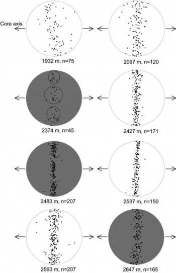
Fig. 5. Vertical view of the distribution of a-axis orientations measured on vertical thin sections. The arrows show the orientation of the core axis. The grey diagrams have anisotropic distributions.

Fig. 6. Explanation of distribution of a axes. (a) The c-axis orientation distribution which is generated artificially. (b) Random distribution of azimuth of a axes. (c) Schematic illustration of random orientation of a axes. (d) Schematic illustration shows a axes are aligned.
The constant-load uniaxial compression test is performed on the 2593 m sample at –15˚C. The goal of this test is to investigate the ice fabric evolution process during a uniaxial compression test. The thin-section photograph at 19% strain is shown in Figure 7. The original grain-size is 2.4 mm. Some grain boundaries cannot be recognized in some domains of the thin section by visual observation just under the crossed polarizer. It seems to change to ice single crystal. Although the degree of parallelism of the distribution of c-axis orientations increases from R = 93% to R = 97% after deformation, the azimuth distribution of the a axes in the whole section after the deformation does not drastically change from that before deformation (Fig. 8). However, there is some variation in the distribution of misorientation angle between adjacent grains. The misorientation angle, 9 , of the a axis between adjacent grains is defined as the average angle between three pairs of a axes. It is calculated as the angle between the a1 (or a 2, a 3) axis of grain A and the a1 (or a2, a3) axis of grain B. Each pair (a 1–a 1 , a2–a2, a 3–a3) lay in the same quadrant. The value of 9 will be in the range 0-60˚. Figure 9 shows a histogram of the frequency of the misorientation angle between grain pairs. The frequency of angles between adjacent grains after deformation (Fig. 9b) is significantly higher at low angles (2-8˚) than the frequencies both before deformation (Fig. 9a) and for the random pairing of grains (Fig. 9c). Figure 10 shows the a-axis orientation of adjacent grains in a given domain. There are three maxima in a-axis orientation in both domains. Some adjacent grains have almost the same a-axis orientation. Although it looks like a random distribution when all measured a axes are plotted (Fig. 8), the a-axis orientations are aligned in some domains. For adjacent grains before deformation (Fig. 9a), some frequencies of high angle (exceeding 40˚) appear. This means that, even in a given domain, the angular difference between adjacent grains has a large value before deformation.

Fig. 7. Photography of a vertical thin section from 2593m depth after deformation at 19% strain.

Fig. 8. Distribution of a-axis orientations after a constant-load compression test. The arrow indicates the compression axis.

Fig. 9. Histograms of the misorientation angle between grain pairs. The frequency of the misorientation angle within each 2˚ interval is shown. (a) Adjacent grains before deformation. (b) Adjacent grains after deformation. (c) Random pairs of grains after deformation.

Fig. 10. a-axis orientations of adjacent grains in a given domain. Each symbol represents one grain. Each grain has an adjoining relation in each domain.
We now propose an explanation of these distributions of a-axis orientations by using the anisotropy of crystallographic slip directions of ice single crystal across the basal plane. Some modeling (e.g. Reference Castelnau, Thorsteinsson, Kipfstuhl, Duval and CanovaCastelnau and others, 1996) includes the slip system on prismatic and pyramidal planes. If a slip system on a prismatic and/or pyramidal plane is active, it is thought that a axes gradually concentrate with depth. In the deep part of the GRIP ice core (i.e. strong single-maximum region of c axis), the concentration of a axis is observed partially with depth. We suggest that anisotropic distribution of a axes is attributable to local simple shear parallel to the horizontal direction of the ice sheet. Reference SteinemannSteinemann (1954) showed that the ice single crystal shear velocity parallel to [1120] is larger than the velocity parallel to [1010]. However, Steinemann concluded that there is no definite crystallographic slip direction in the basal plane. Reference KambKamb (1961) concluded that there is no preferred glide direction in the basal plane. Kamb also discussed experimental uncertainties. The experimental result about preferred glide direction in the basal plane is unclear due to experimental uncertainties. S. Mae (personal communication, 2003) indicated that the creep rate parallel to [1120] differs from the parallel to [1010] experimentally, but data with sufficient detail have not yet been published. There is no clear evidence about anisotropy of crystallographic slip direction of ice single crystal in the basal plane; however, if there is a preferred glide direction in the basal plane, the a axis of each grain will align to the simple shear direction under the condition in which the shear direction is perpendicular to the c axis (i.e. concentration axis of strong single maximum). Here, we assumed that easy-glide direction is parallel to [1120] in the basal plane. It is thought that a grain rotates so that the simple shear direction and [1120] become parallel and, as a result of this, the anisotropic distribution of a axes should be formed. It is unlikely that the GRIP drill site located at the dome summit region has undergone a large shear deformation; however, the ice-divide position may have moved in the past (e.g. Reference Anandakrishnan, Alley and WaddingtonAnandakrishnan and others, 1994). Such an anisotropic distribution of a axes in the GRIP ice core suggests that it is possible that the bottom part of the ice sheet has undergone a shear deformation frequently even around the summit region. Furthermore, if there is some difference in ice-flow stiffness by simple shear deformation between random distribution and anisotropic distribution of a axes, we may be able to explain the surprisingly high flow-law parameter and some fluctuations in the flow-law parameter value for the deep parts of the GRIP ice core. Such a difference in stiffness will also affect the horizontal velocity in the deep part of the ice sheets. The above observations are preliminary findings about anisotropic distribution of a axes. To discuss more detailed processes, further measurements of a-axis orientation in various ice cores and mechanical tests (e.g. simple shear test on strong single-maximum fabric ice) are needed.
Conclusion
The development and use of a high-accuracy X-ray apparatus have shown that distribution of a-axis orientations in the GRIP ice core is anisotropic at some depths. We also use the results of long-term uniaxial compression tests and X-ray crystallographic analyses to discuss ice fabric evolution. We propose the following model of ice fabric evolution in ice core from a dome summit region: In the upper part of the ice sheet, c axes rotate towards the axis of vertical compression. Consequently, c-axis orientations develop a strong single-maximum fabric in deeper parts of the ice sheet. Moreover, if the ice mass is deformed by simple shear caused by ice-divide migration, anisotropic distribution of a-axis orientations is formed. This model may help us to a better understanding of ice-sheet structure and the history of ice-sheet deformation. It also leads to improved ice-sheet flow models that include finer details of ice fabric evolution.
Acknowledgements
This work was supported by a grant-in-aid for JSPS Fellows from the Japan Society for the Promotion of Science and Creative Scientific Research (No. 14GS0202) from the Japanese Ministry of Education, Science, Sports and Culture. We thank S. Nakatsubo of the Institute of Low Temperature Science, Hokkaido University, for technical assistance, including designing of the X-ray device. Thanks also to K. Osaka for advice on X-ray measurement. Comments by two anonymous reviewers and the scientific editor, D. Dahl-Jensen, helped to improve the present paper. We also thank all members of the Greenland Ice Core Project (GRIP), organized by the European Science Foundation, for their support of this work.


