


1. Introduction
Columnar vortices can be viewed as an idealization of the structure generated by horizontal shear in geophysical settings, for example, the vortex street forming behind an island in the atmosphere (see e.g. Potylitsin & Peltier Reference Potylitsin and Peltier1998; Spedding Reference Spedding2014). In density-stratified flow experiments, turbulence generation often involves external stirring with a set of vertical bars (e.g. Holford & Linden Reference Holford and Linden1999), leading to vortex columns with pronounced vertical vorticity (Praud, Fincham & Sommeria Reference Praud, Fincham and Sommeria2005), which may become unstable and lead to turbulence. Numerical simulations often adopt a similar approach for energy injection into a stratified flow system, where turbulence is sustained by forcing the vertically uniform vortical modes (e.g. Waite & Bartello Reference Waite and Bartello2004; Brethouwer et al. Reference Brethouwer, Billant, Lindborg and Chomaz2007; Howland, Taylor & Caulfield Reference Howland, Taylor and Caulfield2020). The instabilities of such vertically uniform vortical motions are considered to provide an important link in the downscale energy transfer within strongly stratified turbulent flows (Augier, Chomaz & Billant Reference Augier, Chomaz and Billant2012; Waite Reference Waite2013).
One particular route for this energy pathway from (large) horizontal scales characterizing columnar vortices to (small) vertical scales influenced by buoyancy is the zigzag instability, first discovered by Billant & Chomaz (Reference Billant and Chomaz2000a,Reference Billant and Chomazb,Reference Billant and Chomazc). A distinguishing feature of this instability is that the most unstable vertical wavelength scales with  $U_0/N$, while the corresponding growth rate scales with $U_0/L$. Here, $U_0$ and $L$ are the characteristic horizontal velocity and length scale, respectively, and $N$ is the buoyancy frequency. Billant and Chomaz demonstrated how a columnar vortex pair (or a dipole), initially uniform in the vertical direction, would undergo a sinusoidal deformation that self-amplifies and results in the vortex dipole's breakdown. Direct numerical simulations (DNS) studies of the zigzag instability have been focused on a pair of vortices (Otheguy, Chomaz & Billant Reference Otheguy, Chomaz and Billant2006; Deloncle, Billant & Chomaz Reference Deloncle, Billant and Chomaz2008; Waite & Smolarkiewicz Reference Waite and Smolarkiewicz2008; Augier & Billant Reference Augier and Billant2011; Augier et al. Reference Augier, Chomaz and Billant2012), with the notable exception of Deloncle, Billant & Chomaz (Reference Deloncle, Billant and Chomaz2011), who investigated an array of vortices where the spacing between the vortices is much larger than the vortex size.
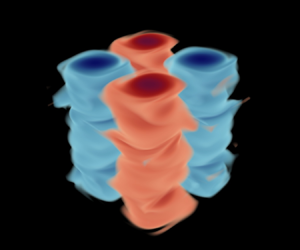
In the present study, we focus on a configuration featuring a two-by-two array of columnar vortices. The base flow, which can be considered as a vertically uniform variant of the flow first investigated by Taylor & Green (Reference Taylor and Green1937), is visualized in figure 1. The stability properties of various types of columnar vortex arrays have been studied for density-stratified and/or rotating fluids (Dritschel & de la Torre Juárez Reference Dritschel and de la Torre Juárez1996; Potylitsin & Peltier Reference Potylitsin and Peltier1998; Deloncle et al. Reference Deloncle, Billant and Chomaz2011; Suzuki, Hirota & Hattori Reference Suzuki, Hirota and Hattori2018; Hattori et al. Reference Hattori, Suzuki, Hirota and Khandelwal2021; Hattori & Hirota Reference Hattori and Hirota2023). Suzuki et al. (Reference Suzuki, Hirota and Hattori2018) considered two-dimensional (2-D) Taylor–Green (TG) vortices under stable stratification, highlighting the role of hyperbolic stagnation points in the instabilities of vortex arrays. They introduced a class of instabilities termed ‘strato-hyperbolic’ (SH), resulting from the interaction of hyperbolic instabilities in non-stratified TG vortices (see e.g. Leblanc & Godeferd Reference Leblanc and Godeferd1999) with internal gravity waves being phase-shifted near the hyperbolic stagnation points. More recently, Hattori et al. (Reference Hattori, Suzuki, Hirota and Khandelwal2021) identified additional instability types within the TG vortex array, including a novel ‘mixed hyperbolic’ (MH) instability. Hattori & Hirota (Reference Hattori and Hirota2023) further incorporated the effects of rotation in their stability analysis.

Figure 1. Visualization of columnar Taylor–Green vortices, i.e. the base flow described by (2.7). Colour illustrates the vertical vorticity  $\varOmega _z\equiv \partial _x V - \partial _y U$.
Despite being considered a generic mechanism (Billant & Chomaz Reference Billant and Chomaz2000c), the zigzag instability has yet to be identified in the context of a columnar vortex array, except in cases where the vortices are well separated from each other (Deloncle et al. Reference Deloncle, Billant and Chomaz2011). Suzuki et al. (Reference Suzuki, Hirota and Hattori2018) made a comparison between the zigzag and SH instabilities, describing the latter as a ‘short-wave’ instability for which the vertical wavelength and the horizontal scale of the vortices are comparable. In contrast, the zigzag instability was considered by Suzuki et al. (Reference Suzuki, Hirota and Hattori2018) as a ‘long-wave’ instability with wavelengths larger than the size of the vortices, although the authors also stated that this wavelength could decrease with strong stratification. Our paper will demonstrate that the instabilities in a columnar vortex array can indeed be short-wave. Hattori & Hirota (Reference Hattori and Hirota2023) contrasted the instabilities observed in TG vortices with those in the vortex array scenario investigated by Deloncle et al. (Reference Deloncle, Billant and Chomaz2011), noting that zigzag instability is more likely in the latter configuration due to the relatively large spacing between the vortices. They suggest that the absence of zigzag instability in TG vortices could be attributed to the ‘strong symmetry’ enforced by the periodicity over the horizontal plane.
When stratification is strong, i.e. when the Froude number ( $Fr$) is order 1 or below, Hattori et al. (Reference Hattori, Suzuki, Hirota and Khandelwal2021) showed that the MH instability tends to produce the most unstable mode across all vertical wavenumbers. The MH modes were shown to have vortical structures that are different from the SH modes. The fastest-growing wavenumber in MH modes, $k_{fgm}$, is smaller than in SH modes, and $k_{fgm}$ increases as $Fr$ decreases for MH modes, which is reminiscent of the scaling expected of zigzag instabilities. Hattori et al. (Reference Hattori, Suzuki, Hirota and Khandelwal2021) did not describe the physical mechanism associated with the growth of MH modes. The possible connection between MH modes and zigzag instability also remains unclear. To our knowledge, there have been no detailed studies of the MH modes beyond the linear stability analysis by Hattori et al. (Reference Hattori, Suzuki, Hirota and Khandelwal2021), and their exact role in the breakdown of columnar vortex arrays warrants further investigation.
In this paper, we examine the stability properties of columnar TG vortices using both linear stability analysis and DNS, with the main aim of understanding the primary instability of such a vortex array. We focus on  $Fr\leq 1$, for which the stratification is strong enough such that the most unstable wavelength of the primary instability, as we will show, follows the buoyancy scaling of $U_0/N$ (Billant & Chomaz Reference Billant and Chomaz2001). In § 2, we present the linear stability analysis, elucidate the instability mechanism of the unstable linear eigenmodes, and discuss connections with the zigzag instability. In § 3, we use fully nonlinear simulations to validate whether the linear instability identified in § 2 is indeed dynamically relevant in the breakdown of the TG vortices. Concluding remarks are offered in § 4.
2. Linear stability analysis
2.1. Formulation
The incompressible Navier–Stokes equations under the Boussinesq approximation are expressed in dimensional form as
 \begin{gather} {\frac{\partial{\boldsymbol{u}^*}}{\partial{t^*}}}+\boldsymbol{u}^*\boldsymbol{\cdot} \boldsymbol{\nabla}^* \boldsymbol{u}^* ={-}\frac{1}{\rho_0}\,\boldsymbol{\nabla}^* \varPi^* +\nu\,\nabla^{*2} \boldsymbol{u}^* +\frac{\rho^*}{\rho_0}\, \boldsymbol{g}, \end{gather}
 \begin{gather}\boldsymbol{\nabla}^* \boldsymbol{\cdot} \boldsymbol{u}^* =0. \end{gather}
Here,  $\boldsymbol {u}^*$ is the velocity field, $\rho _0$ is the reference density, $\nu$ is the kinematic viscosity, $\boldsymbol {g}=-g\hat {\boldsymbol {k}}$ is the gravitational acceleration, and $\rho ^*$ and $\varPi ^*$ represent the density and pressure deviations from the background density profile and the hydrostatic pressure balance, respectively. The total density $\rho _{tot}$ is decomposed into
 \begin{equation} \rho_{tot}(\boldsymbol{x}^*,t^*)=\rho_0 +\rho^*_{b}(z^*) + \rho^*(\boldsymbol{x}^*,t^*), \end{equation}
where the background density  $\rho ^*_{b}$ varies only with $z^*$. In the present study, $\rho ^*_{b}$ decreases linearly with $z^*$, which leads to a uniform buoyancy frequency $N=\sqrt {-(g/\rho _0)(\mathrm {d}\rho ^*_{b}/\mathrm {d}z^*})$. The evolution of $\rho ^*$ follows the advection–diffusion equation,
 \begin{equation} {\frac{\partial{\rho^*}}{\partial{t^*}}} + \boldsymbol{\nabla}^* \boldsymbol{\cdot} (\rho^* \boldsymbol{u}^* ) + w^*\,\frac{\mathrm{d}\rho^*_b}{\mathrm{d}z^*} = \kappa\,\nabla^2 \rho^*, \end{equation}
where  $\kappa$ is the diffusivity of density.
By non-dimensionalizing (2.1) and (2.3) using a characteristic length scale  $L$, velocity scale $U_0$, and time scale $L/U_0$, and rescaling $\rho ^*$ and $\varPi ^*$ as
 \begin{equation} \rho^* \sim \frac{N^2 L}{g}\,\rho_0,\quad \varPi^*\sim \rho_0 U_0^2, \end{equation}
respectively, we obtain the dimensionless governing equations
 \begin{gather} {\frac{\partial{\boldsymbol{u}}}{\partial{t}}} +\boldsymbol{u} \boldsymbol{\cdot} \boldsymbol{\nabla u} ={-}\boldsymbol{\nabla} \varPi +Re^{{-}1}\,\nabla^2 \boldsymbol{u} - Fr^{{-}2}\,\rho \hat{\boldsymbol{k}}, \end{gather}
 \begin{gather}\boldsymbol{\nabla} \boldsymbol{\cdot} \boldsymbol{u} =0, \end{gather}
 \begin{gather}{\frac{\partial{\rho}}{\partial{t}}} +\boldsymbol{u}\boldsymbol{\cdot} \boldsymbol{\nabla} \rho -w =(Re\,Pr)^{{-}1}\,\nabla^2\rho. \end{gather}
Here, the Reynolds, Froude and Prandtl numbers are
 \begin{equation} Re= \frac{U_0L}{\nu}, \quad Fr = \frac{U_0}{N L}, \quad Pr = \frac{\nu}{\kappa}, \end{equation}
respectively. In this paper,  $U_0$ is chosen such that dimensionless velocity in the base flow varies between $+1$ and $-1$, and $L$ is chosen such that the scaled wavelength of the base flow in the horizontal directions is $2{\rm \pi}$. In the remainder of this paper, we set $Re$ to 1600 and $Pr$ to 0.70, and focus on the effects of $Fr$ on the dynamics. The choice of $Re$ helps to keep the computational demands of DNS (§ 3) manageable.
We consider the 2-D base flow given by
 \begin{equation} (U, V, W) = (\sin x \cos y, -\cos x\sin y, 0), \end{equation}
for  $x,y\in [0,2{\rm \pi} )$ at $t=0$, which consists of an array of columnar vortices as illustrated in figure 1. The base flow is periodic in both horizontal directions, $x$ and $y$, and uniform in $z$. The pressure field $P_0$, streamfunction $\psi$, and vertical component of vorticity $\varOmega _z$ associated with the base flow are
 \begin{equation} P_0 = \tfrac{1}{4}(\cos 2x + \cos 2y), \quad \psi = \sin x \sin y, \quad \varOmega_z = 2\sin x \sin y, \end{equation}
respectively. The streamfunction and vorticity are related via  $\nabla ^2\psi =-\varOmega _z$. Incidentally, for this base flow, $\psi$ and $\varOmega _z$ have the same dependence on $x$ and $y$. Due to viscous effects, the base flow velocities ( $U$,
$U$,  $V$) and pressure ( $P_0$) would decay as $\exp (-2t/Re)$ and $\exp (-4t/Re)$, respectively (see e.g. Kim & Moin Reference Kim and Moin1985), in the absence of flow instabilities. Our linear stability analysis detailed below, however, will focus on the base flow at $t=0$, disregarding its considerably slow decay ( $Re\gg 1$) due to viscosity.
We seek infinitesimal, three-dimensional (3-D) perturbations to the base flow that are expressed in normal modes in the  $z$-direction:
 \begin{equation} (u', v', w', \rho', p') = (\hat{u}, \hat{v}, \hat{w}, \hat{\rho}, \hat{p}) \exp (\mathrm{i}kz +\sigma t)+\textrm{c.c.},\end{equation}
where the  $\hat {\cdot }$ quantities vary in $(x,y)$. For simplicity, all primes on the perturbation variables will be dropped for the remainder of this paper. Linearizing the governing equations (2.5) for the base flow (2.7) yields the generalized eigenvalue problem
 \begin{equation} \sigma \begin{bmatrix} \boldsymbol{\varDelta} & & \\ & \boldsymbol{\varDelta} & \\ & & \boldsymbol{I} \end{bmatrix} \begin{bmatrix} \hat{u} \\ \hat{v} \\ \hat{\rho} \end{bmatrix}= \begin{bmatrix} \boldsymbol{L}_{uu} & \boldsymbol{L}_{uv} & \boldsymbol{L}_{u\rho}\\ \boldsymbol{L}_{vu} & \boldsymbol{L}_{vv} & \boldsymbol{L}_{v\rho}\\ \boldsymbol{L}_{\rho u} & \boldsymbol{L}_{\rho v} & \boldsymbol{L}_{\rho \rho} \end{bmatrix} \begin{bmatrix} \hat{u} \\ \hat{v} \\ \hat{\rho} \end{bmatrix}, \end{equation}
where  $\boldsymbol {I}$ is an identity matrix, and the other linear operators are as follows:
 \begin{align} \varDelta &=\partial_{xx} + \partial_{yy} -k^2, \end{align}
 \begin{align} \boldsymbol{L}_{uu} &= (-\varDelta +\partial_{xx})(U\,\partial_x+V\,\partial_y+\partial_x U)+\partial_{xy}(\partial_xV)\nonumber\\ &\quad -\partial_x(U\,\partial_x+V\,\partial_y)\,\partial_x+Re^{{-}1}\,\varDelta^2, \end{align}
 \begin{align} \boldsymbol{L}_{uv}&=(-\varDelta +\partial_{xx})\,\partial_yU+\partial_{xy}(\partial_yV+U\,\partial_x+V\,\partial_y)\nonumber\\ &\quad -\partial_x(U\,\partial_x+V\,\partial_y)\,\partial_y, \end{align}
 \begin{align} \boldsymbol{L}_{u\rho}&=Fr^{{-}2}\,(\mathrm{i}k)\,\partial_x, \end{align}
 \begin{align} \boldsymbol{L}_{vu}&=(-\varDelta +\partial_{yy})\,\partial_xV+\partial_{yx}(\partial_xU+U\,\partial_x +V\,\partial_y)\nonumber\\ &\quad -\partial_y(U\,\partial_x+V\,\partial_y)\,\partial_x, \end{align}
 \begin{align} \boldsymbol{L}_{vv}&=(-\varDelta+\partial_{yy})(U\,\partial_x+V\,\partial_y+ \partial_yV)+\partial_{xy}(\partial_yU)\nonumber\\ &\quad -\partial_y(U\,\partial_x+V\,\partial_y)\,\partial_y+Re^{{-}1}\,\varDelta^2, \end{align}
 \begin{align} \boldsymbol{L}_{v\rho}&=Fr^{{-}2}\,(\mathrm{i}k)\,\partial_y, \end{align}
 \begin{align} \boldsymbol{L}_{\rho u}&={-}({\mathrm{i}k})^{{-}1}\,\partial_x, \end{align}
 \begin{align} \boldsymbol{L}_{\rho v}&={-}({\mathrm{i}k})^{{-}1}\,\partial_y, \end{align}
 \begin{align} \boldsymbol{L}_{\rho\rho}&={-}(U\,\partial_x+V\,\partial_y)+(Re\,Pr)^{{-}1}\varDelta. \end{align}
The full derivation of this linear system is given in Appendix A. A formulation similar to the present one to identify 3-D perturbations in a 2-D base flow (thus referred to as ‘2B3P’) was used successfully to analyse experimental data from a stratified inclined duct (Chomaz Reference Chomaz2018; Lefauve et al. Reference Lefauve, Partridge, Zhou, Dalziel, Caulfield and Linden2018). The eigenvalue problem (2.10) is solved numerically using the MATLAB eig function. The differential operators along the periodic  $x$- and $y$-directions are discretized with the Fourier differentiation matrix (Weideman & Reddy Reference Weideman and Reddy2000), ensuring the horizontal periodicity of the resulting eigenmodes. The size of the eigenvalue problem is considerably large: using $\hat {N}$ Fourier points to discretize one horizontal direction results in two matrices of size $3\hat {N}^2$ by $3\hat {N}^2$ in (2.10). We used $\hat {N}=64$ and $72$ to solve the linear system, which produced nearly identical physical eigenvalues and eigenmodes between the two $\hat {N}$ values. Unphysical, spurious eigenmodes may arise, which are identifiable through a comparison of results from the two $\hat {N}$ values tested.
2.2. Linear dispersion relation
Our investigation will focus on the effects of varying  $Fr$, specifically for $Fr\in \{1,1/2,1/4,1/8\}$. We selected this range of $Fr$ because, as we will demonstrate, the fastest-growing modes at these values exhibit zigzag-like properties. Billant & Chomaz (Reference Billant and Chomaz2000c) observed zigzag instabilities in vortex dipoles when $Fr < 0.2$. The apparent inconsistency in the $Fr$ ranges associated with zigzag instabilities arises from the difference in the choices of velocity and length scales used to define $Fr$. This distinction is also crucial for comparing dimensional quantities across different set-ups, as we discuss later in this subsection. We will report DNS conducted in a triply periodic domain for these $Fr$ values in § 3. For linear stability analysis, we vary the vertical wavenumber $k$ within the range 1–20 (integers only) due to the constraint that only integer modes of $k$ are permissible in the DNS for domain height $2{\rm \pi}$. We display the solution branch that produces the fastest-growing mode across all wavenumbers for each $Fr$ in figure 2. For this specific branch of eigenmodes, the imaginary part of $\sigma$ is zero, i.e. $\sigma _i\equiv {\rm Im}({\sigma })=0$, suggesting that all these modes are stationary. Another solution branch (not shown in figure 2) that emerges from the stability analysis corresponds to the pure hyperbolic (PH) mode that was investigated by Hattori et al. (Reference Hattori, Suzuki, Hirota and Khandelwal2021). The PH modes can be easily distinguished from the solution branch shown in figure 2 as the PH modes have a non-zero frequency ( $\sigma _i\neq 0$). The instability mechanism of the PH mode does not require stratification (Leblanc & Godeferd Reference Leblanc and Godeferd1999), and the most unstable mode occurs at $k=0$, i.e. when the perturbation structure is 2-D.

Figure 2. Growth rate  $\sigma _r$ plotted against (a) $k$ and (b) $k\,Fr$ for the solution branch containing the fastest-growing mode: $\Diamond$, $Fr=1.0$; ${\bigtriangleup}$, $Fr=0.5$; $\ast$, $Fr=0.25$; $\Box$, $Fr=0.125$.
Figure 2 demonstrates that the growth rate  $\sigma _r\equiv {\rm Re}({\sigma })$ initially increases with $k$ for smaller values of $k$, and subsequently decreases as $k$ increases further. The fastest-growing $k$ (table 1) shifts to the left as $Fr$ increases. When $k$ is adjusted by multiplying it by $Fr$, the increasing flank of the curves nearly collapses, and the peak growth rate occurs within a narrow range of $k\,Fr$ between 1.1 and 2.0, i.e. for the most unstable mode,
 \begin{equation} k\sim Fr^{{-}1}.\end{equation}
Or, in dimensional form, the fastest-growing wavelength  $\lambda ^{*}_z\equiv (2{\rm \pi} /k)L$ scales as
 \begin{equation} \lambda^{*}_z\sim (2{\rm \pi})(U_0/N).\end{equation}
The maximum non-dimensional growth rates  $\sigma$, summarized in table 1, exhibit no significant variability with respect to $Fr$. Accordingly, the dimensional growth rate $\sigma ^{*}\equiv \sigma U_0/L$ scales as
 \begin{equation} \sigma^{*}\sim U_0/L.\end{equation}
Table 1. The most unstable mode at each  $Fr$ considered.

In their examination of zigzag instability, Billant & Chomaz (Reference Billant and Chomaz2000b) (hereafter referred to as BC00) observed that the vertical scale most susceptible to zigzag instability in a vortex pair scales with  $U_0/N$, i.e. (2.13), and the maximum growth rate with $U_0/L$, i.e. (2.14). These scalings are markedly similar to the results presented above for the vortex array. The scaling (2.12) is in contrast to the elliptic instability for which the fastest-growing wavenumber and growth rate both increase with $Fr$ (see e.g. figure 2 of Billant & Chomaz Reference Billant and Chomaz2000c). Figure 2 presents dispersion relations that are at least qualitatively similar to those identified by BC00 (see e.g. their figure 7), i.e. the growth rate $\sigma _r$ peaks at a non-zero vertical wavenumber $k$. This contrasts with horizontally sheared flows, which feature a one-dimensional velocity profile varying along the horizontal direction with gravity oriented in the spanwise direction (Deloncle, Chomaz & Billant Reference Deloncle, Chomaz and Billant2007; Arobone & Sarkar Reference Arobone and Sarkar2012; Lucas, Caulfield & Kerswell Reference Lucas, Caulfield and Kerswell2017). In such flows, the most unstable modes have a zero vertical wavenumber, an observation considered by Deloncle et al. (Reference Deloncle, Chomaz and Billant2007) as an extension of Squire's theorem to stratified flows.
Additionally, the primary instability of a TG vortex array resembles the zigzag instability observed in vortex dipoles in several key aspects. For both cases, the eigenvalues for the fastest-growing modes are real ( $\sigma _i = 0$), and the dispersion relation reveals an approximately linear relationship between the dimensionless growth rate ( $\sigma _r$) and small values of $k\,Fr$, as shown in figure 9 of Billant & Chomaz (Reference Billant and Chomaz2000c). Data for the vortex array included in figure 2(b) suggest a linear relation (not shown) between $\sigma _r$ and $k\,Fr$, which collapses data across various $Fr$ values between 0.125 and 0.5 for $k\,Fr\lesssim 1$. Furthermore, the magnitude of the peak growth rates, when dimensionalized, lies between 0.20 and 0.24 times $U_0/L$, or 0.63–0.75 times $U_0/D$, where $D = {\rm \pi}L$ represents the distance between the centres of two adjacent oppositely signed vortices (figure 1). Using similar metrics, the dimensional growth rate $\sigma ^*$ typically ranges from 0.6 to 0.7 times $U_0/D$ in the dipole scenario, according to figure 9 of Billant & Chomaz (Reference Billant and Chomaz2000c), where $D\approx L$ following figure 1 of BC00.
As discussed earlier, our study focuses on the range  $0.125 \leq Fr \leq 1$, where the primary instability exhibits many characteristics similar to the zigzag instability. For $Fr$ values outside this range, the PH mode (Hattori et al. Reference Hattori, Suzuki, Hirota and Khandelwal2021) shows a higher growth rate across all wavenumbers. Specifically, for $Fr < 0.125$, the dispersion relation of the zigzag modes at $Fr=0.0625$ (not shown) exhibits a reduced maximum growth rate, and the latter is also lower than that of the PH mode at this $Fr$. For larger $Fr$ values, figure 8 of Hattori et al. (Reference Hattori, Suzuki, Hirota and Khandelwal2021) indicates that the PH mode becomes the dominant instability for $Fr > {\rm \pi}$, surpassing the zigzag modes. Currently, we do not have sufficient data to pinpoint the exact transition point in terms of $Fr$ between zigzag and PH modes, and this critical $Fr$ value might also vary with $Re$. Nonetheless, the evidence available seems to suggest that this transitional $Fr$ is likely to be greater than 1 and probably of $O(1)$. In summary, within the $Fr$ range $O(0.1)$ to $O(1)$, the zigzag mode, whose most unstable eigenmode appears to be 3-D ( $k\neq 0$), tends to dominate. Outside this $Fr$ range, the fastest-growing instability shifts to the 2-D PH modes ( $k=0$), whose instability mechanism does not rely on stratification.
2.3. Instability mechanism
We now turn our attention to the most unstable eigenmode at  $k=3$ for $Fr=0.5$, using it as an example to shed light on the underlying instability mechanism. The characteristics of the 2-D base flow are illustrated in figure 3, while the horizontal structure of the 3-D eigenmode is displayed in figure 4. In particular, figure 4(a), which shows the vertical vorticity perturbation $\omega _z\equiv \partial _x v - \partial _y u$, reveals horizontal structures similar to those presented in figure 5 of Hattori et al. (Reference Hattori, Suzuki, Hirota and Khandelwal2021) (hereafter referred to as H21). These structures are identified by H21 as MH modes. In line with our results in § 2.2, H21 demonstrated that the MH modes, specifically the branch with $\sigma _i=0$, yield the highest growth rate $\sigma _r$ for their cases with $Fr\leq {\rm \pi}/2$ (equivalently, $F_h\leq 0.5$ in the H21 terminology, with $F_h\equiv Fr/{\rm \pi}$ due to the differences in the definitions). Furthermore, H21 noted an increase in the fastest-growing $k$ as $Fr$ decreased from $0.2{\rm \pi}$ to $0.1{\rm \pi}$, consistent with the expected behaviour for zigzag instabilities.

Figure 3. Base flow characteristics: (a) vorticity  $\varOmega _z$, (b) streamfunction $\psi$, and (c) pressure $P_0$. The dashed line in (a) marks the line $y=x$, along which a vertical transect is illustrated in figure 5. The contours of $\psi$ are shown in (b) for $0.125\leq |\psi |\leq 0.875$, with an interval of $0.125$ between adjacent contour levels. The symbol ${\bigtriangleup}$ in (b) indicates the location of an elliptical stagnation point, and $\Box$ indicates a hyperbolic stagnation point.

Figure 4. Horizontal transect of perturbation (a)  $\omega _z$ at $z=z_0$, (b) $\rho$ at $z=z_+$, and (c) $w$ at $z=z_+$, for the eigenmode with $k=3$ at $Fr=0.5$. The heights $z_0$ and $z_+$ are specified in figure 5. The amplitude of the eigenmode is normalized such that the kinetic energy associated with the horizontal perturbation velocities $(u,v)$ constitutes $1\,\%$ of the kinetic energy in the base flow $(U,V)$. The dashed line indicates the streamline corresponding to $\psi =0.25$, and the solid dot indicates the starting point of a particle trajectory considered in figure 6.
H21 classified these MH modes as a subtype of hyperbolic instabilities, alongside PH modes, which are independent of stratification, and SH modes, which result from the phase shifts in internal gravity waves induced by PH modes. The ‘mixed’ nature of these modes arises, according to H21, from the vorticity distribution being a combination of both PH and SH instabilities. H21 did not describe the physical mechanism of MH modes in detail. Here, we will take a different perspective and elucidate how the MH modes become unstable by drawing parallels to the zigzag instabilities in the vortex dipole case studied by BC00.
To start, it is useful to summarize the zigzag instability mechanism for dipoles as outlined by BC00. The mechanism begins with an initial pressure distribution  $P_0$ associated with the base flow. A height-varying horizontal displacement of the dipole column induces a vertical pressure gradient, leading to isopycnal deformation (as shown in their figure 3a) due to the hydrostatic balance between the density perturbation $\rho$ and pressure perturbation $p$. This mechanism, which was also considered by Basak & Sarkar (Reference Basak and Sarkar2006), is described by the linearized vertical momentum equation (A1c) in hydrostatic balance, i.e.
 \begin{equation} {- \partial_z p} \approx Fr^{{-}2}\,\rho.\end{equation}
The displacement of isopycnals due to  $\rho$ initiates a vertical velocity $w$ as per the linearized density equation (A6), assuming negligible diffusion,
 \begin{equation} \partial_t\rho + (U\,\partial_x + V\,\partial_y)\rho \approx w,\end{equation}
where the right-hand side arises due to the perturbation vertical velocity  $w$, and the non-dimensional background density gradient $\mathrm {d}\rho _b/\mathrm {d}z=-1$. The linear equation (A6) indicates that a fluid parcel, while being transported by the base flow $(U,V)$, undergoes density fluctuations directly coupled to vertical velocity $w$. A distinct feature of the zigzag instability is its stationarity, i.e. $\sigma _i=0$, as discussed in § 2.2. As a result, the motion of a fluid parcel undergoing zigzag instability can be seen as traversing a loop that samples a stationary, horizontal pattern of the flow (see figure 3(a) of BC00), rather than linear oscillation around an equilibrium position as in an internal wave ( $\sigma _i\neq 0$). This vertical motion induced by this mechanism causes straining in the vertical direction, i.e. $\partial _z w\neq 0$, leading to diverging horizontal perturbation velocities ( $\partial _x u+\partial _y v\neq 0$). The horizontal perturbation velocities $(u,v)$ further displace the dipole horizontally and introduce rotational ‘twists’ within the dipole, thus amplifying the initial perturbations and completing the feedback loop that characterizes the zigzag instability mechanism.
Some key features of the TG base flow are revisited in figure 3 in light of the zigzag mechanism. The TG base flow vorticity  $\varOmega _z$ (figure 3a) and streamfunction $\psi$ (figure 3b) have the same structure over the $x$–
$x$– $y$ plane, which means that a fluid parcel advected by the base flow would encounter a constant $\varOmega _z$ along a streamline. Two types of stagnation points exist (figure 3b): elliptical and hyperbolic. Figure 3(c) demonstrates that the base flow pressure $P_0$ attains its highest values at the hyperbolic stagnation points, and lowest at the elliptical stagnation points.
To leading order, the perturbations to the vortex dipole analysed by BC00 involve a simple horizontal translation of the vortical structure, resulting in a sinusoidal deformation of the vortex column, as illustrated in their figure 3. In the TG case, the  $\omega _z$ perturbations displayed in figure 4(a) reveal more complex spatial variations than would be expected from a mere horizontal translation of columnar vortices. The vertical–horizontal transects presented in figure 5 demonstrate how the base flow $\varOmega _z$ in figure 5(a) is modified by the perturbation $\omega _z$ in figure 5(b) to form the ‘bent’ pattern in figure 5(c), similar to the dipole scenario. Figure 5(b) suggests that large magnitudes of $\omega _z$ are located at the ‘edges’ of the vortex column, leading to pronounced bending at these locations – for instance, see the contour of the perturbed vorticity $\varOmega _z+\omega _z$, at 0.2 in figure 5(c). Conversely, the magnitude of $\omega _z$ near the centre of the columns is relatively small, resulting in less pronounced bending and in a direction opposite to that at the edges, as shown by the $\varOmega _z+\omega _z$ contour at 1.8 in figure 5(c). Strictly speaking, the zigzag instability involves only a displacement of the vortex core as a whole. The vortex structure depicted here also shows an internal deformation of the vortex, which might seem closer to the elliptic instability in appearance (see e.g. figure 4 of Otheguy et al. Reference Otheguy, Chomaz and Billant2006). However, it will be demonstrated in the following that the instability mechanism is indeed ‘zigzag-like’.

Figure 5. Vertical–horizontal transect of (a) base flow  $\varOmega _z$, (b) perturbation $\omega _z$, (c) $\varOmega _z+\omega _z$, and (d) vertical velocity $w$. The horizontal axis $x'$ represents the distance from the origin along the line $y=x$, indicated by a white dashed line in figure 3. One full vertical wavelength is shown in $z$. Dotted lines in (a) and (c) display vertical vorticity contours at 0.2 and 1.8, respectively. Symbols ${\bigtriangleup}$ and ${\bigtriangledown}$ mark the heights $z_+$ and $z_-$, respectively, where $w$ attains its maximum magnitude, and $\circ$ is the height $z_0=(z_++z_-)/2$, where $\omega _z$ reaches the maximum magnitude.
Following the BC00 argument, the deformation of the vortex columns (figure 5c) produces a horizontal shift of the associated pressure field  $P_0$ (figure 3c). This shift results in a $z$-dependent pressure field ( $\partial _z p\neq 0$), which is associated with density perturbations $\rho$ (figure 4b) through the hydrostatic balance (2.15). The $\rho$ perturbation is then associated with vertical velocities $w$ (figure 4c) via (2.16). The vertical structures of such $w$ perturbations are presented in figure 5(d). Consistent with figure 3(b) of BC00, figure 5(d) demonstrates that $w$ vanishes at $z=z_0$ where $|\omega _z|$ reaches maximum, i.e. where the vortex column experiences the greatest horizontal displacement. The magnitude of $w$ peaks a quarter vertical wavelength away from $z_0$ at $z_+$ or $z_-$, coinciding with the heights at which $|\omega _z|$ is at its lowest.
The connection between the  $\rho$ and $w$ perturbations, shown in figures 4(b) and 4(c), respectively, becomes clear when considering (2.16) within the scenario of a fluid parcel moving with the base flow. We focus on a particular streamline, marked by a dashed line in figure 4, and examine perturbations along this streamline at various heights as shown in figure 6. In terms of the $\omega _z$ perturbation, as discussed previously, its magnitude reaches the maximum at $z=z_0$, and nearly vanishes at $z=z_+$ and $z_-$. In contrast, the perturbations $\rho$ and $w$ exhibit significant magnitudes at $z=z_+$ and $z_-$, where both quantities are of the same magnitude but oppositely signed at $z=z_+$ and $z_-$, respectively, for any given point along the streamline, reflecting the anti-symmetry about the height $z=z_0$. The rate of change of $\rho$ with respect to the distance ( $s$) along the streamline, $\partial _s \rho$, a proxy for the left-hand side of (2.16), is closely associated with $w$, as evidenced by figure 6. For example, $\partial _s \rho > 0$ tends to coincide with $w>0$, and vice versa. This confirms that $\rho$ and $w$ are coupled via (2.16) at a given height of the columnar vortex, highlighting a key element in the zigzag mechanism.

Figure 6. Profiles of perturbation  $\omega _z$, $\rho$ and $w$ along a specific base flow streamline ( $\psi =0.25$) at various heights: (a) $z=z_+$, (b) $z=z_{0}$ and (c) $z=z_{-}$. This particular streamline is marked in figure 4 with a white dashed line. The profiles commence at the location indicated by a solid dot in figure 4, and trace the $\psi$ contour in the anticlockwise direction, following the path of a fluid parcel moving according to the base flow $(U,V)$.
With isopycnal deformations inducing  $z$-dependent $w$ perturbations, $\partial _z w$ becomes non-zero, balanced by non-zero $\partial _x u + \partial _y v$ in the continuity equation. Figure 7(a) shows the flow pattern over an $x$–
$x$– $y$ plane, where the $(u,v)$ velocities typically originate from regions of vertical convergence ( $\partial _z w<0$) and move towards regions of divergence ( $\partial _z w>0$) to maintain continuity. This complex flow pattern results in the formation of vortical structures (figure 7b), including a pair of vortices with opposite signs near the hyperbolic stagnation point at $(x,y) = ({\rm \pi},{\rm \pi} )$. Such vortical perturbations, manifested as $\omega _z$, complete the dynamical feedback loop initiated by the deformation of the columnar vortices (figure 4a). As a result, the instability is expected to grow, following the dynamics outlined above, which closely resemble those of the zigzag instability proposed by BC00.

Figure 7. Horizontal velocity vector field  $(u,v)$ visualized by arrows, overlaid by colour maps showing (a) $\omega _z$, and (b) $\partial _z w$, at $z=z_0$.
3. Direct numerical simulations
3.1. Numerical configuration
To examine the nonlinear evolution of the unstable modes identified in § 2 and their role in the breakdown of columnar TG vortices into turbulence, we conducted DNS using the lattice Boltzmann (LB) method. The LB flow solver, known as ‘OpenLB’, was developed by Krause et al. (Reference Krause2020) and has been adapted to solve the Boussinesq-approximated Navier–Stokes equations (2.5) by Guo, Zhou & Wong (Reference Guo, Zhou and Wong2023) for wall-bounded stratified turbulent flows. An overview of the LB solver is provided in Appendix B. Additionally, we performed further validation of this LB solver against pseudo-spectral DNS in a triply periodic configuration, an effort that is also documented in Appendix B.
We carried out four simulations of the columnar TG flow within a triply periodic domain of length  $2{\rm \pi}$ in each direction, employing the same parameters examined in § 2. The specifics of these simulations are detailed in table 2. The computational mesh is uniform and isotropic. The grid spacing is no more than twice the Kolmogorov scale during peak dissipation. The simulations were initiated with the base flow defined by (2.7) at $t=0$, with the phases of the sinusoidal functions slightly altered by random noise. Specifically, the initial conditions were set as
 \begin{equation} (U, V, W) = [\sin (x+\epsilon_1) \cos (y+\epsilon_2), -\cos (x+\epsilon_3)\sin (y+\epsilon_4), 0 + \sin(\epsilon_5)],\end{equation}
where the phase shifts ( $\epsilon$) are computer-generated pseudo-random numbers uniformly distributed within the range $[-0.01, 0.01]$. This introduction of low-level noise is critical for symmetry breaking and triggering instabilities, as suggested by Riley & de Bruyn Kops (Reference Riley and de Bruyn Kops2003) in their study of the turbulence generated by the breakdown of 3-D TG vortices.
Table 2. Parameters of DNS for  $(Re,Pr)=(1600,0.7)$ and various Froude numbers. Here, $(N_x,N_y,N_z)$ are the number of lattice points used in each direction, $\Delta t$ is the time step size, $\bar {\sigma }$ is the estimated overall linear growth rate (§ 3.3), $k_{fgm}$ and $\lambda _{fgm}$ are the observed fastest-growing wavenumber and wavelength, respectively, and $\ell _v$ and $Fr_v$ are the vertical length scale (3.4) and Froude number (3.5), respectively, for the time when the perturbation kinetic energy $E_k$ in (3.3a,b) first exceeds 0.01.

3.2. Flow phenomenology
The evolution of the flow is visualized through volume-rendered colour images of vertical vorticity in figure 8 for the case  $Fr=0.5$. The sequence starts with an image at $t=32$, where the vortex structure is similar to the base flow (figure 1), with weak perturbations manifesting as corrugations on the surface of the vortex tube. By $t=40$ (top right image), these corrugations have intensified. Images in the middle row reveal the emergence of nonlinear dynamics, such as secondary perturbations between and then within the columns, which quickly evolve into turbulence for $44 \leq t \leq 52$. The bottom row illustrates the decay of turbulence from its maximum intensity. Figure 9 shows the corresponding sequence of images for $Fr=0.25$. Relative to the $Fr=0.5$ case, the corrugations on the vortex tube surface appear at a finer vertical length scale, and the transition to a fully disorganized state at $t=56$ (bottom left image) appears to occur more gradually as compared to the $Fr=0.5$ case.

Figure 8. Snapshots of the vertical vorticity field from the DNS with  $Fr=0.5$. The initial image in the sequence was captured at time $t=32$. Subsequent images are spaced at regular intervals of 4.0 units of time, arranged from left to right and top to bottom.

Figure 9. Same layout as figure 8 for the case with  $Fr=0.25$.
3.3. The energetics
The flow field can be decomposed into a vertically averaged component  $\bar {\boldsymbol U}=(\bar {U},\bar {V},0)$ and the fluctuation $\boldsymbol {u}=(u,v,w)$. The kinetic energy contained in the mean velocities can be quantified by
 \begin{equation} \bar{E}_k=\tfrac{1}{2} \langle \bar{\boldsymbol U} \boldsymbol{\cdot} \bar{\boldsymbol U}\rangle, \end{equation}
where  $\langle \cdot \rangle \equiv (2{\rm \pi} )^{-3}\iiint (\cdot )\, \mathrm {d}\kern0.7pt x\,\mathrm {d} y\,\mathrm {d}z$ denotes volume average over the entire domain. There is no mean potential energy associated with the density perturbation $\rho$. Note that $\bar {\boldsymbol U}$ in general differs from the base flow (2.7) due to viscous decay and flow instabilities. The kinetic energy and potential energy contained in the fluctuation field are
 \begin{equation} E_k = \frac{1}{2} \langle \boldsymbol u \boldsymbol{\cdot} \boldsymbol u \rangle, \quad E_p = \frac{1}{2\,Fr^2}\,\langle \rho^2 \rangle,\end{equation}
respectively.
We examine the energetics in the system through figure 10, taking the  $Fr=0.5$ and $0.25$ cases as an example. Figures 10(a,b) display energy on a linear scale, revealing that for a significant duration, up to $t\lesssim 40$ for $Fr=0.5$, and $t\lesssim 45$ for $Fr=0.25$, the kinetic energy is dominated by the vertically uniform (mean) component, $\bar {E}_k$. The mean kinetic energy slowly decays linearly due to viscosity at the anticipated rate $\exp (-4t/Re)$. Figures 10(c,d), where energy is plotted on a logarithmic scale, indicate that following the initial adjustments to the random noise, the fluctuation kinetic and potential energy ( $E_k$ and $E_p$, respectively) grow linearly with time, i.e. $E_k, E_p\propto \exp (2\bar {\sigma }t)$. The overall growth rates $\bar {\sigma }$, which do not vary significantly across all four $Fr$ cases, are tabulated in table 2. At $t\approx 40$ for $Fr=0.5$ and $t\approx 45$ for $Fr=0.25$, both $E_k$ and $E_p$ experience a significant upsurge as shown in the linear plots, alongside a rapid decline in the mean $\bar {E}_k$ as the flow transitions to turbulence. The fluctuation energies $E_k$ and $E_p$ depart from the linear trend and saturate by $t\approx 50$ for $Fr=0.5$, and by $t\approx 55$ for $Fr=0.25$, at which stage the mean energy component has been reduced significantly. Beyond this point, the fluctuating $E_k$ becomes the dominant form of kinetic energy and starts to decrease rapidly, along with the potential energy $E_p$.

Figure 10. Time series of various energy components, for (a,c)  $Fr=0.5$ and (b,d) $Fr=0.25$. Energy is plotted (a,b) on a linear scale, and (c,d) on a logarithmic scale.
The growth in the fluctuation energy is contributed by various vertical wavenumbers  $k$. In figure 11, we examine the vertical spectra of kinetic energy of $E_k$, denoted as $\tilde {E}_k$, as they vary with $k$ and over time for $Fr=0.5$. Figure 11(a) demonstrates the overall growth of kinetic energy across a range of vertical wavenumbers for $16\leq t \leq 40$, coinciding with the linear growth phase of the instabilities (see figure 10c). The linear growth is non-uniform across wavenumbers. By $t=24$, the mode of $k=3$ has surpassed all other modes in terms of the energy level. Incidentally, $k=3$ is also the fastest-growing mode predicted by the linear stability analysis (table 1); more discussion on this will follow in the next subsection. Figure 11(b) shows that each mode of different $k$ also follows its own rate of linear growth, $\sigma (k)$. Again, the mode with $k=3$ gains the most energy during the linear growth stage of the instabilities.

Figure 11. Sample fluctuation kinetic energy spectra for  $Fr=0.5$ displayed (a) as a function of $k$, and (b) as a function of $t$. For (a), the spectra are selected from $16\leq t \leq 40$, at intervals of 4.0 time units, with the curves shifting upwards as time progresses.
In figure 12, we investigate the vertical length scale  $\ell _v$, which characterizes the energy-containing scales in the initially uniform $z$-direction. Similar to Zhou & Diamessis (Reference Zhou and Diamessis2019), who used $\ell _v$ to characterize the vertical scale associated with spontaneously formed shear layers in stratified turbulent wakes, we define
 \begin{equation} \ell_{v}(t)\equiv2{\rm \pi} \left.\int_{ k_{min}}^{k_{nyq}} k^{{-}1}\,\tilde{E}_{k}(k,t)\,\textrm{d} k \right/ \int_{ k_{min}}^{k_{nyq}}\tilde{E}_{k}(k,t) \,\textrm{d}k, \end{equation}
where  $k_{min}=1.0$ is the minimum wavenumber, and $k_{nyq}$ is the Nyquist wavenumber ( $k_{nyq}$ is $126$ for $Fr\geq 0.5$, and $251$ for $Fr<0.5$). Figure 12 indicates that $\ell _v$ stays relatively constant over time after the initial transients, but exhibits a strong dependence on $Fr$. As $Fr$ decreases, the vertical length scale that emerges before the breakdown of columnar vortices also decreases, again reminiscent of the anticipated scaling of zigzag instabilities.


To examine whether the dimensional vertical length scale  $\ell _v^*\equiv \ell _vL$ follows the expected $U_0/N$ scaling, it is helpful to examine an inverse vertical Froude number,
 \begin{equation} Fr_v^{{-}1}=\frac{\ell_v^*N}{U_0}= \frac{\ell_v}{Fr}.\end{equation}
Characteristic values of  $Fr_v$ are tabulated in table 2, where they exhibit the same order of magnitude and a decreasing trend as $Fr$ decreases. This relationship between $Fr_v$ and $Fr$ is consistent with the results from forced DNS by Waite & Bartello (Reference Waite and Bartello2004) and Brethouwer et al. (Reference Brethouwer, Billant, Lindborg and Chomaz2007). In contrast, in the decaying turbulence simulations by Maffioli & Davidson (Reference Maffioli and Davidson2016), $Fr_v$ was observed to approach a relatively narrow range as the flow transitions towards relaminarization.
3.4. Comparison with linear stability analysis
In figures 13 and 14, we examine the flow structure in the DNS of  $Fr=0.5$, captured at $t=32$ during the linear growth stage of the instabilities (figure 10). Figure 13 displays the perturbation field over the $x$–
$x$– $y$ plane. The $\omega _z$ field is taken at the height ( $z_0$) where the $\omega _z$ magnitude is found to be at maximum, and $\rho$ and $w$ are shown at the height one-quarter vertical wavelength $\lambda _{fgm}\equiv 2{\rm \pi} /k_{fgm}$ above $z_0$. Here, $k_{fgm}$ is taken to be 3 following the observation in figure 11, which is also consistent with the linear stability analysis (figure 2). The pattern found in figure 13 is in strong agreement with the most unstable eigenmode presented in figure 4. Figure 14 displays a full vertical wavelength $\lambda _{fgm}$ of the DNS field, exhibiting similarities to figure 4 where the fastest-growing eigenmode is presented. The DNS field presents additional complexities, likely due to the presence of multiple wavenumbers beyond the single wavenumber ( $k=3$) included in figure 5. The agreement in terms of flow structure between the DNS and linear stability analysis indicates that these linear modes are indeed vital in leading to the breakdown of the columnar vortices.

Figure 13. Flow structure observed at  $t=32$ in the DNS for $Fr=0.5$. The layout is the same as figure 4. (a) The vertical vorticity perturbation $\omega _z$ displayed for $z=z_0$ where $\omega _z$ reaches its largest magnitude. (b,c) The $\rho$ and $w$ perturbations at $z_+=z_0+\lambda _{fgm}/4$.

Figure 14. Vertical–horizontal transects of the DNS flow field at  $t=32$ for $Fr=0.5$, presented in a layout identical to figure 5. One full wavelength according to the fastest-growing $k_{fgm}=3$ is shown in the vertical. The vertically uniform component of vorticity, $\bar {\varOmega }_z$, is calculated based on the vertically averaged flow field $\bar {\boldsymbol U}$. Plots are for (a) $\bar {\varOmega }_z$, (b) $\omega _z$, (c) $\bar {\varOmega }_z + \omega _z$, and (d) $w$.
$w$.
Figure 15 compares the predicted growth rates for each mode, shown previously in figure 2, with their DNS counterparts estimated from the time series of modal energy such as those shown in figure 11(b). The DNS growth rates are estimated over approximately 20 time units during which linear growth is observed; this period is determined through visual inspection of plots such as those in figure 11(b). The error bars associated with the  $\sigma$ estimates (not shown) are smaller than or similar in size to the symbols used in figure 15. The agreement between DNS and linear stability analysis is generally good, particularly in that the fastest-growing mode observed in the DNS has a vertical wavenumber matching the most unstable mode found using the linear stability analysis. This agreement underscores the pivotal role of linear instabilities in determining the structure of turbulence. The wavelength of the most unstable mode, $\lambda _{fgm}$, closely matches the energy-containing vertical scale $\ell _v$, as listed in table 2. Both $\lambda _{fgm}$ and $\ell _v$ decrease with a reduction in $Fr$, aligning with the expected scaling for layering induced by zigzag instabilities.


4. Concluding remarks
We investigated the dynamics of columnar Taylor–Green (TG) vortices under strong stratification ( $Fr\leq 1.0$), with a particular focus on identifying and understanding the primary instabilities (§ 2) that lead to the breakdown of such vortices (§ 3). Our analysis revisited the instability mechanism of the most unstable eigenmode, identified by Hattori et al. (Reference Hattori, Suzuki, Hirota and Khandelwal2021) as the mixed hyperbolic (MH) mode. We discovered that for the range of parameters investigated, these MH modes exhibit fastest-growing wavenumbers that are inversely proportional to $Fr$ and an approximately constant dimensionless growth rate (§ 2.2), similar to the zigzag instability (Billant & Chomaz Reference Billant and Chomaz2000b). A closer look at the eigenmode (§ 2.3) revealed that the MH mode within the columnar TG vortices bears structural and dynamical resemblance to the zigzag instability, hinting at the zigzag mechanism's broader relevance beyond its initial discovery in vortex pairs (dipoles). The DNS results presented in § 3 confirm that the zigzag-like linear instabilities are crucial in growing the initial perturbations to a finite amplitude, with the observed flow structure and growth rate aligning closely with the linear stability analysis. The dominance of the linear instabilities in the TG vortices contrasts with the non-normal, transient growth mechanism considered recently by Lewin & Caulfield (Reference Lewin and Caulfield2024) for horizontally sheared stratified flows.
Our understanding of the zigzag instability originates from the pioneering work of Billant and Chomaz on vortex dipoles and the observed scaling  $k\sim Fr ^{-1}$. We have discovered that similar dynamics apply to vortex arrays, which implies that the zigzag mechanism is at least somewhat generic. Various DNS studies (e.g. Basak & Sarkar Reference Basak and Sarkar2006; Brethouwer et al. Reference Brethouwer, Billant, Lindborg and Chomaz2007) have invoked the zigzag mechanism to explain the vertically non-uniform structures scaled by $U_0/N$. However, attributing the $k \sim Fr^{-1}$ scaling solely to zigzag instability may be premature, as the $U_0/N$ scaling could arise from generic scaling arguments (Billant & Chomaz Reference Billant and Chomaz2001) and not necessarily from one specific linear or nonlinear process.
This paper has focused on the linear aspects of zigzag instability in a vortex array. The exact path through which the primary zigzag instability transitions to secondary instabilities and subsequently to turbulence is highly interesting, and these nonlinear dynamics are the subjects of ongoing investigation. Given that zigzag instability can channel energy from large-scale horizontal vortical motions directly into vertical scales of  $U_0/N$, this study's implications could extend to the understanding of energy pathways in stratified turbulence (Waite Reference Waite2013), with potential applications in modelling geophysical flows and predicting energy transfers in various atmospheric and oceanic contexts. In such contexts, the Reynolds number is expected to be many orders of magnitude larger than the single $Re$ value considered in this paper. Billant & Chomaz (Reference Billant and Chomaz2000c) demonstrated the variation of the peak growth rate with $Re$, and noted minimal impact of $Re$ on the most unstable wavenumber $k_{fgm}$. Hattori et al. (Reference Hattori, Suzuki, Hirota and Khandelwal2021) reported that a tenfold reduction in $Re$ reduces growth rates at higher wavenumbers, likely due to increased viscous damping, with $k_{fgm}$ remaining relatively constant with varying $Re$. Our analysis in § 2.2 reveals that zigzag modes are stabilized for $Fr < 0.125$ at $Re = 1600$, which prompts several questions. Could this lower bound of $Fr$ for zigzag instability decrease further at higher $Re$ values? How might a large $Re$ alter the capacity of zigzag instability to initiate secondary instabilities and transition to turbulence at very low $Fr$ values? Is there a connection between zigzag instability and the layered anisotropic stratified turbulence (LAST) regime (Caulfield Reference Caulfield2021), and if so, how could one rigorously establish the dynamical path from the generic linear instability (e.g. zigzag) to the layered and potentially self-organized (see e.g. Zhou Reference Zhou2022) state that characterizes the LAST regime? These inquiries await answers as our ability to perform large- $Re$ simulations advances with time.
Acknowledgements
Q.Z. would like to thank the Isaac Newton Institute for Mathematical Sciences, Cambridge, for support and hospitality during the programme ‘Anti-diffusive dynamics: from sub-cellular to astrophysical scales’, where work on this paper was undertaken.
Funding
The programme was funded by EPSRC grant EP/R014604/1. This work was partially supported by a grant from the Simons Foundation. J.G. and Q.Z. received support from a Discovery Grant provided by the Natural Sciences and Engineering Research Council (NSERC) of Canada. Computational efforts were facilitated by the Digital Research Alliance of Canada.
Declaration of interests
The authors report no conflict of interest.
Appendix A. Formulation of the eigenvalue problem
Linearizing the momentum equation (2.5a) for the 2-D base flow (2.7) yields
 \begin{gather} \partial_t u +A_u ={-} \partial_x p+ Re^{{-}1}\,\nabla^2u, \end{gather}
 \begin{gather}\partial_t v + A_v ={-} \partial_yp+ Re^{{-}1}\,\nabla^2v, \end{gather}
 \begin{gather}\partial_t w + A_w ={-} \partial_z p+ Re^{{-}1}\,\nabla^2w -Fr^{{-}2}\,\rho, \end{gather}
where the advection terms are
 \begin{gather} A_u= (\partial_x U +U\,\partial_x +V\,\partial_y) u +v\,\partial_yU, \end{gather}
 \begin{gather}A_v= (\partial_y V +U\,\partial_x +V\,\partial_y) v + u\,\partial_xV , \end{gather}
 \begin{gather}A_w = (U\,\partial_x +V\,\partial_y)w, \end{gather}
respectively. Taking the divergence of (A1) yields
 \begin{equation} \partial_x A_u +\partial_y A_v +\partial_z A_w ={-}\Delta p -Fr^{{-}2}\,\partial_z\rho, \end{equation}
where  $\Delta \equiv \nabla ^2$ is the Laplacian operator. Introducing
 \begin{equation} \mathcal{F} \equiv{-}\Delta p= \partial_x A_u +\partial_y A_v +\partial_z A_w + Fr^{{-}2}\,\partial_z\rho, \end{equation}
and taking the Laplacians of (A1a) and (A1b), respectively, the horizontal momentum equations can be rewritten as
 \begin{gather} \partial_t\Delta u +\Delta A_u =\partial_x\Delta \mathcal{F} +Re^{{-}1}\,\Delta(\Delta u), \end{gather}
 \begin{gather}\partial_t\Delta v +\Delta A_v =\partial_y\Delta \mathcal{F} +Re^{{-}1}\,\Delta(\Delta v). \end{gather}
The linearized density equation (2.5c) reads
 \begin{equation} \partial_t\rho + (U\,\partial_x + V\,\partial_y)\rho -w=(Re\, Pr)^{{-}1}\Delta\rho.\end{equation}
Dropping all  $\hat {\cdot }$ for the remainder of this appendix, and applying continuity to the ansatz (2.9), one obtains (for $k\neq 0$),
 \begin{equation} w ={-}(\mathrm{i}k)^{{-}1}(\partial_x u+\partial_y v), \end{equation}
which can then be substituted into (A2c) and (A6) to eliminate  $w$, while keeping $(u, v, \rho )$ in the linear system. Substituting the ansatz (2.9) into (A5) and (A6) yields
 \begin{align} \sigma\,\Delta u&={-}\Delta A_u +\partial_x\mathcal{F}+Re^{{-}1}\,\Delta^2 u\nonumber\\ &={-}\Delta A_u+\partial_{xx} A_u +\partial_{xy} A_v +(\mathrm{i}k)\,\partial_{x} A_w\nonumber\\ &\quad +Fr^{{-}2}\,(\mathrm{i}k)\,\partial_{x}\rho+Re^{{-}1}\,\Delta^2 u, \end{align}
 \begin{align} \sigma\,\Delta v &={-}\Delta A_v+\partial_y\mathcal{F} +Re^{{-}1}\,\Delta^2 v\nonumber\\ &={-}\Delta A_v+\partial_{yy} A_v +\partial_{yx} A_u +(\mathrm{i}k)\,\partial_{y} A_w\nonumber\\ &\quad +Fr^{{-}2}\,(\mathrm{i}k)\,\partial_{y}\rho+Re^{{-}1}\,\Delta^2 v, \end{align}
 \begin{align} \sigma \rho &={-} (U\,\partial_x + V\,\partial_y)\rho -(\mathrm{i}k)^{{-}1} (\partial_xu+\partial_yv) \nonumber\\ &\quad + (Re\,Pr)^{{-}1}\Delta \rho. \end{align}
Assembling the above linear equations in  $(u, v, \rho )$ in the matrix form yields the generalized eigenvalue problem expressed in (2.10) in § 2.1.
Appendix B. The LB flow solver
The LB method offers a robust and efficient approach to solving the Navier–Stokes equations. In § 3, we adopted the ‘OpenLB’ code (Krause et al. Reference Krause2020) to simulate density-stratified flows under the Boussinesq approximation (see full details in Guo et al. Reference Guo, Zhou and Wong2023). The LB solver advances the buoyancy and velocity fields in time through discrete lattice models and employing the Bhatnagar–Gross–Krook (BGK) collision operator. For the buoyancy field, the solver utilizes a D3Q7 lattice, where the buoyancy distribution functions are updated using the LB equation with a BGK collision operator. This operator allows the buoyancy distribution to relax towards an equilibrium state defined by the local buoyancy, fluid velocity and lattice weights, over a characteristic time scale set by the diffusivity of buoyancy. This process captures the advection and diffusion of buoyancy within the fluid. For the velocity field, a D3Q27 lattice is used in the present study, following the recommendation of Wilde et al. (Reference Wilde, Nidhan, Pham, Foysi, Reith and Sarkar2023). The LB equation for velocity includes both the standard BGK collision operator and an additional source term representing the buoyancy force. The BGK operator here ensures the relaxation of the velocity distribution towards its equilibrium over a time scale set by the fluid's viscosity, and the source term provides the dynamical coupling from buoyancy to velocity.
Guo et al. (Reference Guo, Zhou and Wong2023) validated the LB solver's accuracy for a stratified, doubly periodic, wall-driven turbulent flow. Additional validation is performed as a part of the present study for a triply periodic flow under the 3-D TG configuration studied by Riley & de Bruyn Kops (Reference Riley and de Bruyn Kops2003). Specifically, the initial flow field for the validation case has a  $z$-dependence:
 \begin{equation} (U, V, W) = (\sin x \cos y\cos z, -\cos x\sin y \cos z, 0). \end{equation}
The flow parameters were set to  $(Re,Fr,Pr)=(1600,1.0,0.7)$ for comparison with the DNS data from Jadhav & Chandy (Reference Jadhav and Chandy2021), who used a conventional pseudo-spectral solver with a $512^3$ grid, and applied the $2/3$ truncation rule for dealiasing. The LB simulation was conducted on a $252^3$ grid, achieving resolution up to approximately 1.6 times the Kolmogorov scale at peak dissipation. Figure 16 compares the evolution of turbulent kinetic energy $E_k$ and potential energy $E_p$, along with the sum of their dissipation rates, $\varepsilon _k+\varepsilon _p$, where
 \begin{equation} \varepsilon_k=\frac{1}{Re} \left\langle {\frac{\partial{u_i}}{\partial{x_j}}}\,{\frac{\partial{u_i}}{\partial{x_j}}} \right\rangle, \quad \varepsilon_p = \frac{1}{Re\,Pr\,Fr^2} \left\langle {\frac{\partial{\rho}}{\partial{x_i}}}\,{\frac{\partial{\rho}}{\partial{x_i}}} \right\rangle. \end{equation}
The comparison suggests good agreement between the pseudo-spectral and LB results.

Figure 16. Time series of (a)  $E_k$ and $E_p$, and (b) $\varepsilon _k+\varepsilon _p$. The pseudo-spectral results by Jadhav & Chandy (Reference Jadhav and Chandy2021) are plotted using circles, and the LB results using lines.


