


Introduction
Reintroductions remain challenging and success rates are low despite extensive planning and considerable investment of resources (Johnsingh & Madhusudan, Reference Johnsingh, Madhusudan, Hayward and Somers2009; McCarthy et al., Reference McCarthy, Armstrong, Runge, Ewen, Armstrong, Parker and Seddon2012). Improving predictive models for reintroduction planning is critical for increasing successful outcomes. Assessment of habitat suitability, defined as a habitat that can sustain a viable population over an ecological time frame (Kellner et al., Reference Kellner, Brawn, Karr, McCullough and Barrett1992), is often the first step in reintroduction planning (IUCN/SSC, 2013). The IUCN Guidelines for Reintroductions and Other Conservation Translocations recommend that habitat suitability assessments account for abiotic and biotic factors specific to the target species and, where possible or when needed, should include habitat quality variables (IUCN/SSC, 2013), defined as factors that contribute to a species' fitness (Kellner et al., Reference Kellner, Brawn, Karr, McCullough and Barrett1992).
Despite these recommendations many habitat suitability assessments for reintroductions do not include habitat quality (Cheyne, Reference Cheyne2006). Habitat suitability models are often based on interpolated remote data (i.e. remotely-sensed or interpolated geographical data) such as land cover, land use, topography and climate (Zielinski et al., Reference Zielinski, Dunk, Yaeger and LaPlante2010; Danzinger, Reference Danzinger2011). The advantage of remote datasets is that in many cases they are freely available, reducing the costs of producing new data across large landscapes and seemingly eliminating the need for field surveys (Smith et al., Reference Smith, Nielsen and Hellgren2016). However, some habitat variables cannot be measured by remote methods and field surveys may offer additional information that can improve the accuracy of predictions and potentially increase the probability of reintroduction success (Gil-Sánchez et al., Reference Gil-Sánchez, Arenas-Rojas, Garcia-Tardio, Rodriguez-Siles and Simon-Mata2011).
Including field surveys to determine habitat quality in habitat suitability assessments is particularly important for carnivore reintroductions because of the dependency of these species on prey densities and their susceptibility to human intolerance (Hayward & Somers, Reference Hayward and Somers2009; Ripple et al., Reference Ripple, Estes, Beschta, Wilmers, Ritchie and Hebblewhite2014). Although protocols for large carnivore reintroductions are relatively well established, mesocarnivore reintroductions vary in their inclusion of field surveys for habitat assessments (Gil-Sánchez et al., Reference Gil-Sánchez, Arenas-Rojas, Garcia-Tardio, Rodriguez-Siles and Simon-Mata2011; Manlick et al., Reference Manlick, Woodford, Zuckerberg and Pauli2017).
Several post-reintroduction habitat assessments for mesocarnivores have incorporated habitat quality variables, providing an opportunity to re-evaluate their importance. These studies have shown that interspecies competition and low-quality food resources reduce reintroduction success, suggesting that outcomes could potentially differ if these variables are considered prior to any release. For example, a kit fox Vulpes macrotis reintroduction in California failed because of insufficient densities of prey (Standley et al., Reference Standley, Berry, O'Farrell and Kato1992). Reintroduced American marten Martes americana had low survival rates in the presence of a sympatric carnivore, the fisher Pekania pennanti (Manlick et al., Reference Manlick, Woodford, Zuckerberg and Pauli2017). Another post-reintroduction study found that reintroduced fishers typically selected habitats in conjunction with the relative abundance of their prey, snowshoe hares Lepus americanus (Parsons et al., Reference Parsons, Lewis, Gardner, Chestnut, Ransom, Werntz and Prugh2019), and selected marginal habitat in the presence of a sympatric carnivore, the bobcat Lynx rufus. These studies showed that mesocarnivores select habitats based on both prey and predator distributions, and that predictions could be improved if these habitat quality variables are considered when creating habitat suitability models (Parsons et al., Reference Parsons, Lewis, Gardner, Chestnut, Ransom, Werntz and Prugh2019).
Here, we test the importance of including habitat quality variables based on field surveys in a habitat suitability assessment prior to the reintroduction of a mesocarnivore. We hypothesize that inclusion of the distribution and relative abundance of resources and threats will improve model predictions of habitat suitability. We tested our hypothesis using a habitat suitability assessment for the swift fox Vulpes velox, a mesocarnivore native to North American short grass prairies (Moehrenschlager et al., Reference Moehrenschlager, Cypher, Ralls, List, Sovada, MacDonald and Sillero-Zubiri2004). We validated our models using the locations of the fox in an established nearby population that has not expanded into the study area because of a natural barrier, a river.
Study species and area
Historically, the swift fox occurred in great numbers in the prairies of North America. By the early 1900s, populations were reduced to < 5% of their historical range, primarily as a result of rodent and predator control targeting the coyote Canis latrans and wolf Canis lupus (Moehrenschlager & Sovada, Reference Moehrenschlager and Sovada2016). Today, the swift fox has recolonized 40% of its historical range, and is presently categorized as Least Concern on the IUCN Red List (Moehrenschlager & Sovada, Reference Moehrenschlager and Sovada2016). Nevertheless, there remains a gap of > 300 km between the northern and southern portions of swift fox range and conservation measures are being undertaken to connect these populations (Fig. 1).
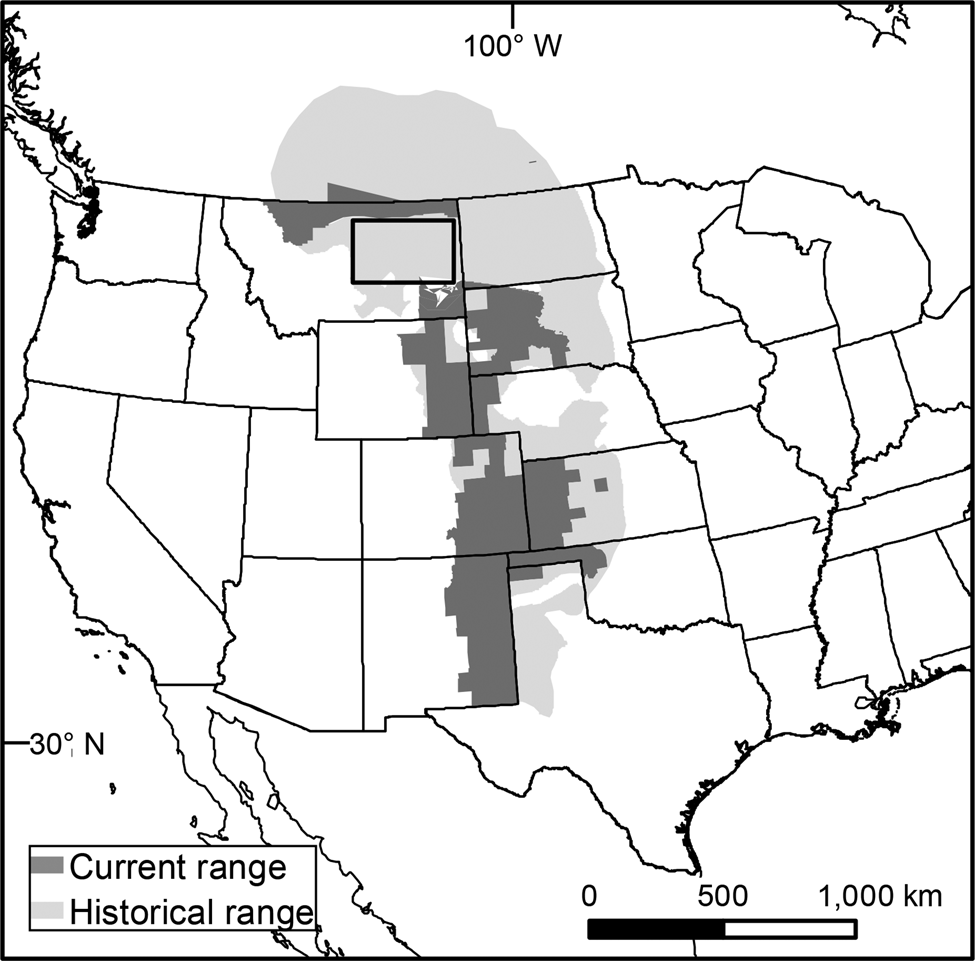
Fig. 1 Swift fox Vulpes velox historical and current range in the Great Plains of North America (adapted from Moehrenschlager & Sovada, 2016). The rectangle indicates the gap between the northern and southern swift fox populations.
In the mid 1980s swift foxes were successfully reintroduced to Alberta and Saskatchewan, Canada, through over a decade of translocation efforts (Smeeton & Weagle, Reference Smeeton and Weagle2000). This population has subsequently expanded into north-east Montana, with a resident population occurring north of the Milk River (Moehrenschlager & Sovada, Reference Moehrenschlager and Sovada2016; Fig. 1). Sightings of swift foxes south of the Milk River have been reported (Heather Harris, Montana Fish and Wildlife Parks, pers. comm., 2018), but no population has been established south of the river. Fort Belknap Indian Reservation lies south of the Milk River within the gap in the swift fox range (Fig. 2). The Reservation is home to the Assiniboine and Gros Ventre Tribes, who are coordinating a swift fox reintroduction to their sovereign lands.

Fig. 2 Landcover in the proposed reintroduction region between the Missouri and Milk Rivers.
The study area is within the Northern Great Plains of North America in a short grass and mixed grass prairie, with ephemeral streams. Landownership is a mixture of tribal trust, and private and public lands, with cattle ranching as the primary land use. There are two rivers running west to east through the study area, the Missouri River to the south and the Milk River to the north (Fig. 2). The proposed 15,230 km2 reintroduction area lies between these two rivers. The work presented here is part of the feasibility assessment conducted prior to the swift fox reintroduction.
Methods
Field surveys
We surveyed three components of swift fox diet (Table 1) using camera traps (Lagomorpha spp.), track plates (Rodentia spp.) and audio recordings (Orthoptera spp.). In addition, we surveyed coyotes via camera traps. We deployed camera traps (HyperFire 2, Reconyx, Holmen, USA) during July–October 2018 and May–September 2019, at 65 sites in 2018 (406 camera stations) and 142 sites in 2019 (852 camera stations), with 3–6 cameras set 250–400 m apart at each survey site for 3–6 weeks. Sites were resampled 2–3 times per year. In total, we collected data for 29,284 camera-trap nights (10,752 in 2018 and 18,532 in 2019). Cameras were set 50 cm above ground, facing north to avoid false triggers. Images were sorted, identified to species and stored in the eMammal repository (Shamon, Reference Shamon2021). We collected data at each camera location to assess detection bias: per cent vegetation cover (ground, grasses, forbs, shrubs and canopy), and mean shrub height within a 5-m radius circle in front of each camera, the distance at which the camera sensor was triggered in response to an approaching person, and whether or not the camera was set on an animal trail.
Table 1 Known swift fox Vulpes velox habitat requirements, with information sources.

We used track plates to estimate the probability of occurrence of rodent species (Zielinski, Reference Zielinski, Zielinski and Kucera1995; Wiewel et al., Reference Wiewel, Clark and Sovada2007; Hacker et al., Reference Hacker, Minter, Begon, Diggle, Serrano and Reis2016). We placed 299 track plates at 67 grassland sites, with 2–3 track plates set 250–400 m apart at each site for 1 week, and each site was sampled twice during May–September 2019. Plates were placed > 100 m from dirt roads, and baited with food (dry cat food and peanuts); 279 track plates were retrieved intact. Tracks were identified to species using field guides (Eder, Reference Eder2001; Elbroch, Reference Elbroch2003; Moskowitz, Reference Moskowitz2010) and validated by a professional track expert (Asaf Ben-David, Tel Aviv University, Tel Aviv, Israel).
We estimated Orthoptera diversity from audio recordings made with AudioMoths, a device that records frequencies up to 384 kHz (Hill et al., Reference Hill, Prince, Piña Covarrubias, Doncaster, Snaddon and Rogers2018). We first determined which hours to include in the analysis by evaluating recordings collected 24 h/day. We concluded that Orthoptera sounds were most common 3–5 hours after sunrise. This is a time of day when bird species are relatively quiet, enabling us to capture mostly insect sounds (Hutchinson, Reference Hutchinson2002; Brown & Handford, Reference Brown and Handford2003). We collected three consecutive 10-minute recordings during each sample day, and extracted the first minute of each recording for analysis. We recorded a total of > 1,500 hours at 222 locations across the study area (14–15 days per site), from which we analysed 157 hours (9,440 1-minute recordings).
Statistical analysis
We estimated occupancy for coyote and Leporidae spp. using presence/absence data from spatially and temporally repeated measures (camera-trap images), accounting for type II error (MacKenzie et al., Reference MacKenzie, Nichols and Lachman2002), with the occu function from the unmarked package (Fiske & Chandler, Reference Fiske and Chandler2011) in R 3.5.1 (R Core Team, 2018). This hierarchical model comprises both detection and site level functions. We first fitted detection explanatory variables with competing models and selected the best fit detection covariates based on Akaike information criterion (AIC) scores (Burnham & Anderson, Reference Burnham and Anderson2002). We then constructed occupancy models with different combinations of site level covariates (Table 2, Supplementary Table 1). Competing models were ranked and selected based on their AIC scores. The top models were extrapolated to the study area and used as covariates in the habitat suitability model.
Table 2 Details of explanatory variables used for coyote, Orthoptera, rodent and swift fox models.
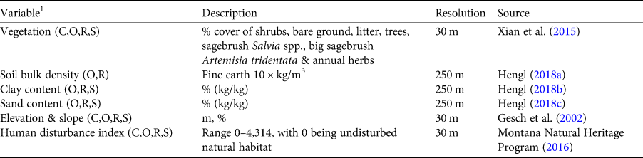
1C, coyote; O, Orthoptera; R, rodents; S, swift fox.
We modelled rodent species occurrence in response to habitat variables (Table 2), centring each response variable using the scale function in R (R Core Team, 2018). Rodent multivariate data (e.g. data of a number of species) were modelled in a generalized linear model framework with the binominal distribution using the function manyglm from the mvabund package in R (Wang et al., Reference Wang, Naumann, Eddelbuettel, Wilshire, Warton and Byrnes2019). We tested and evaluated the response of rodent occurrence to site level covariates using stepwise selection based on AIC scores. We used the function drop1() from the lme4 package in R (Fang et al., Reference Fang, Sun, Zhao, Lin, Sun and Gao2013; Bates et al., Reference Bates, Mächler, Bolker and Walker2015) to select variables for the final model. The top model was extrapolated over the study region for each rodent species.
We assessed Orthoptera diversity using the bioacoustic index (Boelman et al., Reference Boelman, Asner, Hart and Martin2007), which is the integral sum of the frequencies above the minimum volume of each sound curve (Villanueva-Rivera & Pijanowski, Reference Villanueva-Rivera and Pijanowski2018). We calculated the bioacoustic index for all 9,440 1-minute recordings using the bioacoustic_index function from the soundecology package in R (Boelman et al., Reference Boelman, Asner, Hart and Martin2007; Villanueva-Rivera & Pijanowski, Reference Villanueva-Rivera and Pijanowski2018). Orthoptera species diversity is affected by habitat heterogeneity (Evans, Reference Evans1988; Weiss et al., Reference Weiss, Zucchi and Hochkirch2013) and variation in nutrient availability (Bishop et al., Reference Bishop, O'Hara, Titus, Apple, Gill and Wynn2010), and insect stridulation (and thereby detectability) is influenced by meteorological variables (Riede, Reference Riede2017). Therefore, we modelled the values of the bioacoustic index in response to meteorological (Supplementary Table 2) and site level covariates (per cent grass and shrub cover, elevation, slope, and soil composition; Table 2). We extracted meteorological data from the ENV-DATA platform on Movebank (Kranstauber et al., Reference Kranstauber, Cameron, Weinzerl, Fountain, Tilak, Wikelski and Kays2011; Dodge et al., Reference Dodge, Bohrer, Weinzierl, Davidson, Kays and Douglas2013). We used linear regression to model the data and performed a stepwise model selection using the lm and stepAIC functions in the MASS package in R (Venables & Ripley, Reference Venables and Ripley2002; Ripley et al., Reference Ripley, Venables, Bates, Hornik, Gebhardt and Firth2019). The final model was extrapolated to the region by fixing all meteorological variables to optimal conditions (zero wind, precipitation and cloud cover, median temperature) and allowing site level covariates to vary.
Habitat suitability models
We developed and validated a swift fox habitat suitability model using four steps. Firstly, we reviewed variables important for swift fox ecology (Table 1). Secondly, we constructed a habitat suitability model for the swift fox based on remotely-sensed and publicly available geographical interpolated data (Tables 1 & 2). Variables known to have an inverse relationships with swift fox occurrence were rescaled using an exponential decaying function. Thirdly, we used field surveys to model the distribution of the main prey species of the swift fox, and the occupancy of coyotes (a swift fox predator). We extrapolated the models and created two spatial layers: (1) a threat layer (coyote occupancy), and (2) a resource layer comprising each diet variable (rodents, insects, rabbits) and scaled to 0–1. Additional weight was given to rabbit species and ground squirrels Urocitellus richardsonii compared to small rodent species and insects (4:1 respectively) based on known swift fox diet (Table 1). Fourthly, we evaluated the contribution of each of the predictors created in the second and third steps in estimating swift fox habitat suitability. Because of the proximity of an existing swift fox population to the north, it was possible to assess the importance of each of the covariates in relation to known swift fox locations. The model covariates created in step two and three were extrapolated north of the Milk River where the northern swift fox population occurs (Fig. 1).
We obtained 418 known swift fox locations collected during 1997–2017 (Montana Natural Heritage Program, 2019). Known locations were modelled in response to the three covariates using the rspf function from the ResourceSelection package in R (Lele, Reference Lele2009). Swift fox locations are presence-only data, and therefore we extracted 10 random points within a 20 km2 buffer around each known location as background points (4,180 points in total). The buffer distance was selected based on known swift fox home range estimates in a similar climate (Olson & Lindzey, Reference Olson and Lindzey2002). We ran 1,000 iterations of each candidate model. We used multi-model inference to select competing models based on their AIC scores. We used the Hosmer and Lemeshow test to assess model goodness of fit (Hosmer & Lemeshow, Reference Hosmer and Lemeshow2000). We then assessed the overlap between the top habitat suitability model based on known swift fox locations and two data layers; remote data and all three covariates combined. The latter is a summation of remote data, resources, and threat layers scaled to 0–1. The upper quartile of the swift fox habitat suitability model included values > 0.56. We used these values as the cutoff to calculate the overlap between data layers.
Results
Field surveys
In total we detected coyotes and Leporidae on 521 and 235 occasions, respectively. Coyotes were detected in areas with lower shrub cover and shrub height, and steeper slope (Table 3). Leporidae were detected in areas with lower slope, and higher canopy and shrub cover (Table 3). We identified seven rodent species via tracks on 279 track plates. We modelled the probability of occurrence of the three most prevalent species (Urocitellus richardsonii, Reithrodontomys megalotis, Peromyscus maniculatus), which were detected on 8, 67, and 63 track plates respectively. All candidate rodent models were similar and included % sand, % clay, human disturbance index, and soil bulk density (Table 4). Bioacoustic index values were modelled in response to landscape and methodological variables. The top model included four detection covariates (all meteorological) and three site level covariates (% clay, herbaceous cover and slope; Table 5). The bioacoustics index was positively affected by clay soil content, and negatively affected by % herbaceous cover (Table 5).
Table 3 Occupancy models (ψ) for the coyote and Leporidae spp., selected based on AIC rank. Occupancy estimation based on camera-trap data collected during June–October 2018 and May–September 2019 in the Northern Great Plains, Montana, USA (Fig. 1).

Table 4 Estimated occurrence of rodents using a multivariate generalized linear framework, with top model selected using a stepwise process based on AIC scores. Data were collected via track plates during May–September 2019.

Table 5 Bioacoustic index values in response to methodological and site level covariates, with top model selected using a stepwise selection process. Data were collected via audio recordings at grassland sites during May–September 2019.

Habitat suitability models
The top habitat suitability model included all three covariates based on field surveys and the remote data (Table 6). The resources and remote data covariates were positive predictors of swift fox occurrence, and coyote occupancy was a negative predictor of swift fox occurrence (Table 7, Supplementary Table 1). Overlap between the remote data model (Fig. 3a) and the top swift fox habitat suitability model (Fig. 3d) was 38% (Fig. 4a), and overlap between the field covariate model and swift fox habitat suitability model was 89% (Fig. 4b). The remote data model and top habitat suitability model produced estimates of 4,579 and 5,456 km2 of suitable area, respectively (with suitability considered as values > 0.56). The habitat suitability model containing both field covariates and remote sensing data had a 16% higher estimated highly suitable area compared to the remote sensing model.

Fig. 3 Swift fox habitat suitability covariates and leading model: (a) habitat suitability based on remote sensing data only, (b) swift fox resources layer, (c) coyote occupancy, (d) swift fox leading habitat suitability model using resource selection function, and (e) the same area, showing the swift fox range, major rivers and Fort Belknap Indian Reservation.
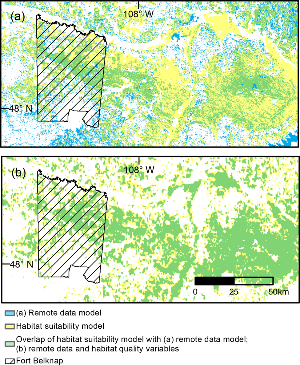
Fig. 4 (a) Overlap between habitat suitability model (~remote data + resources + coyote) and remote data model, and (b) overlap between habitat suitability model (~remote data + resources + coyote) and remote data and habitat quality variables model. Values > 0.56 (upper quartile of the habitat suitability model) were considered in overlap calculations.
Table 6 Swift fox habitat suitability models ranked by AIC. Known swift fox locations were modelled in response to a habitat suitability model based on remote data (remote sensing and geographically interpolated data, RD), swift fox diet resources (Resources), and coyote occupancy.

1Hosmer and Lemeshow goodness of fit.
Table 7 Swift fox habitat suitability model, with top model selected by a backward stepwise process. Known swift fox locations were modelled in response to three layer products: habitat suitability model based on remotely-sensed data and geographically interpolated data (RD), swift fox diet resources layer, and coyote occupancy layer.

Discussion
We found that habitat quality variables derived from field surveys improved habitat suitability model predictions for the swift fox. We identified significant differences in estimates of suitable habitat between a model based on remote data and a model that also included habitat quality variables based on field surveys. The differences in the amount of potentially suitable habitat and its distribution highlight how habitat quality variables can greatly impact model predictions, and the limitation of relying solely on remote data. In this case, improved model estimates suggest the reintroduction area can support more individuals, which increases the probability of success (Lewis et al., Reference Lewis, Powell and Zielinski2012).
Habitat suitability variables are not necessarily a proxy for habitat quality. Habitat suitability models are defined as the empirical correlation between species occurrence and environmental conditions (Bradley et al., Reference Bradley, Olsson, Wang, Dickson, Pelech, Sesnie and Zachmann2012), and those variables that impact species fitness and demographics are indicative of habitat quality (Johnson, Reference Johnson2005). Habitat quality can be measured two ways: (1) by the variation in individual or population demographics, or (2) by the variation in environmental conditions that affect habitat selection and fitness (Johnson, Reference Johnson2005). Larson et al. (Reference Larson, Thompson, Millspaugh, Dijak and Shifley2004) suggested including habitat quality variables that impact demographics (via population viability analysis) in habitat suitability models. In the case of reintroductions when there is no established population, modelling habitat suitability is only possible through a series of underlying assumptions and model simulations. A third way is to include environment variables indicative of habitat quality (e.g. available resources or predation risk) in habitat suitability models. In reintroductions, the quality of release sites should be assessed beforehand (Cheyne, Reference Cheyne2006), but assessment at a local scale may be misleading and may not reflect the quality of the entire landscape. In the case of the swift fox, our approach entails extensive field surveys and additional modelling, to create covariates that represent habitat quality at the landscape level.
Some remote data products are indicative of habitat quality and can be used in specific cases to inform reintroductions. Such products have been shown to increase model accuracy, and combined with their free accessibility they are appealing for such analysis (Bradley et al., Reference Bradley, Olsson, Wang, Dickson, Pelech, Sesnie and Zachmann2012). For example, the normalized difference vegetation index is commonly used as a proxy of forage quality for ungulates, or as proxy for insect biomass (Pettorelli et al., Reference Pettorelli, Ryan, Mueller, Bunnefeld, Jedrzejewska, Lima and Kausrud2011; Fernández-Tizón et al., Reference Fernández-Tizón, Emmenegger, Perner and Hahn2020). However, caution should be used when interpreting models based on remote data products, especially for predators that rely on prey densities. For example, throughout their range, swift foxes were eliminated from seemingly suitable habitat as a result of prey depletion and predator persecution (Zimmerman, Reference Zimmerman1998). In their case the quality of the habitat was compromised even though the vegetation remained intact. Predictive models based on remote data products suggest that there is ample swift fox suitable habitat throughout the species’ historic range that is yet to be recolonized (Sovada et al., Reference Sovada, Woodward and Igl2009). Sovada et al. (Reference Sovada, Woodward and Igl2009) suggested that swift foxes are not recolonizing these areas for two main reasons: (1) dispersing swift foxes have high mortality rates, and (2) interspecific competition with other meso-canids is hindering recolonizations. Our findings support their hypotheses, and we add that other factors influencing habitat quality, such as resource availability, should be considered. Other studies have found that low prey densities influenced reintroduction success of mesocarnivores (Moehrenschlager et al., Reference Moehrenschlager, Cypher, Ralls, List, Sovada, MacDonald and Sillero-Zubiri2004; Jachowski et al., Reference Jachowski, Gitzen, Grenier, Holmes and Millspaugh2011; Scrivner et al., Reference Scrivner, O'Farrell, Hammer and Cypher2016; Parsons et al., Reference Parsons, Lewis, Gardner, Chestnut, Ransom, Werntz and Prugh2019).
Interspecific competition, as hypothesized by Sovada et al. (Reference Sovada, Woodward and Igl2009), cannot be assessed from remote data products. Predator composition has changed throughout the swift fox's historical range. The coyote is now the largest canid and most abundant mesocarnivore in the Great Plains grasslands (Miller & Harlow, Reference Miller and Harlow2012). Coyotes limit both swift fox and kit fox populations (White & Garrott, Reference White and Garrott1997; Kamler et al., Reference Kamler, Ballard, Gilliland, Lemons and Mote2003), and reintroductions of both species were hindered by competition with coyotes (Moehrenschlager et al., Reference Moehrenschlager, Cypher, Ralls, List, Sovada, MacDonald and Sillero-Zubiri2004). Kit fox populations increase with high prey densities and decrease with high coyote density (Standley et al., Reference Standley, Berry, O'Farrell and Kato1992; Arjo et al., Reference Arjo, Gese, Bennett and Kozlowski2007). However, White & Garrott (Reference White and Garrott1997) found that predation by coyotes limits kit fox numbers in conjunction with low prey abundance, possibly because increased prey density allowed kit foxes greater dietary breadth and use of dens throughout the year, facilitating coexistence with coyotes (Cypher & Spencer, Reference Cypher and Spencer1998). Kamler et al. (Reference Kamler, Ballard, Gilliland, Lemons and Mote2003) found that swift fox population source and sink properties are directly tied to coyote densities and suggested that coyote control can shift swift fox populations from sink to source.
In previous swift fox reintroductions, coyotes were culled to ensure that the fox population was not predated (Honness et al., Reference Honness, Phillips and Kunkel2008). However, culling coyotes has only short-term effects on their density, and when coyotes were culled in an area with an established swift fox population it did not affect fox density (KARKI et al., Reference Karki, Gese and Klavetter2007). In other parts of the world, culling was found to be an ineffective method of control for generalist canids that fill a niche similar to coyotes (Baker & Harris, Reference Baker and Harris2006; Kapota & Saltz, Reference Kapota and Saltz2018). The potential negative impact of interspecific competition between swift fox and coyote on reintroduction success warrants assessment of these risks at release sites, and supports the inclusion of variables that affect survival and fitness in habitat suitability assessments.
We did not include people as a potential threat in our analysis because there is no perceived social opposition or risks associated with social tolerance of the swift fox. However, social tolerance can affect fitness of species (Sage, Reference Sage2019) and ultimately the success of reintroductions. When applicable, we suggest including landscape level assessments of social tolerance, and other gradients of anthropogenic impacts in habitat suitability models used for reintroduction.
In summary, based on our findings and other research, we conclude that including ground-based assessments of habitat quality improves predictions of habitat suitability for reintroductions. The addition of habitat quality data in our case study increased the area predicted to be suitable, and thus the estimated carrying capacity of the landscape. These model outcomes influenced the planning of a swift fox reintroduction led by the Assiniboine and Gros Ventre Tribes of Fort Belknap Indian Reservation.
Acknowledgements
We thank the Fort Belknap Indian Community, C.M. Russell Wildlife Refuge, Bureau of Land Management, and the American Prairie Reserve for access to lands; the American Prairie Reserve for providing the space to conduct our research; Justin Kitzes, University of Pittsburgh, for supplying audio recorders; and Asaf Ben-David, Tel Aviv University, for validating track identifications.
Author contributions
Study design, fieldwork: all authors; data analysis: HS, ZP; writing: all authors.
Conflicts of interest
None.
Ethical standards
This research abided by the Oryx guidelines on ethical standards.


 Open access