


1. Introduction
Thermal convection impacts natural processes in the atmosphere and oceans. It also finds industrial applications in solar panels, electronics cooling and chemical vapour deposition to name a few. When forced and natural convection act simultaneously, a regime of mixed convection occurs and the mechanisms of inertia, shear and buoyancy compete. For example, a typical chemical vapour deposition reactor can be modelled by a mixed convection boundary layer where a shear flow develops over a surface heated from below. To ensure that the film is uniform throughout the reactor, it is necessary to delay flow transition so that purity, thickness and adhesion of the deposited films are controlled (Jensen, Einset & Fotiadis Reference Jensen, Einset and Fotiadis1991; Mahajan Reference Mahajan1996).
Flows involving mixed convection have been investigated both numerically as well as experimentally (Wu & Moin Reference Wu and Moin2010; Dennis & Siddiqui Reference Dennis and Siddiqui2021a,Reference Dennis and Siddiquib, Reference Dennis and Siddiqui2022). However, most studies analyse turbulence properties, while fewer address stability and transition effects. The majority of the flow stability studies involving mixed convection were performed for Poiseuille–Rayleigh–Bénard (PRB) flows. Nicolas, Luijkx & Platten (Reference Nicolas, Luijkx and Platten2000) investigated the influence of temperature gradients in PRB flows using bi-global modal stability analysis. They found that the critical Rayleigh number for the onset of longitudinal rolls decreases as the aspect ratio of the channel is increased.
Sameen & Govindarajan (Reference Sameen and Govindarajan2007) employed a transient growth analysis of PRB flow using a temperature-dependent viscosity formulation and John Soundar Jerome, Chomaz & Huerre (Reference John Soundar Jerome, Chomaz and Huerre2012) presented a similar study for a buoyancy-driven formulation using the Oberbeck–Boussinesq (OB) approximation. Sameen & Govindarajan (Reference Sameen and Govindarajan2007) found that a smaller viscosity near the wall has a larger stabilizing effect for water. They also found that the Prandtl number has an important impact on transient growth, but not on the time-asymptotic decay. On the other hand, viscosity stratification was found to have an important impact on exponential growth, but not on algebraic growth. John Soundar Jerome et al. (Reference John Soundar Jerome, Chomaz and Huerre2012) observed that PRB flow has a more energetic transient growth when compared with the plane Poiseuille case. Such transient growth was also found to occur for a longer period due to thermal effects. More recently, Vo, Potherat & Sheard (Reference Vo, Potherat and Sheard2017) investigated the linear and modal stability of PRB flows of liquid metals subjected to transverse magnetic fields due to their use in fusion reactors. Those authors considered the OB approximation, deriving a reduced set of disturbance equations composed of the energy equation coupled with the Orr–Sommerfeld equation modified to account for thermal and magnetic effects. By doing so, they were able to investigate instabilities arising from the interactions among shear, thermal stratification and magnetic damping effects.
Differently from PRB flow, a mixed convection boundary layer does not occur in a confined domain. Therefore, the base flow has velocity and thermal gradients near the wall, while the far-field profiles are uniform. Early investigations focused on how the base flow obtained from steady boundary layer equations was influenced by the surface temperature and the distance from the plate leading edge in forced, free and mixed convection (Sparrow, Eichhorn & Gregg Reference Sparrow, Eichhorn and Gregg1959; Sparrow, Quack & Boerner Reference Sparrow, Quack and Boerner1970; Sparrow & Yu Reference Sparrow and Yu1971; Chen, Sparrow & Mucoglu Reference Chen, Sparrow and Mucoglu1977; Schneider Reference Schneider1979). Those studies showed that base flow variations are only significant at extreme thermal conditions, i.e. high Richardson numbers. Wu & Cheng (Reference Wu and Cheng1976) and Cheng & Wu (Reference Cheng and Wu1976) were among the first to perform a linear, local and modal stability analysis of this problem. Their analyses of an OB approximated base flow over a horizontal plate provided critical Grashof and Reynolds numbers, showing that increasing the Prandtl number has a destabilizing effect. Those studies were extended by Chen & Mucoglu (Reference Chen and Mucoglu1979), who considered non-parallel base flow effects when performing their stability analysis to investigate the impact of these effects on the neutral curves for different Prandtl and Richardson numbers. It was found that, for moderate values of the Richardson number, the non-parallel and parallel approximations provided almost identical results.
Research on this topic remained dormant for three decades until it was picked up again in the context of atmospheric sciences. Such boundary layers are supposed to be stable to inviscid disturbances (Chimonas Reference Chimonas2002), but compressibility and non-OB effects can change this when the surface is inclined (Candelier, Le Dizès & Millet Reference Candelier, Le Dizès and Millet2012). Viscous instabilities were first investigated using the Navier–Stokes equations by Wu & Zhang (Reference Wu and Zhang2008) for horizontal plates. They performed a linear, local and modal stability analysis based on triple-deck theory for large Reynolds numbers. In such supercritical parametric conditions, stratification has a stabilizing effect on the spatial growth rates. However, stabilization is not uniform across all modes, shifting the dominant unstable modes towards higher frequencies. It is also worth pointing out that the linear, local and modal stability of a horizontal flow over a vertical plate has been considered as well (Chen, Bai & Le Dizès Reference Chen, Bai and Le Dizès2016). However, a couple of issues are worth noting. The first one is base flow accuracy (Teixeira & Alves Reference Teixeira and Alves2017), since an ad hoc hyperbolic function was used instead of a similarity solution. The second one is the unstable nature of the flow (Huerre & Monkewitz Reference Huerre and Monkewitz1990), since a temporal instead of spatial stability analysis was performed under supercritical parametric conditions. Finally, both modal and non-modal (Schmid Reference Schmid2007) linear stability analyses of mixed convection boundary layers appeared recently when Parente et al. (Reference Parente, Robinet, De Palma and Cherubini2020) studied a stably stratified horizontal boundary layer. The modal analysis was performed under the scope of spatial stability and the non-modal analysis was evaluated using a direct-adjoint looping procedure. It was found that the Richardson number has an impact on the optimal gain and the optimal streamwise wavenumber, which considerably departs from zero. They also showed that the latter was due to the competition between two distinct effects, the lift-up and the Orr mechanisms.
Although modal (Reed, Saric & Arnal Reference Reed, Saric and Arnal1996) and non-modal (Andersson, Berggreen & Henningson Reference Andersson, Berggreen and Henningson1999; Corbett & Bottaro Reference Corbett and Bottaro2000; Monokrousos et al. Reference Monokrousos, Åkervik, Brandt and Henningson2010) linear stability theories have been extensively applied to Blasius boundary layers, the aforementioned examples illustrate that the same is not true for their mixed convection counterparts. In fact, the study by Parente et al. (Reference Parente, Robinet, De Palma and Cherubini2020) is the first to do so in regards to the latter theory. The present study extends their linear and local analysis in two meaningful ways, namely it (i) applies modal as well as non-modal theory, where the latter is done through an analysis of the pseudospectra (Trefethen & Embree Reference Trefethen and Embree2005), to unstably stratified horizontal boundary layers and (ii) uses input–output analysis (Jovanović Reference Jovanović2021) to study the optimal flow response with respect to imposed disturbances, which could in turn provide insights in terms of control strategies for the present flows.
2. Governing equations of the linearized model
The small-amplitude-disturbance governing equations for mixed convection Blasius boundary layer flow are obtained by linearizing the OB approximated Navier–Stokes equations (Chandrasekhar Reference Chandrasekhar1961). These equations are linearized with respect to a base flow obtained by solving the Blasius self-similar solution for both the velocity and thermal boundary layers. The linearization is followed by non-dimensionalization using the free-stream velocity  $U_{\infty }^*$, the displacement thickness $\delta ^*$ and the temperature difference $\Delta T^* = T_s^*-T_\infty ^*$, where the superscript $^*$ stands for dimensional variables. Here, $T_s^*$ and $T_\infty ^*$ are the temperature at the surface and the far field, respectively. A schematic containing the self-similar solutions, the adopted coordinate system and the parameters used for the non-dimensionalization of the system of equations is shown in figure 1.

Figure 1. A schematic of the flows under investigation. It contains the coordinate system  $(x,y,z)$ $=$ (streamwise, spanwise, wall-normal), the variables used to non-dimensionalize the equations ( $U_{\infty }^*, \delta ^*, T_s^*, T_\infty ^*$) and a representation of the Blasius self-similar solution for both the velocity $(U(z))$ and thermal ( $\varTheta (z)$) laminar boundary layers.
The linearized form of the governing equations is written in non-dimensional form as
 \begin{equation} \left.\begin{gathered} \dfrac{\partial u_i}{\partial x_i} = 0{ ,} \\ \dfrac{\partial u_i}{\partial t} +U\dfrac{\partial u_i}{\partial x} +u_j\dfrac{\partial U}{\partial x_j}\delta_{i1} ={-}\dfrac{\partial p}{\partial x_i} +Ri_{\delta^*}\,\theta\delta_{i3} +\dfrac{1}{Re_{\delta^*}}\dfrac{\partial^2u_i}{\partial x_j \partial x_j}\quad \text{and}\\ \dfrac{\partial \theta}{\partial t} +U\dfrac{\partial \theta}{\partial x} + u_i\dfrac{\partial \varTheta}{\partial x_i} = \dfrac{1}{ Re_{\delta^*}Pr}\dfrac{\partial^2\theta}{\partial x_i \partial x_i} , \end{gathered}\right\} \end{equation}
where  $x_i=(x_1,x_2,x_3)=(x,y,z)$ and $u_i=(u_1,u_2,u_3)=(u,v,w)$ represent the spatial coordinates and velocity disturbances in the streamwise, spanwise and wall-normal directions, respectively. The time is represented by $t$, the pressure disturbance by $p$, the Kronecker delta by $\delta _{ij}$ and the temperature disturbance by $\theta$. The steady laminar profiles for the streamwise velocity and temperature are given by $U$ and $\varTheta$, respectively. Both vary only along the wall-normal direction.
The dimensionless parameters arising in the equations are the Richardson number  $Ri_{\delta ^*} = Ra_{\delta ^*}/(Re_{\delta ^*}^2Pr)$, Reynolds number $Re_{\delta ^*} = U^*_{\infty }\delta ^*/\nu ^*$, Prandtl number $Pr = \nu ^*/\alpha ^*$ and Rayleigh number $Ra_{\delta ^*} = g^*\beta ^*\Delta T^*\delta ^{*3}/\nu ^*\alpha ^*$, where $\rho ^*$ is the density, $g^*$ is the gravitational acceleration, $\beta ^*$ is the volumetric thermal expansion coefficient, $\alpha ^*$ is the thermal diffusivity and $\nu ^*$ is the kinematic viscosity. The present non-dimensional parameters characterize the ratios of buoyancy to flow shear ( $Ri$), inertial to viscous forces ( $Re$), momentum to thermal boundary layer thicknesses ( $Pr$) and buoyancy to viscous and thermal diffusion ( $Ra$).
The flow disturbances are assumed to be periodic in the streamwise ( $x$) and spanwise ( $y$) directions, allowing the application of a Fourier transform in both cases as
 \begin{equation} \boldsymbol{q}(x,y,z,t) = \boldsymbol{\hat{q}}(z,t)\exp{\{\text{i}(k_{\delta^*}x+m_{\delta^*}y)\}}, \quad\text{where}\ \boldsymbol{q}=(u,v,w,\theta,p)^{\rm T} , \end{equation}
the eigenvalues  $k_{\delta ^*}$ and $m_{\delta ^*}$ represent the streamwise and spanwise wavenumbers, respectively, $\boldsymbol {\hat {q}}$ represents their respective eigenfunctions and i stands for the imaginary number. By applying (2.2) to the governing equations defined in (2.1) and discretizing the system in the wall-normal direction ( $z$), the following system is obtained:
 \begin{equation} \left.\begin{gathered} 0 = \text{i}k_{\delta^*}\hat{u}+\text{i}m_{\delta^*}\hat{v}+D\hat{w} { ,} \\ \dfrac{\partial \hat{u}}{\partial t} + U\text{i}k_{\delta^*}\hat{u}+\hat{w}DU ={-}\text{i}k_{\delta^*}\hat{p} +\dfrac{1}{Re_{\delta^*}}[-\hat{u}(k_{\delta^*}^2+m_{\delta^*}^2)+D^2\hat{u}]{,}\\ \dfrac{\partial \hat{v}}{\partial t} + U\text{i}k_{\delta^*}\hat{v} ={-}\text{i}m_{\delta^*}\hat{p} +\dfrac{1}{Re_{\delta^*}}[-\hat{v}(k_{\delta^*}^2+m_{\delta^*}^2)+D^2\hat{v}]{,}\\ \dfrac{\partial \hat{w}}{\partial t} +U\text{i}k_{\delta^*}\hat{w} ={-}D\hat{p} +Ri_{\delta^*}\hat{\theta}+\dfrac{1}{Re_{\delta^*}}[-\hat{w}(k_{\delta^*}^2+ m_{\delta^*}^2)+D^2\hat{w}]\quad \mbox{and}\\ \dfrac{\partial \hat{\theta}}{\partial t} + U\text{i}k_{\delta^*}\hat{\theta}+ \hat{w}D\varTheta = \dfrac{1}{Re_{\delta^*}Pr}[-\hat{\theta}(k_{\delta^*}^2+m_{\delta^*}^2)+D^2\hat{\theta}]{,} \end{gathered}\right\} \end{equation}
where the wall-normal derivatives  $D=\partial /\partial z$ are discretized using a sixth-order finite difference scheme. Dirichlet boundary conditions are imposed for all variables $(\hat {\boldsymbol {q}}=0)$ at the wall, except for the pressure, which is obtained by evaluating the wall-normal momentum equation from (2.3). Noting that both temperature and velocity disturbances are null at the wall leads to $D \hat {p} = (1/Re_{\delta ^*}) D^2\hat {w}$ at $z=0$. Dirichlet boundary conditions are also applied for all variables $(\hat {\boldsymbol {q}}=0)$ in the far field (Parente et al. Reference Parente, Robinet, De Palma and Cherubini2020; Schmid & Henningson Reference Schmid and Henningson2000) except for pressure, since the mass conservation equation is solved directly. The robustness of these choices was evaluated by verifying the sensitivity of the results to other boundary conditions, as discussed in further detail in Appendix A.
3. Linear stability and resolvent analyses
The set of equations in (2.3) can be rewritten in vector form as
 \begin{equation} \boldsymbol{\mathsf{R}}\dfrac{\partial}{\partial t}\hat{\boldsymbol{q}} = \boldsymbol{\mathsf{L}}\hat{\boldsymbol{q}} {,} \end{equation}
where  $\boldsymbol{\mathsf{R}}$ is a singular matrix. The solution of (3.1) is obtained by a generalized eigenvalue problem for $\boldsymbol{\mathsf{R}}$ and $\boldsymbol{\mathsf{L}}$. As shown by Peters & Wilkinson (Reference Peters and Wilkinson1970), the solution of the generalized eigenvalue problem is equivalent to the solution of a conventional eigenvalue problem. The linear system associated with the latter can be written as
 \begin{equation} \dfrac{\partial}{\partial t}\hat{\boldsymbol{q}} = \tilde{\boldsymbol{\mathsf{L}}}\hat{q} { ,} \end{equation}
where  $\tilde {\boldsymbol{\mathsf{L}}}= \boldsymbol{\mathsf{D}}^{\boldsymbol{-1}} \boldsymbol{\mathsf{L}} (\boldsymbol{\mathsf{D}}^{\boldsymbol{H}})^{\boldsymbol{-1}}$, $\boldsymbol{\mathsf{D}}$ is obtained by the Cholesky decomposition $\boldsymbol{\mathsf{R}} = \boldsymbol{\mathsf{DD}}^{\boldsymbol{H}}$, since $\boldsymbol{\mathsf{R}}$ is singular, and the superscript $H$ refers to the Hermitian. The solution of (3.2) leads to eigenvalue and eigenvector matrices $\boldsymbol {\varLambda }$ and $\boldsymbol{\mathsf{V}}$, respectively, which are identical to those from (3.1). For the modal analysis, a Laplace transform can be applied to model the temporal dynamics since the time-asymptotic stability of a steady state is considered. This allows the eigenfunctions to be rewritten as
 \begin{equation} \hat{\boldsymbol{q}}(z,t) = \tilde{\boldsymbol{q}}(z)\exp{(-\text{i}\omega t)} { ,} \end{equation}
which can be substituted into (3.2) to yield the eigenvalue problem,
 \begin{equation} -\text{i}\omega\tilde{\boldsymbol{q}} = \tilde{\boldsymbol{\mathsf{L}}}\tilde{\boldsymbol{q}} { ,} \end{equation}
for imposed real values of the wavenumbers ( $k_{\delta ^*}$, $m_{\delta ^*}$). Solving (3.4) yields the complex eigenspectrum $\omega$. In the present problem, shear effects are represented by the term $\hat {w}DU$ in (2.1). They can lead to a loss of orthogonality between eigenvectors of the linear dynamical system. When strong enough, this allows for a temporary energy growth at finite times even when this system displays a time-asymptotic ( $t\rightarrow \infty$) energy decay (Schmid Reference Schmid2007). In order to investigate such non-modal effects, a resolvent analysis is employed to uncover the flow response with respect to imposed disturbances, an approach popularized by McKeon & Sharma (Reference McKeon and Sharma2010) and widely used today (Ricciardi, Wolf & Taira Reference Ricciardi, Wolf and Taira2022).
In order to perform a componentwise input–output analysis, the linear system defined in the modal approach, i.e. (3.2), is rewritten to include a spatially distributed body force  $\boldsymbol {f}$. It can have different interpretations, such as nonlinear effects retained in the formulation (McKeon & Sharma Reference McKeon and Sharma2010) or an external input or excitation of the flow field (Jovanović & Bamieh Reference Jovanović and Bamieh2005). Following a state-space representation, a supplementary equation is introduced to evaluate a user-specified output component $\boldsymbol {g}$ of the full state vector $\hat {\boldsymbol {q}}$ as
 \begin{equation} \dfrac{\partial}{\partial t}\hat{\boldsymbol{q}} = \tilde{\boldsymbol{\mathsf{L}}}\hat{\boldsymbol{q}}+ \boldsymbol{\mathsf{B}}\boldsymbol{f} \quad \text{and} \quad \boldsymbol{g} = \boldsymbol{\mathsf{C}}\hat{\boldsymbol{q}} { ,} \end{equation}
where  $\boldsymbol{\mathsf{B}}$ and $\boldsymbol{\mathsf{C}}$ determine how the forcing enters the dynamics and which responses are analysed, respectively. Assuming a harmonic forcing, the system response becomes
 \begin{equation} \hat{\boldsymbol{g}} = \boldsymbol{\mathsf{C}}(\text{i}\omega \boldsymbol{\mathsf{I}}-\tilde{\boldsymbol{\mathsf{L}}})^{{-}1}\boldsymbol{\mathsf{B}}\hat{\boldsymbol{f}} { ,} \end{equation}
where  $(\boldsymbol {f},\boldsymbol {g}) = (\hat {\boldsymbol {f}},\hat {\boldsymbol {g}}) \exp (\textrm {i}\omega t)$ and $\boldsymbol{\mathsf{I}}$ is the identity matrix.
The maximum energy gain of the system due to forcing is then defined as the ratio between output and input maximized over all possible forcing profiles  $\hat {\boldsymbol {f}}$ for a given frequency $\omega$. Doing so leads to the input–output norm $R(\omega )$, which returns the resolvent norm when the forcing and response matrices are given by $\boldsymbol{\mathsf{B}} = \boldsymbol{\mathsf{C}} = \boldsymbol{\mathsf{I}}$. It can be represented as
 \begin{equation} R(\omega) = \max_{\hat{\boldsymbol{f}}}\dfrac{||\hat{\boldsymbol{g}}||^2_E}{||\hat{\boldsymbol{f}}||^2_E} =||\boldsymbol{\mathsf{C}}({\rm i}\omega\boldsymbol{\mathsf{I}}-\tilde{\boldsymbol{\mathsf{L}}})^{{-}1}\boldsymbol{\mathsf{B}}||^2_E = ||\boldsymbol{\mathsf{C}}({\rm i}\omega\boldsymbol{\mathsf{I}}-\tilde{\boldsymbol{\mathsf{L}}}_E)^{{-}1}\boldsymbol{\mathsf{B}}||^2_2 { .} \end{equation}
It is important to note that the term  $E$ refers to an energy norm that takes into account kinetic and thermal energies. The latter can be interpreted as the disturbance thermal potential energy (John Soundar Jerome et al. Reference John Soundar Jerome, Chomaz and Huerre2012). The energy norm can be written as
 \begin{equation} E(t) = \int_{0}^{\infty}\tfrac{1}{2}\left[|\hat{u}|^2+|\hat{v}|^2+|\hat{w}|^2+Ri_{\delta^*}|\hat{\theta}|^2\right]{\rm d}z { .} \end{equation}
As discussed by the previous authors, the form of a thermal energy norm is arbitrary. Here, following a reasoning similar to that provided in the previous reference, the thermal energy norm for the mixed convection boundary layer problem is weighted by  $Ri_{\delta ^*}$, which returns the classical kinetic energy norm when $Ri_{\delta ^*}=0$. The energy norm can be applied directly into $\tilde {\boldsymbol{\mathsf{L}}}$ by the following transformation:
 \begin{equation} \tilde{\boldsymbol{\mathsf{L}}}_E = (\boldsymbol{\mathsf{HEV}})\boldsymbol{\varLambda}(\boldsymbol{\mathsf{HEV}})^{{-}1} { ,} \end{equation}
where  $\boldsymbol{\mathsf{E}} = \textrm {diag}(\boldsymbol{\mathsf{I}},\boldsymbol{\mathsf{I}},\boldsymbol{\mathsf{I}},\sqrt {Ri_{\delta ^*}},0) / \sqrt {2}$ and $\boldsymbol{\mathsf{H}}$ accounts for the integration weights due to grid stretching in the domain discretization.
The pseudospectrum and the componentwise input–output analyses are performed by applying singular value decomposition to the resolvent and input–output operators, respectively (Jovanović & Bamieh Reference Jovanović and Bamieh2005). The optimal forcing and its respective response are given by the left and right singular vectors of the dominant singular value, respectively (Schmid & Brandt Reference Schmid and Brandt2014). It is important to mention that the numerical tool has been validated through a comparison of results for the Blasius boundary layer obtained by Schmid & Henningson (Reference Schmid and Henningson2000) in terms of the eigenspectrum and eigenvectors, and also with Monokrousos et al. (Reference Monokrousos, Åkervik, Brandt and Henningson2010) and Nogueira et al. (Reference Nogueira, Cavalieri, Hanifi and Henningson2020) for the resolvent analysis. The wall-normal domain size selected for the present investigation is  $z_{max} = 30\delta$, with $\delta$ standing for the boundary layer thickness. A result sensitivity analysis with respect to domain size is provided in Appendix B.
4. Results
In this section, we assess the effects of inertia, shear and buoyancy on the linear and local instabilities in a mixed convection boundary layer over horizontal plates. First, a temporal and modal stability analysis is applied to identify the onset of instability for different values of the Reynolds, Prandtl and Richardson numbers. Then, a resolvent analysis is applied to investigate the effects of non-normality near the marginal stability parametric conditions. Finally, this latter analysis is employed once again, but now in terms of a componentwise input–output approach, to investigate the receptivity to external disturbances.
4.1. Neutral curves, eigenspectra and pseudospectra
Figure 2 presents the neutral curves for the Prandtl numbers  $Pr = 0.7$ and $7.0$, which are representative of air and water, respectively. Different Richardson numbers $Ri_{\delta ^*}$ are investigated to understand the role of buoyancy in the present flows, with an upper bound of $Ri_{\delta ^*} \leqslant 10^{-3}$ in order to guarantee the validity of the OB and base flow boundary layer approximations. The Blasius boundary layer, i.e. without thermal effects, is included for comparison purposes. By comparing the transversal modes with the oblique modes, it is revealed that the critical Reynolds number $Re_{\delta ^*}^c$ remains two-dimensional. It is also important to point out that longitudinal modes could not be investigated because the local hypothesis for a slowly diverging base flow places a constraint on how small the streamwise wavenumber can be. Some conclusions can be drawn from the neutral curves of figure 2. They show that increasing either $Ri_{\delta ^*}$ or $Pr$ has a destabilizing effect on the flow, i.e. decreases the critical Reynolds number $Re_{\delta ^*}^c$. Additionally, increasing $Ri_{\delta ^*}$ enhances the destabilizing effect of $Pr$, regardless of whether it is a transversal or oblique mode. Moreover, doing so also increases the critical streamwise wavenumber $k_{\delta ^*}^c$.

Figure 2. Neutral curves computed for the Blasius boundary layer and for mixed convection boundary layers considering different values of  $Pr$,
$Pr$,  $m_{\delta ^*}$ and $Ri_{\delta ^*}$.
The eigenspectra computed for the Blasius boundary layer and for two mixed convection boundary layers, with  $Pr = 0.7$ and $7.0$, can be visualized in figure 3. Results are obtained for $Re_{\delta ^*}=450$, $k_{\delta ^*}=0.31$ and $m_{\delta ^*}=0.0$ for all cases and, for the mixed convection boundary layers, $Ri_{\delta ^*}=0.001$. The streamwise wavenumber $k_{\delta ^*}\simeq 0.31$ was chosen based on the critical point of the most unstable neutral curve with $Pr = 7.0$, $m_{\delta ^*}=0.0$ and
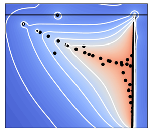
  $Ri_{\delta ^*} = 0.001$ shown in figure 2. All flows are stable, but the inclusion of thermal effects introduces additional modes compared with the Blasius case. These additional modes are related to the inclusion of the energy equation. In other words, when choosing a non-vanishing Richardson number, the modes related to the energy equation become relevant to the system dynamics due to its coupling with the momentum equation. Increasing the Prandtl number also adds more eigenvalues to the discrete spectrum, as can be observed when comparing the spectra in figures 3(b) and 3(c). The two least stable frequencies observed in these figures are located at $\omega _r \approx 0.4$ and $1.0$, where the latter is associated with the approximate representation of the continuous modes in the discrete spectra. When two-dimensional disturbances are excited on both Blasius and mixed convection boundary layers, the flows become unstable to Tollmien–Schlichting (TS) waves. In the present spectra, the TS waves are represented by the eigenvalues at $\omega _r \approx 0.4$.

Figure 3. Eigenspectra and pseudospectra for Blasius boundary layer (a) and mixed convection boundary layers with  $Pr = 0.7$ (b) and $Pr = 7.0$ (c). For all cases, $Re_{\delta ^*}=450$, $k_{\delta ^*}=0.31$ and $m_{\delta ^*}=0.0$. For the heated cases, $Ri_{\delta ^*}=0.001$. The eigenvalues are represented by the black circles while the pseudospectra are represented by the contours and isolines plotted in logarithmic scale. All pseudospectra plots are shown with the same levels.
The eigenvectors of the TS waves as well as the first, second and fifth least stable modes of the continuous spectrum are shown in figure 4, which also includes a thin grey horizontal line to highlight the hydrodynamic boundary layer thickness. Furthermore, all results are normalized to one for comparison purposes. Figure 4(a–c) presents results for the Blasius and mixed convection flows with  $Re_{\delta ^*}=450$, $k_{\delta ^*}=0.31$ and $m_{\delta ^*}=0.0$, where $Ri_{\delta ^*}=0.001$ for the heated cases. They indicate that the spatial support of the $u$ and $w$ velocity components is identical for the Blasius and heated cases. The latter, however, have non-negligible thermal disturbances with similar shapes, but a different wall-normal support that depends on the thermal boundary layer thickness. Continuous modes are displayed in figure 4(d–f) for $Re_{\delta ^*}=450$, $k_{\delta ^*}=0.31$, $m_{\delta ^*}=0.0$, $Ri_{\delta ^*}=0.001$ and $Pr = 7.0$. They indicate a spatially oscillatory behaviour in the wall-normal direction that spans the entire domain, except near the wall where they are negligible. As discussed by Grosch & Salwen (Reference Grosch and Salwen1978) and Zaki & Durbin (Reference Zaki and Durbin2021), the continuous modes can be associated with external disturbances that impact bypass transition in the boundary layer.

Figure 4. Magnitude of normalized eigenvectors of the (a–c) TS wave computed for  $Re_{\delta ^*}=450$, $k_{\delta ^*}=0.31$ and $m_{\delta ^*}=0.0$ for the Blasius and mixed convection boundary layers, with $Ri_{\delta ^*}=0.001$ for the heated cases, as well as (d–f) first (solid blue line), second (solid black line) and fifth (solid green line) least stable continuous modes for $Pr = 7.0$, $Re_{\delta ^*}=450$, $k_{\delta ^*}=0.31$ and $m_{\delta ^*}=0.0$, and $Ri_{\delta ^*}=0.001$. The thin grey horizontal lines highlight the boundary layer thickness.
A modal analysis provides insights into the disturbance time-asymptotic behaviour. However, the behaviour of linear disturbances in boundary layers is highly non-normal, i.e. the eigenvectors of the linear operator are not orthogonal (Andersson et al. Reference Andersson, Berggreen and Henningson1999; Schmid & Henningson Reference Schmid and Henningson2000). In such cases, a non-modal analysis provides insights into the disturbance transient behaviour (Schmid Reference Schmid2007; Schmid & Brandt Reference Schmid and Brandt2014). These non-normal effects are quantified here through the pseudospectra, which are also shown in figure 3 as colour contours delimited by white isolines. The levels are plotted in logarithmic scale. Such an analysis indicates which disturbances are the most sensitive to forcing as well as their response characteristics for the present two-dimensional modes. One can observe in this figure that non-normal effects are more pronounced between the most stable modes of the discrete spectrum and the continuous spectrum. Since the isoline levels are the same for all plots, it is possible to see that the pseudospectra of the Blasius and the mixed convection boundary layer with  $Pr=0.7$ have a similar topology. However, the latter is noticeably different near the least stable eigenvalue of the continuous spectrum at $\omega _r \approx 1.0$. This region of the spectrum shows strong interactions between multiple modes for the heated case. When the Prandtl number is increased to $Pr=7.0$, one can observe that the non-normal effects are more pronounced along the entire spectrum. This indicates that, for the same thermal conditions, the flow becomes more susceptible to external excitations at higher Prandtl numbers.
4.2. Resolvent and input–output analyses
In order to better understand the role played by external disturbances, the resolvent analysis is performed in a componentwise input–output form by choosing appropriate  $\boldsymbol{\mathsf{B}}$ and $\boldsymbol{\mathsf{C}}$ operators in (3.7) (see Schmid (Reference Schmid2007) for more details). The dominant terms from this analysis are shown in figure 5, where the curves are interpreted as ‘forcing’ $\rightarrow$ ‘response’. Figure 5(a–c) shows the cases with $Re_{\delta ^*}=510$. From left to right, the Blasius boundary layer, and the thermal cases evaluated at $Ri_{\delta ^*}=0.0001$ for $Pr = 0.7$ and $Pr = 7.0$ are shown. Figure 5(d–f) presents results for $Re_{\delta ^*}=450$, $Pr=7.0$ and different Richardson numbers, namely $Ri_{\delta ^*}=0.0001$ and $0.001$. All the cases presented in figure 5 are evaluated at $k_{\delta ^*}=0.31$ and $m_{\delta ^*}=0.0$. The gains of the resolvent operator are also depicted in figure 5(d) for all cases analysed. Under the conditions analysed, it is possible to assess the individual effects of Reynolds, Prandtl and Richardson numbers on the flow response to specific disturbances. Hence, the impact of inertial, shearing and buoyancy mechanisms can be evaluated.

Figure 5. Input–output analysis (‘forcing’  $\rightarrow$ ‘response’) and gains of the resolvent operator for different flow conditions excited by two-dimensional disturbances. All cases are solved for $k_{\delta ^*}=0.31$ and $m_{\delta ^*}=0.0$.
In the Blasius boundary layer, i.e. case 1, the largest receptivity occurs due to forcing of streamwise  $u$ and wall-normal $w$ velocity components. At the frequency of the TS waves, $\omega _r \approx 0.4$, forcing of $u$ leads to higher receptivity of $u$ and $w$, respectively. On the other hand, the receptivity roles played by streamwise and wall-normal components switch order in both forcing and response at the frequency of the continuous spectrum at $\omega _r \approx 1.0$. The dominant TS wave receptivity amplitudes are similar when mixed convection is considered at the same Reynolds number, independent of the Prandtl number. On the other hand, as expected from the results in figure 3, there is a considerable increase in the receptivity amplitude associated with the dominant continuous mode due to thermal effects. Cases 2 and 3 in figure 5 show that this occurs because thermal energy is converted into kinetic energy. In other words, there is a strong response from the streamwise and wall-normal velocity disturbance components to temperature disturbance forcing. Moreover, these cases also show that thermal receptivity to forcing by a temperature disturbance is more pronounced along the entire frequency spectrum for the higher Prandtl number considered here.
A comparison between cases 3 and 4 allows an assessment of inertia effects for the same thermal conditions. First and foremost, a change in Reynolds number only affects the receptivity mechanism associated with the dominant TS wave. Furthermore, its amplitude decreases with a reduction in Reynolds number, which is expected since figure 2 indicates that the discrete spectrum becomes even more stable. Finally, an analysis of the thermal effects can be made by comparing cases 4 and 5, which have the same Reynolds and Prandtl numbers, but different Richardson numbers. Receptivity amplitudes increase for both the TS wave at  $\omega _r \approx 0.4$ and the continuous mode at $\omega _r \approx 1.0$ when the Richardson number increases. Nevertheless, the latter is still dominant. For all input–output plots, one can also see the thermal response to $u$ velocity disturbances. Although this receptivity mechanism is not dominant when compared with the others, one can still see a Prandtl number effect. Larger temperature responses are observed between the two resonant peaks for case 2, which has a lower Prandtl number. Since this mechanism represents a transfer of kinetic to thermal energy, it is impacted by the temperature and velocity gradients of the boundary layers. The more similar profiles of the thermal and hydrodynamic boundary layers for $Pr = 0.7$ seem to enhance the present energy transfer mechanism. Finally, the gains of the resolvent operator are plotted for all cases. They confirm the higher amplification at $\omega _r \approx 1.0$ of case 5 due to an increase in thermal effects associated with a decrease in inertia effects. In other words, natural convection is strengthened while forced convection is weakened. Cases 2, 3 and 4 display similar gains for the dominant continuous mode. This implies that it is amplified the most by thermal effects, and slightly by shearing effects. On the other hand, the TS waves are amplified the most by inertial effects.
In order to provide further insight into the most relevant energy transfer mechanisms observed in the input–output analysis, the spatial support of the dominant forcing and response modes is analysed. Doing so, however, is not straightforward because the continuous mode far-field boundary conditions in the domain-truncated wall-normal direction are unknown and must be approximated. Although the results presented so far do not change for different far-field boundary conditions and domain sizes, as discussed in Appendices A and B, this is not the case for the far-field spatial support of the dominant forcing and response modes. Hence, in order to obtain interpretable results near the wall, the formulation proposed by Nogueira et al. (Reference Nogueira, Cavalieri, Hanifi and Henningson2020) is employed. It uses the integration weights of the inner product definition to remove the far-field support from the response modes in the resolvent analysis, leaving the forcing modes free along the entire domain. The weighting function proposed by Nogueira et al. (Reference Nogueira, Cavalieri, Hanifi and Henningson2020) consists of a hyperbolic tangent function with the following format:
 \begin{equation} W(z) = 0.5(1-b)\left[1-\tanh{(z_p-z)}\right]+b { ,} \end{equation}
where  $z_p$ stands for the cut-off height and $b$ is selected as $10^{-20}$ to avoid zero weighting for $z>z_p$. In this work, $z_p$ was evaluated with $7$ and $10\delta$. The former value approximately corresponds to the maximum wall-normal distance reached by the TS wave response modes, whereas the latter value was chosen to evaluate the influence of $z_p$ in the forcing/response modes of the continuous spectrum. The weighting function defined in (4.1) can be combined with (3.9) to yield
 \begin{equation} \tilde{\boldsymbol{\mathsf{L}}}_W = \boldsymbol{\mathsf{W}}\tilde{\boldsymbol{\mathsf{L}}}_E { ,} \end{equation}
where  $\boldsymbol{\mathsf{W}} = (\textrm {diag}(W,W,W,W,0))^{1/2}$. This new weighted operator can be directly applied to the input–output norm defined in (3.7) by replacing $\tilde {\boldsymbol{\mathsf{L}}}_E$ with $\tilde {\boldsymbol{\mathsf{L}}}_W$. Further discussion about weighting of the forcing and response modes is provided in Appendix C.
Figure 6 shows the spatial support of the dominant normalized forcing and response modes obtained using the above procedure for  $\omega =0.4$ (first two columns) and $1.0$ (last two columns) when $Re_{\delta ^*}=450$, $k_{\delta ^*}=0.31$ and $m_{\delta ^*}=0.0$, with $Ri_{\delta ^*}=0.001$ as well as $z_p=7$ and $10\delta$ for the heated cases. In the former case, related to TS waves ( $\omega =0.4$), the dominant forcing $\rightarrow$ response pairs are $u\rightarrow u$ and $u\rightarrow w$, as shown in the input–output maps of figure 5. There is essentially no difference between the Blasius and mixed convection cases, indicating that heating has no effect on either forcing or response mode support. Furthermore, forcing near the wall leads to a response both inside and outside of the boundary layer. Figure 5 also shows that the latter case, related to the continuous spectrum ( $\omega =1.0$), has $\theta \rightarrow u$ and $\theta \rightarrow w$ as the dominant forcing $\rightarrow$ response pairs. This indicates the presence of a thermal to kinetic energy transfer mechanism. Their spatial support is also shown in figure 6. It is possible to observe that such modes are not excited for the Blasius boundary layer case. This is an expected result, since setting $Ri_{\delta ^*}=0$ decouples the momentum and energy equations. On the other hand, they are significantly affected by heating, but only away from the wall. This is also expected, since the continuous spectrum eigenvectors display a spatial support along the entire wall-normal domain away from the wall as well, as shown in figure 4. Such a behaviour suggests that the unstably stratified boundary layer is susceptible to free-stream thermal disturbances, which can potentially impact bypass transition. Furthermore, the response mode support also indicates that the resulting flow structures are two-dimensional, like TS waves but with a larger support in the wall-normal direction. In other words, they are equivalent to the traditional transverse rolls that form Rayleigh–Bénard convection cells, but now in an unbounded domain. Finally, it is important to note that there is a significant difference between the $z_p=7$ and $10\delta$ results in the latter case. This is due to the fact that the continuous modes become non-normal when heated from below, allowing their superposition to generate a far-field spatial support in the dominant forcing and response modes. Hence, it becomes impossible to accurately isolate near-wall effects with the weighting function.

Figure 6. Magnitude of the dominant forcing and response modes computed for  $Re_{\delta ^*}=450$, $k_{\delta ^*}=0.31$ and $m_{\delta ^*}=0.0$, with $Ri_{\delta ^*}=0.001$ for the heated cases. The first (last) two columns show the modes calculated for $\omega =0.4$ ( $\omega =1.0$).
5. Conclusions
In this work, modal and non-modal analyses of shear flows including thermal effects are employed to assess the role of inertia, shear and buoyancy in unstably stratified horizontal boundary layers under a regime of mixed convection. The flows are modelled by the incompressible Navier–Stokes equations including the OB approximation, which couples the energy and momentum equations through buoyancy effects. The stability properties of two-dimensional disturbances are investigated by a modal analysis to identify the onset of instability. Results are presented in terms of the neutral curves for the Blasius boundary layer (without thermal effects) and for several cases of mixed convection, where the roles of the Prandtl and Richardson numbers are evaluated. It is shown that both these non-dimensional parameters destabilize the flow. However, the Richardson number has a more pronounced effect in reducing the critical Reynolds number.
A resolvent analysis is applied to understand the system's response to forcing near marginal stability parametric conditions. Within such a framework, non-normality effects of the linear operator are investigated. Considering the same Reynolds number, the spectra and pseudospectra are presented for the Blasius boundary layer and for two heated boundary layers with different Prandtl numbers, but the same Richardson number. Results show that both the inclusion of thermal effects and the increase in the Prandtl number lead to the emergence of additional discrete modes in the spectrum. Changes in the Prandtl number also lead to different topologies in the pseudospectra. The resolvent formalism is also employed in a componentwise input–output approach to investigate the flow response to specific forcing disturbances. In such analysis, an evaluation of the inertial, shearing and buoyancy mechanisms is possible through variations in the Reynolds, Prandtl and Richardson numbers. Results demonstrate that the Richardson number has a great impact in the thermal to kinetic disturbance energy conversion, leading to a strong amplification of the flow response for the least stable mode of the continuous spectrum due to non-normality effects. On the other hand, the Reynolds number is shown to affect only the stability properties of TS waves, while the Prandtl number affects mostly the response in terms of temperature fluctuations between resonances.
These results were obtained using Dirichlet boundary conditions in the far field, which are arguably the most commonly employed boundary conditions for local stability analyses in semi-infinite domains. Although this choice is an adequate one for the computation of discrete modes, this is not the case for their continuous counterparts. As far as the authors are aware, however, the correct artificial boundary conditions for continuous modes in a truncated semi-infinite domain are not known, except in some highly simplified problems. All that is known is that these modes and their derivatives are bounded in the far field. This is not a significant issue for the Blasius boundary layer because the continuous modes are normal. Things change when heating is applied because they become strongly non-normal. For this reason, result sensitivity to the artificial far-field boundary model employed was analysed in three different ways, namely (i) using Neumann boundary conditions as well, (ii) using three different domain sizes and (iii) using a weighting function in the resolvent operator that filters out the far-field behaviour of the response modes. None of the results presented were significantly altered when using these different far-field boundary models because they are constrained to the near-wall region. There is only one exception. The spatial support of the weighted forcing and response modes associated with the continuous spectrum under heating depends on the filter cut-off height. This is due to the fact that the unstably stratified boundary layer is strongly susceptible to free-stream thermal disturbances, which can potentially impact bypass transition. Nevertheless, it is possible to notice that the structure of the response mode is analogous to the transverse rolls typically found in Rayleigh–Bénard convection, but now with a larger support in the wall-normal direction due to its unbounded nature. Direct numerical simulations could shed light into the role of these structures. They could also be used to further explore the thermal to kinetic energy transfer mechanism in heated boundary layers as a means of flow control. These are suggested here for future investigations.
Acknowledgements
The authors thank Dr T.R. Ricciardi for fruitful discussions during the course of this work.
Funding
The authors acknowledge Fundação de Amparo à Pesquisa do Estado de São Paulo, FAPESP, for supporting the present work under research grant nos. 2013/08293-7, 2021/06448-0 and 2022/00464-6, and Conselho Nacional de Desenvolvimento Científico e Tecnológico, CNPq, for supporting this research under grant nos. 407842/2018-7, 304335/2018-5 and 435413/2018-0.
Declaration of interests
The authors report no conflict of interest.
Appendix A. Result sensitivity with respect to far-field boundary conditions
In order to demonstrate the robustness of the results provided in this paper, a result sensitivity analysis is performed in this and the following appendices. The present one does so with respect to the far-field boundary conditions applied at the truncated unbounded domain in the wall-normal direction. Several authors (Schmid & Henningson Reference Schmid and Henningson2000; Nogueira et al. Reference Nogueira, Cavalieri, Hanifi and Henningson2020; Parente et al. Reference Parente, Robinet, De Palma and Cherubini2020) employ Dirichlet boundary conditions  $(\hat {\boldsymbol {q}}=0)$ in the far field when performing a local stability analysis on semi-infinite domains. While this type of boundary condition is an adequate one for computing the discrete modes of the spectrum, it is not accurate for the computation of their continuous counterparts. As discussed by Grosch & Salwen (Reference Grosch and Salwen1978) and Zaki & Durbin (Reference Zaki and Durbin2021), the continuous modes are not necessarily zero in the far field, but bounded instead. This is the motivation of the present analysis, which compares the eigenspectra and pseudospectra obtained while using Dirichlet and Neumann boundary conditions at the far-field artificial boundary.
Such a comparison is performed for the mixed convection boundary layer with  $Re_{\delta ^*}=450$, $Ri_{\delta ^*}=0.001$, $Pr_{\delta ^*}=0.7$, $k_{\delta ^*}=0.31$ and $m_{\delta ^*}=0.0$. Results are shown in figure 7 for Dirichlet (figure 7a) and Neumann (figure 7b) boundary conditions, i.e. $\hat {\boldsymbol {q}}=0$ and $\partial \hat {\boldsymbol {q}}/\partial z=0$, respectively. Both spectra and pseudospectra are graphically identical. In other words, both boundary conditions lead to essentially the same modal and non-modal results. Although neither boundary condition is the correct one for the artificially truncated far-field boundary, the above results provide some evidence that the present linear stability analysis is robust with respect to the far-field boundary condition choice.

Figure 7. Eigenspectra and pseudospectra computed for the mixed convection boundary layer with  $Re_{\delta ^*}=450$, $Ri_{\delta ^*}=0.001$, $Pr_{\delta ^*}=0.7$, $k_{\delta ^*}=0.31$ and $m_{\delta ^*}=0.0$ employing the Dirichlet (a) and Neumann (b) boundary conditions in the far field.
Appendix B. Result sensitivity with respect to domain size
This second appendix evaluates result sensitiveness with respect to the wall-normal domain size. Results are shown in figure 8 for the same parametric conditions used to evaluate figure 7, where the imposed domain height  $z_{max}$ is $10 \delta$ (figure 8a), $30 \delta$ (figure 8b) and $50 \delta$ (figure 8c). The latter two figures are essentially identical, but the former ones displays some small differences. In this smaller domain size ( $z_{max} = 10 \delta$), the discrete modes of the spectrum are well resolved, but the lower portion of the continuous spectrum does display some differences with respect to the larger domains. Since the modal and non-modal results presented in this paper were obtained with $z_{max} = 30 \delta$, they can be considered as independent of domain size.

Figure 8. Eigenspectra and pseudospectra computed for the mixed convection boundary layer with  $Re_{\delta ^*}=450$, $Ri_{\delta ^*}=0.001$, $Pr_{\delta ^*}=0.7$, $k_{\delta ^*}=0.31$ and $m_{\delta ^*}=0.0$, employing the Dirichlet boundary condition with different domain sizes.
Appendix C. Result sensitivity with respect to weighting function
Finally, this third and final appendix evaluates result sensitiveness with respect to the weighting function employed to filter out the far-field support of the response modes from the receptivity analysis. Results are shown in figure 9 for the same parametric conditions used to evaluate figures 7 and 8, including the dominant forcing and response modes calculated at  $\omega =0.4$ (first two columns) and $\omega =1.0$ (last two columns). One can observe that the TS dominant forcing and response modes are graphically identical, independent of the far-field boundary condition and weighting function employed. On the other hand, the far-field artificial boundary conditions have a significant impact on the spatial support of the continuous modes. This is expected since the continuous-mode eigenvectors exist in the free stream and are not constrained to the near-wall region. While the Dirichlet boundary condition requires that the eigenvectors decay to zero in the far field, the Neumann do so for their wall-normal derivatives. This change causes noticeable differences in the support of the forcing and response modes for $\theta \rightarrow w$. However, their $\theta \rightarrow u$ counterparts remain graphically identical. The inclusion of a weighting function, following the approach from Nogueira et al. (Reference Nogueira, Cavalieri, Hanifi and Henningson2020), makes the continuous modes independent of boundary condition. This is an interesting observation that provides evidence in favour of this approach.

Figure 9. Magnitude of the dominant forcing and response modes computed for  $Re_{\delta ^*}=450$, $Pr_{\delta ^*}=0.7$, $k_{\delta ^*}=0.31$ and $m_{\delta ^*}=0.0$, with $Ri_{\delta ^*}=0.001$ for the heated cases. They were computed for Dirichlet $(\hat {\boldsymbol {q}}=0)$ and Neumann $(\partial \hat {\boldsymbol {q}}/\partial z=0)$ boundary conditions with and without the weighted modes; the former denoted by $\boldsymbol{\mathsf{W}}$ (Nogueira et al. Reference Nogueira, Cavalieri, Hanifi and Henningson2020) and with $z_p=7\delta$. The first (last) two columns show the modes calculated for $\omega =0.4$ ( $\omega =1.0$).


