


1. Introduction
A thermal plume is a common phenomenon of natural convection, which commonly exists in natural and industrial systems (e.g. mountainous climates, deep-sea hydrothermal vents, industrial chimneys). The plume develops due to the buoyancy effect, which may be induced by a temperature difference (Métivier, Li & Magnin Reference Métivier, Li and Magnin2017; Xu, Shi & Xi Reference Xu, Shi and Xi2019) or other processes. Many experimental, numerical and theoretical studies (List Reference List1982; Vincent, Yuen & Munqer Reference Vincent, Yuen and Munqer2012) of plumes have been performed due to their significance in fundamental research and engineering applications. Additionally, a plume may be influenced by the size (Guha & Sengupta Reference Guha and Sengupta2016), shape (Kondrashov, Sboev & Dunaev Reference Kondrashov, Sboev and Dunaev2016, Reference Kondrashov, Sboev and Dunaev2017) and heating method (Mellado Reference Mellado2012) of the source. Thus, the plume from a point, line or surface heat source is typically considered in many studies due to their simplicity of geometry (Rotem & Claassen Reference Rotem and Claassen1969; Fay Reference Fay1973; Hunt & Bremer Reference Hunt and Bremer2011).
Kozanoglu & Lopez (Reference Kozanoglu and Lopez2007) indicated that a thermal boundary layer may appear on a horizontal plate after the plate is heated. A horizontal convective flow may form in the thermal boundary layer due to the baroclinic effect, which is referred to as lapping flow (Hattori et al. Reference Hattori, Bartos, Norris, Kirkpatrick and Armfield2013). The thickness and velocity of the thermal boundary layer on an isothermal plate may be scaled with (κt)1/2 and κ 5/2t 3/2Ra/W 4 for t < ts (ts ~ W 2/(κRa 2/5)) but with κRa 2/5/W (Jiang, Nie & Xu Reference Jiang, Nie and Xu2019) and W/Ra 1/5 (Rossby Reference Rossby1965) for t > ts. Here, Ra is the Rayleigh number, κ is thermal diffusivity, W is the plate length, t is time, and ts is the critical time after which the thermal boundary layer does not grow up at an equilibrating state between convective and conductive heat transfer.
The convective flow merges in the middle of the plate, resulting in the appearance of a starting plume (Turner Reference Turner1962), which typically involves a cap and a stem (Torrance, Orloff & Rockett Reference Torrance, Orloff and Rockett1969). Thus, a variety of phenomena, such as the buoyant blob, the mushroom cap and the buoyant vortex ring, occur in the starting plume, as described by Atkinson & Davidson (Reference Atkinson and Davidson2019). As time passes, the cap may develop and even break (Shlien Reference Shlien1978; Rogers & Morris Reference Rogers and Morris2009). Only one starting plume can form if the size of the heated plate is small; however, multiple starting plumes can appear on a heated horizontal plate if the size of the plate is larger than the size of the plumes (Sparrow, Husar & Goldstein Reference Sparrow, Husar and Goldstein1970). Early laboratory studies (e.g. Shlien Reference Shlien1976; Moses, Zocchi & Libchaber Reference Moses, Zocchi and Libchaber1993; Olson, Schubert & Anderson Reference Olson, Schubert and Anderson1993) measured the temperature and velocity of the starting plume. Kaminski & Jaupart (Reference Kaminski and Jaupart2003) characterized the dependence on the Prandtl number of the starting plume and indicated that the development of the starting plume may involve a conductive stage, a velocity increase stage, a plateau stage, where the plume velocity is constant, and a velocity decrease stage. The velocity of the plume in the plateau stage may also be scaled with (gβq/ρνcp)1/2, where g is the acceleration due to gravity; β is the coefficient of thermal expansion; q is the power input; ρ is the density; ν is the kinematic viscosity and cp is the heat capacity. Davaille et al. (Reference Davaille, Limare, Touitou, Kumagai and Vatteville2011) also demonstrated that there is a Gaussian distribution of the velocity in the plateau stage and indicated that the difference in the experimental rig, the working fluid and the size of the tank may result in the difference in the velocity distribution. Additionally, Jiang et al. (Reference Jiang, Nie and Xu2019) showed that the velocity of the starting plume on an isothermal horizontal plate may be scaled with Raκ 7/3t 4/3/W 11/3 in the velocity increase stage but with Ra 7/15κ/W in the plateau stage.
The plume could be laminar or even turbulent (Bhamidipati & Woods Reference Bhamidipati and Woods2017). Batchelor (Reference Batchelor1954) presented the classical theory of the steady laminar plume. The experimental and numerical results have also well characterized the laminar plume (Kondrashov & Burkova Reference Kondrashov and Burkova2018). With an increase in the governing parameters (e.g. the Rayleigh number), the plume on the horizontal plate may become unstable (Chen & Tzuoo Reference Chen and Tzuoo1982); thus, once the Rayleigh number increases beyond a critical value, a steady plume on the plate may become periodic with a puffing mode (Khrapunov & Chumakov Reference Khrapunov and Chumakov2020). The experiment recorded and verified the presence of such a puffing mode (Hattori et al. Reference Hattori, Bartos, Norris, Kirkpatrick and Armfield2013). Additionally, a flapping mode can also be present in periodic plumes (Plourde et al. Reference Plourde, Pham, Kim and Balachandar2008). Puffing and flapping modes have been described in the governing parameter space (Hattori, Armfield & Kirkpatrick Reference Hattori, Armfield and Kirkpatrick2012). With an increase in the Rayleigh number, the plume on the horizontal plate may transition from a laminar to a turbulent state (Lopez & Marques Reference Lopez and Marques2013; Khrapunov & Chumakov Reference Khrapunov and Chumakov2020); thus, the plume on the horizontal plate may become turbulent when the Rayleigh number is sufficiently large (Theerthan & Arakeri Reference Theerthan and Arakeri2000; Vouros & Panidis Reference Vouros and Panidis2012). The experiment of Theerthan & Arakeri (Reference Theerthan and Arakeri2000) confirmed the existence of line plumes in the turbulent convective flow. These line plumes seem to be aligned diagonally, due to the large-scale flow. Also, the contraction and repulsion regimes of the turbulent plume have been investigated by Plourde et al. (Reference Plourde, Pham, Kim and Balachandar2008) and Vouros & Panidis (Reference Vouros and Panidis2012).
Plumes on heating sources with complex geometries, such as open cavities, have also been studied due to their common presence in natural and industrial systems. Townsend (Reference Townsend1959) performed the first experiment on a plume on an open box with a heated bottom in which the horizontal shear effect was observed. Hasnaoui, Bilgen & Vasseur (Reference Hasnaoui, Bilgen and Vasseur1990) and Saxena et al. (Reference Saxena, Kishor, Singh and Srivastava2018) indicated that a plume on the groove with a heated bottom may undergo a pitchfork bifurcation when symmetry is broken. A succession of bifurcations may occur in the transition of the plume on the groove, which has been characterized based on numerical and experimental results by Qiao, Xu & Saha (Reference Qiao, Xu and Saha2018b), Qiao et al. (Reference Qiao, Tian, Yang and Xu2020) and Qiao, Gao & Xu (Reference Qiao, Gao and Xu2021).
Because an open cylinder has a unique geometry and is common in nature (e.g. a pan on a stove, a hot crater), a plume on an open cylinder has also been studied. The experimental study of Lewandowski, Bieszk & Cieslinski (Reference Lewandowski, Bieszk and Cieslinski1992) indicated that the heat transfer of a fully developed plume on an open cylinder is dominated by the screening effect (H/D < 0.08) and the chimney effect (H/D > 0.08), where H and D are the height and diameter of the cylinder, respectively. Recently, Qiao et al. (Reference Qiao, Tian, Nie and Xu2018a) and Zhang et al. (Reference Zhang, Qiao, Nie and Xu2021) reported that the fully developed plume on the open cylinder could tilt in any direction of the sidewall after the breaking of the axial symmetry, dependent on perturbations, and a transition route from a steady to chaotic state has been characterized. Interestingly, the fully developed plume on an open cylinder may undergo a reverse bifurcation from a periodic to steady state, which is referred to as a period bubbling bifurcation (Zhang et al. Reference Zhang, Qiao, Nie and Xu2021). The numerical results that were obtained but not presented by Qiao et al. (Reference Qiao, Xu and Saha2018b) also demonstrated that the transition route to chaos of the fully developed plume is dependent on the aspect ratio of the open cylinder. Although the fully developed plume on an open cylinder has been described, theoretical and experimental studies of the transient plume on the cylinder remain rare. In particular, the dynamic evolution and scaling laws under different regimes of the transient circular column plume on the open cylinder after sudden heating below remain unknown, and the transition route to chaos of the fully developed plume must be characterized and verified in the experiment. Accordingly, we performed a simple scaling analysis for the transient circular column plume on an open cylinder and a set of experiments using a shadowgraph for flow visualization and a thermistor for temperature measurement.
In the remainder of this paper, we describe the experimental set-up in § 2; present a simple scaling analysis for a transient plume on an open cylinder in § 3; characterize the plume on an open cylinder from the developing to fully developed stage in § 4 and summarize the conclusions in § 5.
2. Experimental set-up
2.1 Experimental apparatus
In this study, we built an experimental apparatus involving an open cylinder with an inner diameter D = 15 mm and height H = 7.5 mm that was placed at the centre of the bottom of the tank with inner dimensions of 300 mm × 300 mm × 300 mm, as shown in figure 1(a). An aspect ratio of H/D = 0.5 was selected in the experiment based on a number of numerical tests; thus, diverse bifurcations exist for such a fixed aspect ratio (Zhang et al. Reference Zhang, Qiao, Nie and Xu2021). The open cylinder was built with a 3-mm-thick Perspex plate for the sidewall but with a 3-mm-thick cylindrical copper plate for the bottom wall, as shown in figure 1(b). The tank containing water as the working fluid was built with 10-mm-thick Perspex plates for the top and sidewalls but with a 15-mm-thick Perspex plate for the bottom wall to reduce the heat transfer through the bottom wall from the water bath.

Figure 1. (a) Schematic of the experimental set-up, (b) a photo image of an open cylinder and (c) a zoom-in on the water bath in panel (a).
A constant temperature water bath with inner dimensions of 30 mm × 30 mm × 30 mm was mounted under the copper plate of the cylinder for heating, as shown in figure 1(c). The water bath was connected to the circulator (BILON-GDW-3001AS with a temperature accuracy of 0.01 K) through a water inlet (inner diameter of 16 mm) and two water outlets (inner diameter of 10 mm). The hot water may be poured into the water bath through the water inlet and out back to the circulator through the water outlet. Such a circulating system may be used to keep a specified temperature for the bottom wall of the cylinder. In this study, the section area of the water outlet is slightly smaller than that of the water inlet so that the water bath is fully filled with hot water.
The thermal conductivity of the Perspex plates (0.15 W m−1 K−1) is much lower than that of the copper plate (401 W m−1 K−1), and thus, the heat flux through the Perspex plates is considered negligible in this study. Further, the Perspex wall may be considered adiabatic, as in previous studies (Patterson et al. Reference Patterson, Graham, Schöpf and Armfield2002; Xu, Patterson & Lei Reference Xu, Patterson and Lei2008). Additionally, because the 15-mm-thick Perspex plate was used for the bottom wall of the tank, which is thicker than the other walls, the heat transfer through the bottom wall of the water tank from the water bath is even lower.
Flow visualization was performed using a shadowgraph system, as shown in figure 2. In the shadowgraph system, two spherical mirrors with diameters of 300 mm were placed on two sides of the tank, and a point source of light was located at the focus of one spherical mirror but a digital camera at that of the other spherical mirror. A beam of light was first emitted from the point source of light to the left spherical mirror in figure 2, and then, a parallel light from the left spherical mirror was reflected to the tank. Because the variance in the temperature of the water may lead to the variance in the density and thus water's refractive index, the parallel light is refracted when it passes through the water in the tank. The refracted light is reflected on the digital camera by the spherical mirror conversely, and thus, the shadowgraph image characterizing the fluid flow can be recorded.

Figure 2. Schematic of a shadowgraph system.
Figure 3 shows shadowgraph images before and during the experiment. The section of the open cylinder on the bottom of the tank is dark in the shadowgraph image in figure 3(a) because the parallel light was refracted away due to the bend of the sidewall of the cylinder. Thus, the fluid flow in the open cylinder cannot be visualized in the experiment. A coordinate system was set at the centre of the bottom of the open cylinder in figure 3(a), which is used in the study.

Figure 3. (a) Shadowgraph image before the experiment. (b) Shadowgraph image of a starting plume at t = 17 s for Ra = 8.81 × 10⁵ (ΔT = 15 K).
A starting plume is shown at t = 17 s for Ra = 8.81 × 10⁵ in figure 3(b). The starting plume comprises a cap, a lobe and a stem. In this study, the cap forms due to the obstruction of the ambient fluid when the starting plume rises, during which the ambient fluid is continuously entrained into the cap. With increasing time, the cap of the plume becomes larger and the lobe of the plume becomes longer. Heat transfer through the Perspex bottom wall can occur, albeit small, and thus result in small perturbations outside the cylinder, as shown in figure 3. Further examination of the experimental results shows that such perturbations outside the cylinder are weak and may be considered negligible in the plume above the cylinder.
In the experiment, the thermistor (GAG22K7MCD419) and the data acquisition system (Keithley 2700 multimeter) were applied for temperature measurement (accuracy of 0.01 K). Six identical thermistors were located at different points, including the point (0, 0, 0.75 mm) adjacent to the bottom of the cylinder; the point (0, 0, 7.5 mm) at the outlet of the open cylinder; the point (0, 0, 150 mm) at the centre of the tank; and the other two points (10 mm, 0, 150 mm) and (−10 mm, 0, 150 mm), as shown in figure 3(a). The origin of the coordinate axis is at the centre of the bottom of the open cylinder, as shown in figure 3(a). In addition, the thermistor was also mounted under the copper plate for temperature measurement in the water bath.
2.2 Experimental procedures
The water in the tank remained quiescent and the temperature was T 0 before each experiment. Once the experiment started up, the hot water with the specified temperature was transported from the circulator to the water bath so that sudden heating was set up on the bottom of the cylinder with the heating temperature Th. In this study, the heating temperature difference is ΔT = Th − T 0. The three dimensionless governing parameters determining the thermal plume are the Rayleigh number Ra, the Prandtl number Pr and the aspect ratio A, respectively, and are defined as
 \begin{gather}Ra = \frac{{g\beta \Delta T{D^3}}}{{\nu \kappa }},\end{gather}
 \begin{gather}Pr = \frac{\nu }{\kappa },\end{gather}
 \begin{gather}A = \frac{H}{D},\end{gather}
where g, β, v and κ are gravity acceleration, coefficient of thermal expansion, kinematic viscosity and thermal diffusivity, respectively.
In this study, a series of experiments with seventeen temperature differences between the water at the initial time and the bottom wall of the open cylinder were performed, as shown in table 1. The initial temperature of the water in the tank ranges from 296.95 to 299.35 K, for which the minimum temperature difference is 2 K, and the maximum temperature difference is 40 K. The corresponding Rayleigh and Prandtl numbers range from 1.18 × 10⁵ to 2.34 × 10⁶ and 6.01 to 6.39, respectively. The aspect ratio is fixed at A = 0.5 in this study. The uncertainty of the experimental data is smaller than 3 %.
Table 1. Experimental parameters.

3. Scaling analysis
The convective flow on an open cylinder is driven by the buoyant force induced by the heated bottom wall but not by the sidewall. The comparison between the previous numerical results of Jiang et al. (Reference Jiang, Nie and Xu2019) and the experimental results also shows that the sidewall or aspect ratio of the open cylinder negligibly influences the dynamic evolution of the starting plume after sudden heating. Thus, the effect of the sidewall is neglected in the following scaling analysis. Clearly, a thermal boundary layer can first form on the bottom wall of the open cylinder after the bottom wall is suddenly heated, and the thickness of the thermal boundary layer increases with δ ~ (κt)1/2 (also see Patterson & Imberger Reference Patterson and Imberger1980). Once the thickness is larger than the critical value, the thermal boundary layer becomes unstable. Such an instability results in a baroclinity effect in the thermal boundary layer in which the horizontal temperature contours become inclined (Hattori et al. Reference Hattori, Bartos, Norris, Kirkpatrick and Armfield2013). The duration before the onset of the instability of the thermal boundary layer is possibly estimated based on the stability analysis of the thermal boundary layer in the open cylinder.
The baroclinity effect may drive the fluid in the thermal boundary layer to the centre of the bottom wall. The velocity of the horizontal convective flow may be scaled with u ~ κ 5/2t 3/2Ra/D 4, as reported by Jiang et al. (Reference Jiang, Nie and Xu2019). The diameter of the bottom wall (D) is selected as the characteristic length because the bottom wall is a heat source driving the convective flow. As time proceeds, the horizontal convective flow becomes stronger. Thus, the development of the thermal boundary layer may enter an equilibrating state at which the heat conducted from the bottom wall is completely convected away; thus, the thermal boundary layer on the bottom wall does not grow. The thickness and velocity in the equilibrating stage may be scaled with δs ~ D/Ra 1/5 (Rossby Reference Rossby1965) and us ~ κRa 2/5/D for t > ts (ts ~ D 2/(κRa 2/5)) (Jiang et al. Reference Jiang, Nie and Xu2019). In this study, ts is the critical time at which the convective flow enters the equilibrating stage.
The heated fluid is convected to and piles up at the centre of the bottom wall and in turn results in the appearance of a starting plume due to the buoyancy effect. As time increases, the plume rises and even is removed from the open cylinder, as shown in figure 3(b). The plume clearly originates from the thermal boundary layer, and thus, the flow rate of the circular column plume may be scaled with that of the thermal boundary layer:
 \begin{gather}Q \sim {\rm \pi}r_{p}^2{w_{p}} \sim {\rm \pi}Du\delta \sim
\left\{\matrix{{\dfrac{{{\rm \pi} {\kappa^3}{t^2}Ra}}{{{D^3}}}}, & \quad t < {t_s}, \cr {\rm \pi} \kappa DR{a^{1/5}}, & \qquad t \ge {t_s}}\right.\end{gather}
\begin{gather}Q \sim {\rm \pi}r_{p}^2{w_{p}} \sim {\rm \pi}Du\delta \sim
\left\{\matrix{{\dfrac{{{\rm \pi} {\kappa^3}{t^2}Ra}}{{{D^3}}}}, & \quad t < {t_s}, \cr {\rm \pi} \kappa DR{a^{1/5}}, & \qquad t \ge {t_s}}\right.\end{gather}where the subscript p denotes the plume and the subscript s denotes the equilibrating stage, which is approximately steady. Here, Q depends on the Rayleigh number and the diameter (D) of the open cylinder for t > ts, which is different from that for the horizontal plate (Q ~ κRa 1/5; see Jiang et al. Reference Jiang, Nie and Xu2019) because a circular bottom wall is considered in this study.
The plume is driven by the buoyant force (gβΔT) but dissipated by the viscous force  $(\nu {w_p}/r_p^2)$ and inertial force (wp/t). Thus, based on (3.1), we may obtain the velocity and radius scales of the circular column plume in the developing stage when buoyant and viscous forces are equal:
 \begin{gather}{w_{pv}} \sim \frac{{{\kappa ^2}tRa}}{{{D^3}}},\end{gather}
 \begin{gather}{r_{pv}} \sim \sqrt {\kappa{t}} ,\end{gather}
and when buoyant and inertial forces are equal:
 \begin{gather}{w_{pi}} \sim \frac{{{\kappa ^2}tPrRa}}{{{D^3}}},\end{gather}
 \begin{gather}{r_{\textit{pi}}} \sim \sqrt {\frac{{\kappa{t}}}{{Pr}}} ,\end{gather}
where the subscripts v and i denote buoyant viscous and buoyant inertial regimes, respectively.
We also have the ratio of the inertial force (wp/t) to viscous force  $(\nu {w_p}/r_p^2)$ to be $r_p^2/\nu t$ , which may be expressed based on (3.4) and (3.6):
 \begin{gather}\frac{{r_{pv}^2}}{{\nu t}} \sim \frac{1}{{Pr}},\end{gather}
 \begin{gather}\frac{{r_{pi}^2}}{{\nu t}} \sim \frac{1}{{P{r^2}}}.\end{gather}
The equations mean that the plume rises under a buoyant viscous regime for Pr > 1 but under a buoyant inertial regime for Pr < 1. In this study, the buoyant viscous regime may always dominate the plume because the working fluid is water (Pr > 1; see table 1).
Additionally, we may also obtain the velocity and radius of the plume in the equilibrating stage for t > ts. Thus, substituting ts ~ D 2/(κRa 2/5) into (3.3) and (3.4), respectively, we have
 \begin{gather}{w_{psv}} \sim \frac{{\kappa R{a^{3/5}}}}{D},\end{gather}
 \begin{gather}{r_{psv}} \sim \frac{D}{{R{a^{1/5}}}}.\end{gather}
The velocity and radius scales of the circular column plume are different from those of the plume based on the assumption of the two-dimensional plane proposed by Jiang et al. (Reference Jiang, Nie and Xu2019). Also, a circular column plume is common in natural and industrial systems. In the equilibrating stage, the heat flux of the circular column plume may be scaled with ρcpQsΔT/ ${\rm \pi}$D 2. Based on (3.2), we may normalize the heat flux using kΔT/D and thus obtain the Nusselt number (Nus):
 \begin{equation}N{u_s} \sim R{a^{1/5}},\end{equation}
which is consistent with the scaling law of the Nusselt number reported by Jiang et al. (Reference Jiang, Nie and Xu2019). The characteristic length defining Nus and Ra is the diameter of the bottom wall in this study.
The velocity, radius, time and flow rate may be non-dimensionalized using κRa 2/5/D, D, D 2/(κRa 2/5) and  ${\rm \pi}$κDRa 2/5, respectively. Thus, (3.1), (3.2), (3.3), (3.4), (3.9) and (3.10) can be expressed in the non-dimensional format:
 \begin{gather}{Q^ \ast } \sim R{a^{ - 1/5}}{\tau ^2},\end{gather}
 \begin{gather}Q_s^ \ast\sim R{a^{ - 1/5}},\end{gather}
 \begin{gather}{W_{pv}} \sim R{a^{1/5}}\tau ,\end{gather}
 \begin{gather}{R_{pv}} \sim R{a^{ - 1/5}}{\tau ^{1/2}},\end{gather}
 \begin{gather}{W_{psv}} \sim R{a^{1/5}},\end{gather}
 \begin{gather}{R_{psv}} \sim R{a^{ - 1/5}}.\end{gather}
Here, τ is the non-dimensional time; and Q*,  $Q_s^\ast $, Wpv, Wpsv, Rpv and Rpsv are the non-dimensional flow rates, non-dimensional velocities and non-dimensional radii in the developing and equilibrating stages, respectively. These non-dimensional quantities will be used in the following section for validation.
4. Experimental results and discussion
Figure 4 shows the development of the plume on an open cylinder after sudden heating for Ra = 1.77 × 10⁶, which may be divided into three stages (a developing stage, an equilibrating stage and a fully developed stage), as shown by the velocity of the plume. In this study, the non-dimensional time of τs ~ 4 (where τs = t/ts) is the time of the transition from the developing stage to the equilibrating stage in the experiment but not the unity proposed in the scaling analysis. This result occurs because the baroclinity effect appears, and thus, the convective flow appears only after the onset of instability of the thermal boundary layer, as described in the scaling analysis. Because the duration before the onset of the instability of the thermal boundary layer is not considered in the scaling analysis, the time of the transition to the equilibrating stage proposed in the scaling analysis is smaller than that in the experiment (also see Jiang et al. Reference Jiang, Nie and Xu2019 for numerical results). The duration before the onset of the instability of the thermal boundary layer may be estimated based on further stability analysis, which is, however, beyond the scope of this study.

Figure 4. Velocity of the plume front at different stages for Ra = 1.77 × 10⁶, where τ ~ 4 is the non-dimensional time of the transition to the equilibrating stage.
Additionally, the development of the plume inside the cylinder was not visualized due to the refraction of the parallel light by the sidewall of the cylinder, and thus, the velocity across a smaller time duration is not shown in figure 4. Also, the experimental results show that the equilibrating stage defined in the scaling analysis is a transient equilibrium; thus, as the starting plume moves away and the fluid in the tank is stratified with time, the plume slowly develops into the fully developed stage, as shown in figure 4. In the following section, the development of the plume will be further characterized and analysed at different stages.
4.1 Development of the plume in different stages
4.1.1 Developing stage
A starting plume appears on the cylinder after sudden heating. Figure 5 shows two sets of shadowgraph images of the starting plume at different times. As time increases, the cap of the plume becomes larger due to the blockage of the motionless ambient fluid, and the lobe of the plume becomes longer due to the action of shear force. At a smaller Rayleigh number, there is only one single plume in the early time, as shown in figure 5(a1–a5) for Ra = 1.18 × 10⁵. However, for the larger Rayleigh numbers (e.g. Ra = 2.34 × 10⁶), two or even three plumes appear concurrently and eventually merge together with a thicker stem, due to the entrainment around the rising plumes (Pera & Gebhart Reference Pera and Gebhart2006), as shown in figure 5(b1–b5). The experimental results indicate that the cap of the plume rises more quickly with increasing Rayleigh number. All plumes eventually tilt to the sidewall of the open cylinder in which the axial symmetry of the plume has broken.

Figure 5. Flow structure of the starting plume in the developing stage. (a1–a5) From t = 46 s with a time interval of 6 s for Ra = 1.18 × 10⁵ and (b1–b5) from t = 22 s with a time interval of 1.5 s for Ra = 2.34 × 10⁶.
As mentioned above, the starting plume is axisymmetric in the early time for the smaller Rayleigh number, and the axial symmetry breaks as the plume cap rises downstream. To characterize the break-up of axial symmetry, figure 6 shows the temperature at the point (0, 0, 7.5 mm) and the shadowgraph images at different times for Ra = 1.18 × 10⁵. The plume is approximately axisymmetric around τ = 3.28 but tilts to the sidewall around τ = 3.62, as shown in figure 6(a). The break-up of the axial symmetry of the starting plume results in a sudden drop in the temperature at approximately τ = 3.28 because the temperature monitoring point (0, 0, 7.5 mm) is located at the centre of the outlet of the cylinder at which the plume stem moves away and tilts to the sidewall, as shown in figure 6(a). Because the second plume cap appears around time τ = 5.53, the temperature also begins to rise again, as shown in figure 6(b). Thus, the temperature at the downstream point near the top-open cylinder exhibits an oscillatory increase with time in the early stage because the more heated fluid and the hotter fluid from the proximity of the bottom wall may be convected further downstream as time increases in the early stage, which is also perturbed by multiple plume fronts in figures 6(a) and 6(b).

Figure 6. Flow structure of the starting plume and the temperature at the point (0, 0, 7.5 mm) in the developing stage for Ra = 1.18 × 10⁵. (a,b) Shadowgraph images at different times.
The critical time of the break-up of the axial symmetry of the plume is dependent on the Rayleigh number. To quantify the break-up of the axial symmetry of the plume, we also measured the time (τas) at the occurrence of the break-up based on the temperature time series, which is plotted in figure 7. In this study, τas is a non-dimensional time and may be scaled with Ra −1/10, for which a linear relation is clear. This result indicates that the plume becomes more unstable for larger Rayleigh numbers. τas was measured for only seven Rayleigh numbers for which the starting plume is axisymmetric in the earlier time.

Figure 7. Critical time of the break-up of axial symmetry of the plume for different Rayleigh numbers.
To validate the scaling law (3.14) in § 3, we measured the height of the plume front at different times in the developing stage for different Rayleigh numbers, which is defined by a threshold of the grey value in shadowgraph images. In this study, the non-dimensional height Zp is used. Based on the scaling law of the velocity in (3.14), the non-dimensional height of the plume front may be scaled with
 \begin{equation}{Z_p} \sim R{a^{1/5}}{\tau ^2}.\end{equation}
Figure 8 shows the height of the plume front in which there is a sound linear relationship between the experimental results and scaling prediction (4.1). This result implies that (3.14) may scale the starting plume on the open cylinder in the developing stage. The height of the plume front is smaller for Ra = 1.77 × 10⁶ and 2.34 × 10⁶ than for the other smaller Rayleigh numbers because there are two or three plumes for Ra = 1.77 × 10⁶ and 2.34 × 10⁶, as shown in figure 5(b). Thus, the merging of two or three plumes increases the radius of the plume stem but reduces the velocity of the plume. Also, a linear fitting was performed, and the function of the height of the plume front can be expressed as
 \begin{equation}{Z_p} = a\,R{a^{1/5}}{\tau ^2} + b,\end{equation}
where a = 0.36 and b = 0.63 in the case with one plume, but a = 0.18 and b = 0.64 in the case with two or three plumes. The experimental results in figure 8 show that the linear relation between Zp and Ra 1/5τ 2 is distinct, although the duration is short (also see Xu, Patterson & Lei Reference Xu, Patterson and Lei2009 for successful numerical validation within a short time). Additionally, the slope of the fitting line is different in the two cases with one plume and with two or three plumes, but the intercept (b) of the fitting line is similar in the two cases. The intercept describing the difference between the experimental results and the scaling prediction is a result of neglecting the duration before the onset of the instability of the thermal boundary layer in the scaling analysis (see the scaling analysis section and the discussion in figure 4). Further discussion of the slope and intercept of the fitting lines must be based on stability analysis.

Figure 8. Height of the plume front in the developing stage for different Rayleigh numbers.
4.1.2 Equilibrating stage
As time increases, the development of the plume reaches the equilibrating stage, in which the buoyant and viscous forces are balanced and the velocity remains constant. Figure 9 shows the height and velocity of the plume front in the equilibrating stage for different Rayleigh numbers. In this study, the height of the plume front was measured only in the equilibrating stage for τ ≥ τs and is plotted in figure 9(a) for different Rayleigh numbers. A linear relation between the height and time is distinct for different Rayleigh numbers and implies that the velocity of the plume front is constant in the equilibrating stage for a fixed Rayleigh number. Because the plume front is easy to break and thus does not remain much after τ ≥ τs, the experimental results within a relatively short time are shown in figure 9(a). Figure 9(b) shows the velocity of the plume front, in which there also exists a sound linear relation between the experimental results and the scaling prediction by Wpsv ~ Ra 1/5 in (3.16). Thus, the scaling law (3.16) may be used to characterize the starting plume on the open cylinder in the equilibrating stage. Also, the linear fitting function in figure 9(b) can be given by
 \begin{equation}{W_{psv}} = 0.20R{a^{1/5}} - 0.16.\end{equation}
Figure 9. (a) Height of the plume front in the equilibrating stage for different Rayleigh numbers. (b) Velocity of the plume front in panel (a).
To verify the scaling law (3.17), figure 10 shows the radius of the plume stem in the equilibrating stage for different Rayleigh numbers, which was measured by a threshold of the grey value in shadowgraph images. A linear relationship exists between the experimental results and the scaling prediction by Rpsv ~ Ra −1/5 in (3.17), which may be further described by a linear fitting function:
 \begin{equation}{R_{psv}} = 3.55R{a^{ - 1/5}} - 0.06.\end{equation}
The radius of the plume stem decreases with increasing Rayleigh number because the non-dimensional flow rate decreases with the Rayleigh number, which is scaled by (3.13).

Figure 10. Radius of the plume stem in the equilibrating stage for different Rayleigh numbers.
4.1.3 Fully developed stage
As time proceeds, the development of the plume enters the fully developed stage. In the experiment, the plume is approximately steady in the fully developed stage for small Rayleigh numbers, as shown by a straight stem in figure 11(a). Additionally, the plume becomes unsteady with increasing Rayleigh number, as shown in figure 11(b). Further examination of the experimental results indicates that the plume is in a chaotic state for Ra = 2.34 × 10⁶.
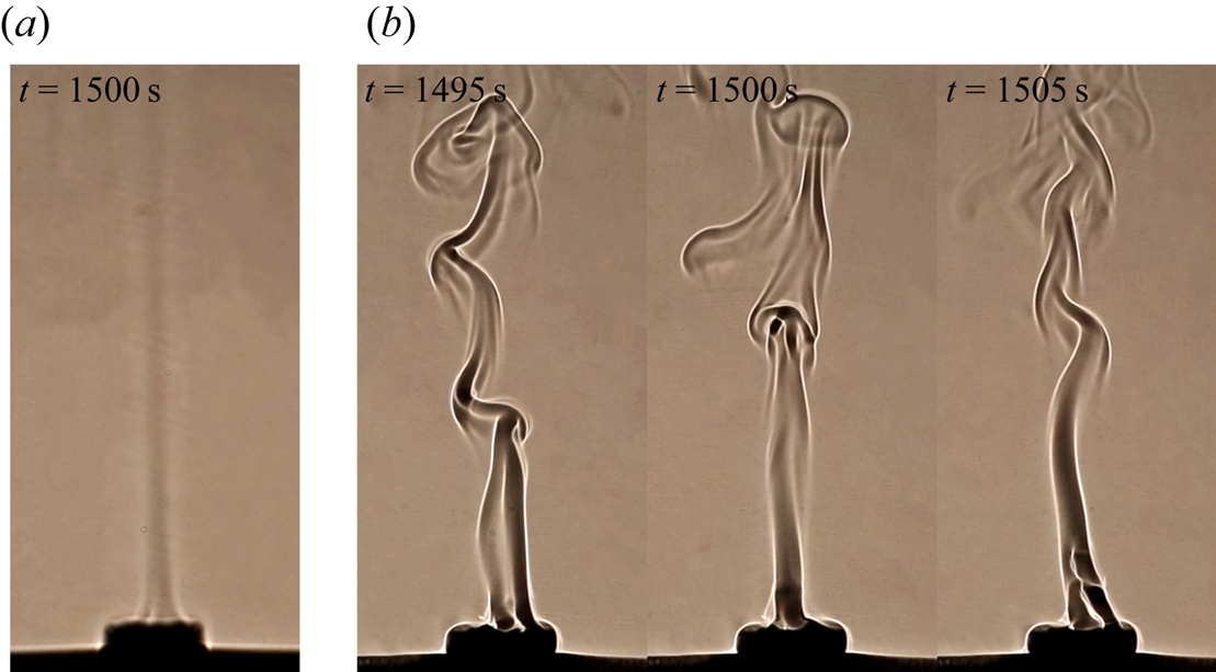
Figure 11. Flow structure of the plume in the fully developed stage for (a) Ra = 1.18 × 10⁵ and (b) Ra = 2.34 × 10⁶.
We also measured the velocity of the plume in the fully developed stage, which is shown in figure 12. In this study, the velocity was obtained only for the plume of the unsteady mode because the plume of the unsteady mode has many wrinkles in the shadowgraph image (see, e.g. figure 11b), which may be used to measure the velocity of the plume in the fully developed stage, but that of the steady mode does not (see, e.g. figure 11a). Figure 12 shows that there is a sound linear relationship between the experimental results and the scaling prediction, which is consistent with the scaling law of Wpsv ~ Ra 1/5 (also see figure 9b). Also, the function of the velocity in the fully developed stage may be expressed as
 \begin{equation}{W_{psv}} = 0.60R{a^{1/5}} - 5.99.\end{equation}
A large intercept (= −5.99) is present in (4.5), as also shown in figure 12. Further examination of the experimental results shows that such a large intercept is a result of the increase in the velocity in the fully developed stage compared to that in the equilibrating stage (see figure 9). That is, the velocity on the open cylinder in the fully developed stage is also influenced by the circulation in the water tank, which results in a difference, and thus a large intercept, from that proposed by the scaling analysis without consideration of the circulation in the water tank.

Figure 12. Velocity of the plume with puffing mode in the fully developed stage for different Rayleigh numbers.
4.2 Transition of the plume in the fully developed stage
A transition route is described by a steady, periodic, steady, periodic and chaotic plume in the fully developed stage, and was observed in the experiment. Figure 13 shows the typical flow structure of the plume in the transition route. The plume has a straight stem for Ra = 5.81 × 10⁵ and 1.41 × 10⁶, as shown in figure 13(a,c), in which the flow is steady. Additionally, the plume is flapping for Ra = 1.17 × 10⁶ in figure 13(b) but appears to puff at Ra = 1.77 × 10⁶ in figure 13(d). For Ra = 2.34 × 10⁶, the plume is chaotic, as shown in figure 13(e). The transition route to chaos is consistent with the previous numerical results of Zhang et al. (Reference Zhang, Qiao, Nie and Xu2021).

Figure 13. Transition of the plume in the fully developed stage. The red arrows indicate the flapping plume in panel (b) and puffing plume in panel (d).
4.2.1 Hopf bifurcation
The examination of the experimental results shows that the plume is steady for Ra = 5.81 × 10⁵ but periodic for Ra = 1.17 × 10⁶; thus, a Hopf bifurcation may occur between Ra = 5.81 × 10⁵ and Ra = 1.17 × 10⁶. Figure 14 shows shadowgraph images for Ra = 1.17 × 10⁶. The stem may curve locally, as indicated by the arrow in figure 14(a), and may develop downstream with time, as shown in figure 14(b–e). Such a plume was said to have a flapping mode by Zhang et al. (Reference Zhang, Qiao, Nie and Xu2021). Note that figure 14 shows the plume in only one quarter cycle.

Figure 14. Shadowgraph images of the plume with flapping mode in approximately one quarter cycle starting from t = 1328 s for Ra = 1.17 × 10⁶, where one cycle is Tc = 33.3 s.
To quantify the plume flapping, we measured the position of the plume stem from shadowgraph images. Figure 15(a) shows the x-coordinate of the stem (xp) at z = 150 mm for Ra = 1.17 × 10⁶. Here, xp is oscillatory with time and there are many weak oscillations induced by ambient perturbations. We also determined the power spectral density (PSD), which is shown in figure 15(b). The power spectral density shows that the flapping is periodic with the fundamental frequency ff = 0.03 Hz with a harmonic mode.

Figure 15. (a) Time series of the x-coordinate of the plume stem at z = 150 mm for Ra = 1.17 × 10⁶ and (b) power spectral density (PSD).
To describe the Hopf bifurcation in more detail, we measured the temperature in the fully developed stage. Figure 16 shows the time series of temperature at the point (0, 0, 7.5 mm). The time series of temperature remain steady for Ra = 5.81 × 10⁵ in figure 16(a) but periodic for Ra = 1.17 × 10⁶ in figure 16(b), which is consistent with the flow visualization in figure 14. Also, spectral analysis was conducted and is shown in figure 16(c). The plume is periodic with a fundamental frequency of ff = 0.03 Hz and harmonic modes for Ra = 1.17 × 10⁶. The fundamental frequency in this study is consistent with that in figure 15(b).

Figure 16. Temperature at the point (0, 0, 7.5 mm) for (a) Ra = 5.81 × 10⁵ and (b) Ra = 1.17 × 10⁶. (c) PSD of time series of temperature in panel (b).
4.2.2 Period bubbling bifurcation
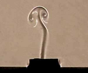
As indicated by Zhang et al. (Reference Zhang, Qiao, Nie and Xu2021), the plume on the open cylinder may become steady again with an increase in the Rayleigh number, which is referred to as a period bubbling bifurcation. Such an inverse bifurcation was also observed in the experiment for Ra = 1.41 × 10⁶. Figure 17 shows the flow structure and temperature of the steady plume for Ra = 1.41 × 10⁶. Thus, the plume stem is straight and the temperature is an approximately constant value, suggesting that the plume is steady. Bier & Bountis (Reference Bier and Bountis1984) indicated that for a nonlinear dynamical system with two or more governing parameters, period bubbling bifurcation may occur if the governing equation remains invariant after a symmetry transformation. In this study, there are three non-dimensional governing parameters (the Rayleigh number, the Prandtl number and the aspect ratio) that describe the convection system on the open cylinder, and the continuity, Navier–Stokes and energy equations under the symmetry transformation remain invariant. Thus, the convection system on the open cylinder satisfies the conditions of the period bubbling bifurcation (also see Bier & Bountis Reference Bier and Bountis1984 for details).

Figure 17. (a) Shadowgraph image of the plume for Ra = 1.41 × 10⁶ and (b) temperature at the point (0, 0, 7.5 mm) in panel (a).
4.2.3 Secondary Hopf bifurcation
With an increase in the Rayleigh number, a Hopf bifurcation from a steady to a periodic state occurs again. Figure 18 shows shadowgraph images of the plume for Ra = 1.77 × 10⁶. A puffing of the plume appears upstream on the cylinder, as shown in figure 18(a), and rises downstream with increasing time, as shown in figure 18(b–e). Finally, one new puffing of the plume appears upstream again on the cylinder in figure 18(f). Such a periodic plume has a puffing mode with a frequency of fp = 0.06 Hz. The examination of the experimental results indicates that the rising velocity of the puffing plume is constant and may be scaled with Wpsv ~ Ra 1/5 (see figure 12).

Figure 18. Shadowgraph images of the plume with puffing mode in one cycle starting from t = 1292 s for Ra = 1.77 × 10⁶, where one cycle is Tc = 16.7 s.
Figure 19 shows the time series of temperature and PSD for Ra = 1.77 × 10⁶. The temperature is oscillatory with a fundamental frequency of fp = 0.06 Hz and multiple harmonic modes, which is consistent with that in figure 18. Note that the amplitude of the fluctuations slightly reduces in a short time around t = 1481 s due to the presence of small perturbations in the experiment. The further examination of temperature time series and flow visualization shows that the small reduction of the amplitude has no influence on the flow regime but slightly decreases the harmonic of the fluctuations, as shown in figure 19(a).

Figure 19. (a) Temperature at the point (0, 0, 7.5 mm) for Ra = 1.77 × 10⁶. (b) PSD of time series of temperature in panel (a).
4.2.4 Transition to chaos
The plume becomes more complex with increasing Rayleigh number. The experimental results show that the flow structure of the plume may be irregular for larger Rayleigh numbers. Figure 20 shows the plume for Ra = 2.34 × 10⁶. In this study, the plume may be the puffing-type mode in figure 20(a–c) and the flapping-type mode in figure 20(d–f). Thus, the plume structure is the coexistence of the puffing and flapping modes, and the plume becomes chaotic for Ra = 2.34 × 10⁶.

Figure 20. Shadowgraph images of the plume starting from t = 1468 s with time interval of 2 s for Ra = 2.34 × 10⁶.
Figure 21 shows the time series of temperature and PSD for Ra = 2.34 × 10⁶. Clearly, the temperature time series are chaotic in figure 21(a), and PSD has only some bumps without any distinct peak frequency in figure 21(b). This means that the plume has become a chaotic state (see Hilborn Reference Hilborn2001 for the identification of the chaotic mode based on power spectral density). The further quantitative analysis of the chaotic plume will be presented in the following section. The numerical study by Zhang et al. (Reference Zhang, Qiao, Nie and Xu2021) indicates that the plume may undergo a period doubling bifurcation, a quasiperiodic bifurcation and finally a chaotic state in a very narrow range of Rayleigh numbers. Unfortunately, it is difficult to identify these bifurcations in such a narrow range of Rayleigh numbers with a variety of disturbances in the experiment.

Figure 21. Temperature at the point (0, 0, 7.5 mm) for Ra = 2.34 × 10⁶ (a). (b) PSD of time series of temperature in panel (a).
4.2.5 Entire route to chaos
Figure 22 shows a bifurcation diagram to characterize the entire route to chaos. Thus, the maximum and minimum non-dimensional temperatures in one fluctuation at the point (0, 0, 7.5 mm) were recorded for different Rayleigh numbers and are plotted in figure 22. Clearly, there is only one point for a steady plume and two points for a periodic plume, but there are many points for a chaotic plume in the bifurcation diagram. Note that only a few points are shown in figure 22 for a schematic of a chaotic state. The transition route to chaos may be described by a steady, periodic, steady, periodic and chaotic plume. Additionally, the range of the critical Rayleigh number is reported when a Hopf bifurcation (8.81 × 10⁵ < Ra < 1.06 × 10⁶), a period bubbling bifurcation (1.17 × 10⁶ < Ra < 1.30 × 10⁶), a secondary Hopf bifurcation (1.41 × 10⁶ < Ra < 1.61 × 10⁶) and a transition to chaos (2.06 × 10⁶ < Ra < 2.34 × 10⁶) occur.

Figure 22. A bifurcation diagram for the entire route to chaos with the Rayleigh number based on the non-dimensional temperature at the point (0, 0, 7.5 mm).
To characterize the transition route to chaos in more detail, the phase trajectories of the temperature time series at the point (0, 0, 7.5 mm) for different Rayleigh numbers are plotted in figure 23. Thus, we reconstructed the phase space of one-dimensional temperature time series T(t) using a time-delay reconstruction method (the embedding dimension m = 3 and the time delay τ), in which the new time series T(t + τ) and T(t + 2τ) were obtained (see Broomhead & King Reference Broomhead and King1986 for details of the phase space reconstruction). As shown in figure 23(a), the phase trajectory finally approaches a fixed point for Ra = 5.81 × 10⁵ in which the plume is steady. After the Hopf bifurcation, the plume becomes periodic for Ra = 1.17 × 10⁶, as shown in figure 23(b), in which the attractor is expressed as approximately a limit cycle. Thus, the phase trajectory is relatively concentrated in an annular region but not a good limit cycle due to the influence of the perturbations in the experimental environment. Also, the phase trajectory approaches a fixed point again for Ra = 1.41 × 10⁶ in figure 23(c), in which a period bubbling bifurcation occurs and the plume changes from a periodic to a steady state. Then, the secondary Hopf bifurcation occurs, and the attractor becomes approximately a limit cycle again for Ra = 1.77 × 10⁶, as shown in figure 23(d). For Ra = 2.34 × 10⁶, the phase trajectory becomes a strange attractor, as shown in figure 23(e), in which the plume is chaotic (see Ruelle & Takens Reference Ruelle and Takens1971 for strange attractor).

Figure 23. Phase trajectories of temperature time series at the point (0, 0, 7.5 mm) for (a) Ra = 5.81 × 10⁵, (b) Ra = 1.17 × 10⁶, (c) Ra = 1.41 × 10⁶, (d) Ra = 1.77 × 10⁶ and (e) Ra = 2.34 × 10⁶.
To quantify the characteristics of the attractor in the phase space, the fractal dimension was calculated (see Grassberger & Procaccia Reference Grassberger and Procaccia1983 for details). The fractal dimension is approximately 1.3 for Ra = 1.17 × 10⁶ and 1.2 for Ra = 1.77 × 10⁶, suggesting that the plume is periodic, but 2.2 for Ra = 2.34 × 10⁶, which means that the plume is chaotic. Thus, the results of the fractal dimension are consistent with the attractors in figure 23.
4.3 Heat and mass transfer
To validate the scaling law (3.11), the temperature gradient on the cylinder was calculated in the developed stage, and conversely, the Nusselt number (Nus) was obtained from the experimental results and is defined as
 \begin{equation}N{u_s} = \frac{{hD}}{k}\textrm{ = }{\left. {\frac{{\textrm{d}{T^ \ast }}}{{\textrm{d}{z^ \ast }}}} \right|_{wall}},\end{equation}
where h, k, T* and z* are the heat transfer coefficient, thermal conductivity, dimensionless temperature and dimensionless z-coordinate, respectively. Figure 24 shows the Nusselt numbers for different Rayleigh numbers. Clearly, the Nusselt number increases with increasing Rayleigh number, and a linear relationship exists between the experimental results and the scaling prediction by Nus ~ Ra 1/5. Also, the linear fitting function may be expressed as
 \begin{equation}N{u_s} = 0.45R{a^{1/5}} + 9.91.\end{equation}
Figure 24. Nusselt numbers for different Rayleigh numbers.
The Nusselt number in this study is smaller than that through the horizontal plate (also see Jiang et al. Reference Jiang, Nie and Xu2019). This is because the open cylinder may marginally reduce heat transfer due to the presence of the circulation in the cylinder in which the heated fluid is not easily convected away (also see Lewandowski et al. Reference Lewandowski, Bieszk and Cieslinski1992). Additionally, the Nusselt number for the smallest Rayleigh number is a little away from the fitting line in figure 24 because the scaling law of the Nusselt number can quantify the heat transfer under convective dominance but cannot quantify the heat transfer under conductive dominance (e.g. smaller Rayleigh numbers).
The flow rate of the plume in the equilibrating stage was also calculated using
 \begin{equation}{Q_s} = {\rm \pi}r_p^2{w_p},\end{equation}
where the radius and velocity of the plume were also measured from shadowgraph images, as described in figures 10 and 12. Figure 25 shows the flow rates for different Rayleigh numbers. A linear relationship is shown to be distinct between the scaling prediction by (3.12) and the experimental results. Also, the linear fitting function of the non-dimensional flow rate can be written as
 \begin{equation}Q_s^ \ast= 1.93R{a^{ - 1/5}} - 0.05.\end{equation}
Figure 25. Flow rates for different Rayleigh numbers.
The non-dimensional flow rate  $Q_s^\ast $ linearly decreases with Ra 1/5, as shown in figure 25. However, the dimensional flow rate Qs linearly increases with Ra 1/5, as shown in the scaling law (3.12) because the flow rate is normalized by ${\rm \pi}$κDRa 2/5.
5. Conclusions
In this study, a set of experiments was performed to investigate the thermal plume on an open cylinder after sudden heating. The shadowgraph technique was used for flow visualization and a thermistor was used for temperature measurement. Transient and fully developed plumes have been characterized for different Rayleigh numbers from Ra = 1.18 × 10⁵ to 2.34 × 10⁶. The dynamic evolution of the transient circular column plume on an open cylinder after sudden heating below has been scaled with the new scaling laws under different regimes. The transition route of the fully developed plume from a steady to a chaotic state has been presented.
The development of the plume undergoes a developing stage, an equilibrating stage and a fully developed stage after sudden heating. The shadowgraph image shows that the plume appears on the open cylinder in the developing stage and the flow structure varies for different Rayleigh numbers. Axial symmetry may be broken as the plume rises and the critical time for the break-up of the axial symmetry becomes small with increasing Rayleigh number. The velocity (or height) of the plume front has been scaled with the new scaling laws in the developing and equilibrating stages, which are validated by the experimental results. Additionally, the radius of the circular column plume was measured, which is also consistent with the scaling prediction.
The flow visualization indicates that the plume in the fully developed stage may undergo a succession of bifurcations. For small Rayleigh numbers (Ra ≤ 8.81 × 10⁵), the plume is steady. At higher Rayleigh numbers, a Hopf bifurcation occurs, where the plume becomes periodic with a flapping mode for Ra = 1.06 × 10⁶. Interestingly, the plume becomes steady again for Ra = 1.30 × 10⁶, which is referred to as the period bubbling bifurcation. Also, the plume becomes periodic again with a puffing mode for Ra = 1.61 × 10⁶ after a secondary Hopf bifurcation. If the Rayleigh number is sufficiently large (e.g., Ra = 2.34 × 10⁶), the plume may become chaotic. Additionally, based on temperature measurements, the spectral analysis, the bifurcation diagram, the phase trajectory and the fractal dimension are also used to characterize the transition to chaos. The heat and mass transfer of the thermal plume on the open cylinder have also been quantified. The Nusselt number and the flow rate may be scaled with Ra 1/5 and Ra −1/5, respectively.
Acknowledgements
The authors would like to thank the National Natural Science Foundation of China (No. 11972072) for financial support.
Declaration of interests
The authors report no conflict of interest.
Data availability statement
All data that support the findings in this study have been included within the article.


