


Impact Statement
This work examines the effects of drought on agricultural insurance loss.
1. Introduction
Climate change significantly adds to the challenges facing agriculture, such as ensuring food security and preserving the economic prosperity of a growing global population (Rosenzweig et al., Reference Rosenzweig, Iglesias, Yang, Epstein and Chivian2001; Schlenker & and Roberts, Reference Schlenker and Roberts2009; Manandhar et al., Reference Manandhar, Pandey, Kazama, Kazama, Shrestha, Babel and Pandey2014; Fan et al., Reference Fan, Pena and Perloff2016; Deschênes and Greenstone, Reference Deschênes and Greenstone2018). Of noted interest are the varied effects of climate on weather-related phenomena, such as drought, heat waves, floods, hurricanes, and extreme precipitation. Drought in particular affects a number of factors associated with cropping systems, including excessive temperatures, water availability, long-term soil moisture drawdown, and levels of evapotranspiration (Rosenzweig and Parry, Reference Rosenzweig and Parry1994; Lobell et al., Reference Lobell, Schlenker and Costa-Roberts2011).
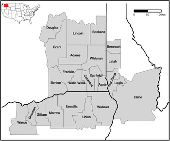
This analysis focuses on the highly productive inland Pacific Northwest (iPNW) agricultural region of the United States (U.S.) (Figure 1), which relies heavily upon dryland farming for cereal production (Karimi et al., Reference Karimi, Stöckle, Higgins, Nelson and Huggins2017; Yorgey and Kruger, Reference Yorgey and Kruger2017) and is considerably impacted by water availability. Our research objectives were to model how climatic effects for the iPNW are related to agricultural insurance loss, with a particular focus on drought-related claims for wheat. Two questions are addressed: What climate variables and temporal windows best relate to drought claims for wheat, and how do these relationships vary across the iPNW? Additionally, based on these optimum relationships, what climate variables have a greater influence on wheat insurance loss due to drought for the region, and can we utilize this framework for the prediction of insurance loss?
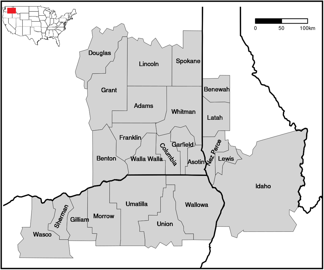
Figure 1. 24-county inland Pacific Northwest (iNPW) study area, which includes counties from Washington, Idaho, and Oregon.
From a regional perspective, the iPNW produces around 17% of the U.S. wheat harvest (Karimi et al., Reference Karimi, Stöckle, Higgins, Nelson and Huggins2017; Roesch-McNally, Reference Roesch-McNally2018). Given that cereal production is directly linked with variations in precipitation and temperature across much of the U.S. and the globe, iPNW wheat yields are significantly correlated with variability in plant available water during the growing season (Chi et al., Reference Chi, Waldo, Pressley, Russell, O’Keeffe, Pan, Huggins, Stöckle, Brooks and Lamb2017; Yorgey and Kruger, Reference Yorgey and Kruger2017). For example, 2015 iPNW wheat cropping outputs were negatively impacted by drought and extreme temperatures, evidenced in reduced crop yield outputs, increased agricultural insurance loss claim totals, and overall reduced wheat quality resulting in approximately $200 million of insurance loss in Washington state alone (Sandison, Reference Sandison2015; Seamon et al., Reference Seamon, Gessler, Abatzoglou, Mote and Lee2019). As one of the key agricultural production regions in the U.S., the iPNW supports a variety of cropping systems and management practices, which are dominated by dryland wheat farming (Chi et al., Reference Chi, Waldo, Pressley, Russell, O’Keeffe, Pan, Huggins, Stöckle, Brooks and Lamb2017). The region has cool-to-cold, wet winters and warm-to-hot, dry summers with considerable interannual variability based on regionalization across the Pacific Northwest (PNW) three state area (Abatzoglou et al., Reference Abatzoglou, Rupp and Mote2014; Yorgey and Kruger, Reference Yorgey and Kruger2017). Agricultural production for the area is typically limited by water rather than by growing season length (Stöckle et al., Reference Stöckle, Higgins, Nelson, Abatzoglou, Huggins, Pan, Karimi, Antle, Eigenbrode and Brooks2018), with annual precipitation increases from west to east, ranging from 200 mm to over 600 mm (Schillinger et al., Reference Schillinger, Papendick, Mccool, Zobeck and Schillinger2010; Chi et al., Reference Chi, Waldo, Pressley, Russell, O’Keeffe, Pan, Huggins, Stöckle, Brooks and Lamb2017). Interannual climate variability in the region can lead to considerable variation in available moisture, temperature, and evaporative demand.
In terms of mitigating long-term and seasonal variability with regard to climatic impacts, crop insurance is a key mechanism that is used to reduce such risk (Miranda and Glauber, Reference Miranda and Glauber1997; Seamon et al., Reference Seamon, Gessler, Abatzoglou, Mote and Lee2019). Of particular note are long-term climatic variability impacts on short-term extreme weather events, as well as shifts in seasonal/subseasonal weather outcomes that are exacerbated by a changing climate over an extended period of time (Backlund et al., Reference Backlund, Janetos and Schimel2008; USGCRP, 2017). In the PNW alone, from 2001 to 2015, over 35,000 insurance claims were filed, of which 20,600 were for wheat (Seamon et al., Reference Seamon, Gessler, Abatzoglou, Mote and Lee2019). For the iPNW in particular, drought and heat insurance claims for all commodities resulted in approximately $760 million in insurance losses from 2001 to 2015, which account for approximately 55% of all losses for this time period. Given this relationship between climate and agriculture, our research focus was to determine which climate variables and temporal windows best relate to drought claims for wheat, and what spatial variability exists with regard to this climate/agriculture association. Armed with this optimized information, we then developed a predictive model for estimating agricultural insurance loss based on climatic influences.
2. Data and Methods
Two datasets were used for this analysis. The first dataset was the U.S. Department of Agriculture (USDA) agricultural crop insurance claim archive from 2001 to 2015 (http://rma.usda.gov). When U.S. farmers experience economic losses for particular agricultural commodities, they typically file a crop insurance claim for that loss, as a part of the Federal Crop Insurance Corporation’s program, which underwrites agricultural insurance policies in conjunction with private insurance organizations. The filing of a crop insurance claim is the result of a complex set of decision-making processes, where farmers may incorporate multiple factors, spanning biophysical, climatic, economic, and socio-demographic disciplines. Over time, these insurance claim records are systematically provided to the USDA, who administers the program via the USDA Risk Management Agency (RMA) and makes these data available as a public archive. For the purposes of this analysis, individual agricultural insurance claims for wheat due to drought were aggregated at the county level. We only included claims during January to September given our focus on winter wheat phenological cycles, and hereafter focused on annual claims for each county. The second dataset used was daily gridded climate data at 1/24th degree (4 km) spatial resolution for the four climate variables most associated with water availability (maximum temperature, precipitation, potential evapotranspiration, and the Palmer drought severity index [PDSI]) from Abatzoglou (Reference Abatzoglou2013). Daily values were summarized by county and to a monthly time scale, with totals aggregated for precipitation and potential evapotranspiration, and average values for maximum temperature and PDSI.
In order to explore the associations of climate to insurance loss, we constructed a set of time lagged climate variable design matrices, to search for the optimal seasonal temporal relationship between a climate variable (i.e., maximum temperature, precipitation, evapotranspiration, and PDSI) and a county’s seasonal wheat insurance loss due to drought. We used this optimization approach to identify the most influential county-level time periods per season that were best correlated to wheat/drought insurance claims. Our initial step was to perform a general comparison of county-level wheat/drought-related claim acreage to water availability variables (precipitation and potential evapotranspiration), as well as aridity (precipitation/potential evapotranspiration), to examine general trends over time (2001–2015). The purpose of this initial analysis was to verify that expected patterns of wheat/drought insurance loss acreage versus water availability were seen (e.g., counties with relatively lower precipitation totals had overall increased wheat/drought insurance loss acreage). These annual, county-specific ratios were calculated by taking the total number of acres of wheat/drought insurance loss and dividing it by the total number of acres for all other wheat damage cause losses. As the ratio approaches 1, we identify county/year combinations where drought was the dominant factor in terms of total farmland acreage attributed to insurance loss. These analyses are provided as a part of our supplementary materials.
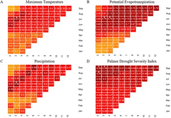
Second, we aggregated and associated climate data to wheat/drought crop loss seasonal totals by county, analyzing all outputs by using a time-lagged association by searching for the highest correlations between all combinations of monthly climate values (scaled and mean centered) and wheat insurance loss claims due to drought. We transformed annual loss amounts by a cube root function which resulted in a normal distribution of annual values. Following previous efforts to elucidate the optimum correlation (e.g., Du et al., Reference Du, Tian, Yu, Meng, Jancso, Udvardy and Huang2013), we examined these climate/insurance loss correlations for each county, based on each climate variable, using a 12 × 9 design matrix that considered different temporal periods (12 months for all climate data and 9 months for only winter wheat claims from January to September). Our goal was to evaluate which time-lagged windows were best correlated with overall wheat/drought insurance loss for a county, across the 2001 to 2015 time period (Figure 2). We then combined results of our county-specific time lagged correlation data across the 24-county study area, which resulted in an optimized county-level climate/insurance loss dataset (wheat claims due to drought), for each year, for the entire study area. This process created a new dataset of dependent and optimized independent (maximum temperature, precipitation, potential evapotranspiration, and PDSI) variables, which were used in the final step of our analysis: a regression-based random forest/decision tree analysis.
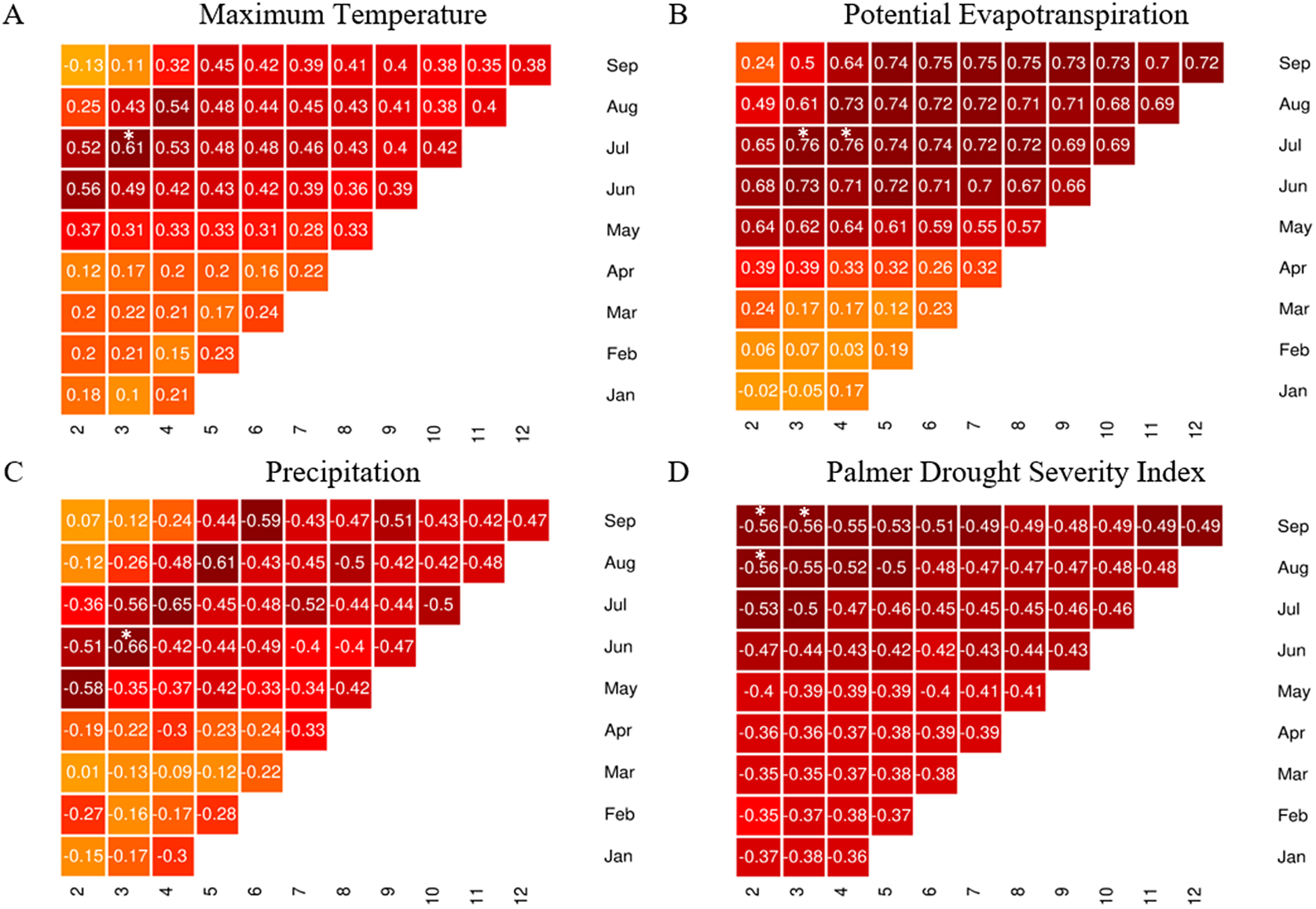
Figure 2. Correlation matrices for annual insurance loss due to drought and all four climatic variables: A) maximum temperature, B) potential evapotranspiration, C) precipitation, and D) the Palmer drought severity index for an example county (Whitman County, WA). The x-axis is the number of months of climate data aggregated and the y-axis is the last month of climate data. Each cell represents the correlation between climate data and a county’s annual insurance loss for wheat. For example, July 3 represents the correlation between annual loss and climate data for the months of May, June, and July. Though shown here for just one county, this calculation was performed for each county within the study area, across the 2001–2015 time period. Time windows that had the highest correlations (denoted above with an asterisk) for each county were used in subsequent random forest predictive modeling. A table with all county results can be found in the supplementary materials.
Regression decision trees are a method of constructing a set of decision rules on a predictor variable (Breiman et al., Reference Breiman, Friedman, Stone and Olshen1984; Verbyla, Reference Verbyla1987; Clark and Pregibon, Reference Clark, Pregibon and Chambers1992) that is continuous (versus categorical). These rules are constructed by recursively partitioning the data into successively smaller groups with binary splits based on a single predictor variable, with the goal of encapsulating the training data in the smallest possible tree (Prasad et al., Reference Prasad, Iverson and Liaw2006). Random forests, or ensemble decision trees, are a combination of many decision tree predictors, where each tree depends on the values of a random vector, sampled independently and with the same distribution for all trees in the forest (Breiman, Reference Breiman2001). Random forest modeling reduces the potential for overfitting through the use of bootstrap aggregation, averaging across many trees, and provides a level of feature importance for assessing predictor power. As a part of our random forest construction, we utilized 10-fold cross validation, a model validation technique used to assess the generalizability of the model. Model construction for this analysis utilized the recursive partitioning and regression trees package (rpart) within R (Atkinson and Therneau, Reference Atkinson and Therneau2000; Breiman et al., Reference Breiman, Friedman, Stone and Olshen1984).
3. Results
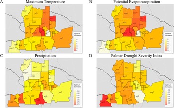
The results of our initial county-level wheat/drought acreage ratios (2001–2015), as compared to precipitation, potential evapotranspiration, and aridity are shown in the supplementary materials. Each observation represents the mean annual totals of each individual variable, for each county, from 2001 to 2015. We see expected climate/insurance loss relationships, with county-level precipitation totals, as well as aridity, inversely proportional to increased drought acreage ratios. Similarly, potential evapotranspiration totals increased as ratios increased. These general patterns supported moving forward to explore more specific spatiotemporal relationships of climate to insurance loss using our climate-lagged correlation framework. Using these time-lagged matrix correlation outputs, we mapped the spatial and temporal variations for each climatic variable, at a county scale (Figure 3).
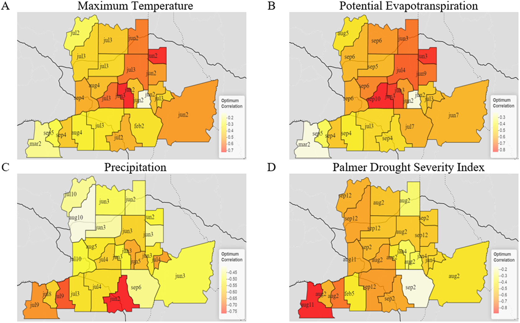
Figure 3. Spatial plot of correlation between insurance loss due to drought, for A) maximum temperature, B) potential evapotranspiration, C) precipitation and D) the Palmer drought severity index, across all counties within the study area, 2001–2015.
3.1. Potential evapotranspiration
An overview analysis of potential evapotranspiration (PET) from 2001 to 2015 for the study area indicates a climate gradient from east to west, with the annual maximum occurring in July. When examining optimum correlations of PET to cube root transformed wheat/drought insurance loss, the counties of Walla Walla, Columbia, and Whitman (Washington) had the highest values, along with Latah and Benewah counties (Idaho). Southernmost counties (Oregon) tended to have lower correlations than northern study area counties.
3.2. Precipitation
Regional cycles of precipitation, averaged for the period from 2001 to 2015, show increasing values from northwest to southeast. In all counties, the wettest months are November through January. Negative correlations of precipitation with insurance loss were highest in the southernmost study area counties, which tended to border the Snake and Columbia rivers (Wasco, Sherman, and Union counties, OR, and Columbia and Whitman counties, WA), ranging from −0.61 to −0.81. Counties further to the northwest (Franklin, Douglas, Lincoln, Spokane counties, WA) tended to have lower correlations, with April/May/June precipitation more highly correlated with drought loss for most counties.
3.3. Maximum temperature
Temperature tends to increase from southeast to northwest, which, as expected, is opposite to the pattern for precipitation. July was the peak month for high temperatures for every county in the iPNW. Maximum temperature was most highly correlated with drought in southeastern Washington counties, including Walla Walla, Whitman, Columbia, Garfield, and Spokane counties, WA, as well as Latah county, ID, ranging from 0.59 to 0.72. Temporally, most counties had an optimum relationship that fell between April and July, with Oregon counties and several western WA counties shifting that time window slightly later. The two counties with the highest correlations (Columbia and Garfield counties, WA), both had optimum time windows that included April.
3.4. Palmer drought severity index
PDSI spatial gradients had an increasing trend from southeast to northwest. PDSI optimum correlations with wheat/insurance loss appeared to have a spatial gradient that similarly increased to the northwest, with Douglas, Benton, and Grant counties, WA, as well as Wasco county, OR, having the highest correlation coefficients (r = 0.84). July/August/September was the most common window for optimum climate/insurance loss relationships, yet those counties with the highest correlations had window ranges that were much longer. As with precipitation, PDSI is negatively correlated with wheat/drought loss.
Overall results of our 24-county, 10-fold cross-validated random forest model using insurance dollar loss totals yielded a $ {R}^2 $
of 0.49 with a RMSE of approximately $30,880,545 (Figure 4). Individualized county model results provided variable performance, with
$ {R}^2 $
of 0.49 with a RMSE of approximately $30,880,545 (Figure 4). Individualized county model results provided variable performance, with $ {R}^2 $
ranging from 0.10 to 0.94 (see the Supplementary Material for individualized county model outputs). Feature importance rankings indicated that PDSI was the most influential predictor, with wheat prices and potential evapotranspiration as the second and third most important. Precipitation was the lowest predictor in terms of feature importance. When evaluating model error across training size (n = 348) using a learning curve analysis, we see considerable variation between training and validation error, which indicates that the model may be overfitting, and would potentially benefit from a reduction of complexity, or an increase in observations to improve performance.
$ {R}^2 $
ranging from 0.10 to 0.94 (see the Supplementary Material for individualized county model outputs). Feature importance rankings indicated that PDSI was the most influential predictor, with wheat prices and potential evapotranspiration as the second and third most important. Precipitation was the lowest predictor in terms of feature importance. When evaluating model error across training size (n = 348) using a learning curve analysis, we see considerable variation between training and validation error, which indicates that the model may be overfitting, and would potentially benefit from a reduction of complexity, or an increase in observations to improve performance.
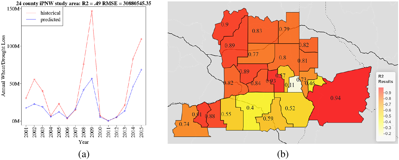
Figure 4. Historical versus predicted annual wheat insurance loss ($) due to drought, constructed using a random forest model, for the 24-county iPNW study area. Input variables were precipitation, maximum temperature, and potential evapotranspiration, as well as annual wheat pricing, from 2001 to 2015. Climate variables were refined using the aforementioned time-lagged correlation methodology ( $ {R}^2 $
= 0.49).
$ {R}^2 $
= 0.49).
4. Conclusions
The results of our climate lagged correlation analysis provide an interesting view of the spatial and temporal relationships of climate with localized insurance loss, with a particular focus on the region’s dryland wheat production. In particular, our results indicate the importance in understanding the varying temporal effects of drought-related climatic variables, as they vary spatially, which is also supported by the previous work of Semenov (Reference Semenov2009) and Lobell et al. (Reference Lobell, Hammer, Chenu, Zheng, Mclean and Chapman2015).
The results of our random forest model efforts indicate the potential importance of economic factors not accounted for in the current model, particularly given the underprediction of years with extreme drought claim totals. Given the considerable declines in wheat prices from 2008 to 2009 during the U.S. great recession (Fan et al., Reference Fan, Pena and Perloff2016), the underprediction of wheat insurance loss totals in 2009 may indicate the difficulty in the model to factor in economic considerations given the possible inflation of drought loss due to economics rather than climatic outcomes. By contrast, in 2015, which was a year of noted severe drought in the iPNW (Mote et al., Reference Mote, Rupp, Li, Sharp, Otto, Uhe, Xiao, Lettenmaier, Cullen and Allen2016), the model prediction was considerably closer to the observed loss. The comparisons of these two years may suggest a broader question around insurance loss and the interaction of climate and economics: are there economic thresholds that may produce climatic-associated loss claims, without clear justification in the climate data? While the developed model does attempt to broadly incorporate economic agricultural indicators (e.g., wheat pricing), the authors acknowledge that additional economic variables would potentially assist in addressing variance issues in loss prediction (consumer price indexing, unemployment rates, and housing/land values). Model performance may additionally be improved by using additional normalized climatic variables.
Given these associations of insurance loss with climate change, there are important considerations to contemplate. As future climatic conditions in the iPNW will likely lead to increased evapotranspiration rates, increased temperatures, and thus more extreme soil moisture deficits (Suyker and Verma, Reference Suyker and Verma2012), crop insurance programs will likely be negatively impacted. With limited long-term resilience, crop insurance efforts face added financial pressure under prolonged extreme weather conditions: subsidization mechanisms by the federal government to indemnify authorized crop insurance providers have typically only 1 year of coverage in cases of severe claim payouts (USDA RMA, 2016). As such, future extreme conditions for crop commodity systems, particularly around water availability, will likely increase the likelihood of financial stress with consecutive year drought events.
Author Contributions
Conceptualization: E.S., P.E.G., J.T.A.; Data curation: E.S.; Formal analysis: E.S.; Funding acquisition: P.W.M., P.E.G.; Investigation: E.S.; Methodology: E.S., P.E.G., J.T.A.; Project administration: E.S.; Resources: P.E.G., J.T.A.; Supervision: P.E.G., J.T.A., P.W.M., S.S.L.; Validation: E.S., J.T.A., S.S.L.; Visualization: E.S., J.T.A.; Writing—original draft: E.S.; Writing—review and editing: all authors.
Competing Interests
The authors declare no competing interests exist.
Data Availability Statement
A supplementary appendix as well as associated datasets can be found at https://doi.org/10.5061/dryad.h9w0vt4kh.
Ethics Statement
The research meets all ethical guidelines, including adherence to the legal requirements of the study country.
Funding Statement
This study was supported by a grant from the National Oceanic and Atmospheric Administration under grant number NA15OAR4310145, as well as by the National Institute of General Medical Sciences of the National Institutes of Health under award number P20GM104420. The content is solely the responsibility of the authors and does not necessarily represent the official views of the National Oceanic and Atmospheric Administration or the National Institutes of Health.
Provenance
This article is part of the Climate Informatics 2022 proceedings and was accepted in Environmental Data Science on the basis of the Climate Informatics peer review process.


 Open access