I.Introduction
A surge-type glacier oscillates between decade-long periods of quiescence and brief periods of surge motion (Reference Meier and PostMeier and Post, 1969). The dramatic and unusual behavior during surge motion is one of the most intriguing scientific problems in glacier dynamics. Although the quiescent phase of motion lacks the spectacular elements of the surge, it provides a unique opportunity for examining factors which control the normal motion characteristic of most glaciers. During the quiescent period, ice speed is much less than needed to maintain a steady state with climate. Year by year, one sees a progressing sequence of different geometrical states and motion characteristics, all in the same valley geometry. This sequence of natural experiments can define how changes in geometry of a glacier cause changes in its speed. The relationship between these changes is fundamental to the understanding of how glaciers adjust to climate change (Reference NyeNye, 1960).
In this paper we examine the natural sequence of experiments performed by Variegated Glacier in the period 1973–81. This interval includes the latter half of the quiescent phase of motion between the surges of 1964–65 Reference PostPost, 1969) and 1982–83 (Reference KambKamb and others, 1985). Variegated Glacier is a temperate glacier (Reference Bindschadler, Harrison, Raymond and CantetBindschadler and others, 1976) with a strong seasonal variation in speed (Reference Bindschadler, Raymond and HarrisonBindschadler and others, 1978). The geometry and speed of Variegated Glacier have been analyzed in substantial detail at two times: in 1973–74 (Reference Bindschadler, Harrison, Raymond and CrossonBindschadler and others, 1977) and in 1977–78 (Reference Kamb and EchelmeyerKamb and Echelmeyer, 1986). Observational results from the complete interval 1973–81 are available from World Data Center A — Glaciology in an annual series of unpublished data reports (Bindschadler and others, unpublished [a]–[d]; Raymond and others, unpublished [a]–[c])and a summary report (Raymond and others, unpublished [d]). This paper presents a full season-by-season history of changes in geometry and speed defined by these measurements, and attempts to relate the changes in terms of ice deformation and basal sliding. It also identifies the dynamic state of the glacier that existed at the time of the initiation of surge motion in 1982. A related paper (Reference Raymond and HarrisonRaymond and Harrison, 1987) examines the statistical fit of several motion models to the data presented here.
In addition to the seasonal variation in geometry and velocity reported and discussed in this paper, intensified measurements started in 1978 led to the discovery of short time‒scale variations in velocity and associated phenomena in the terminal stream discharging water from the glacier. These results have been reported elsewhere (Reference Harrison, Raymond and MacKeithHarrison and others, 1986;Reference Humphrey, Raymond and Harrison Humphrey and others, 1986; Reference Raymond and MaloneRaymond and Malone, 1986; Reference Kamb and EngelhardtKamb and Engelhardt, 1987). The dramatic surge motions of 1982 and 1983 have been described by Reference KambKamb and others (1985).
II. Changes in Geometry and Velocity
A. Measurements
The geometry of Variegated Glacier in June 1973 is displayed in Figure 1. Changes in thickness subsequent to June 1973 were measured by surveying surface markers spaced along the center line over most of the glacier length (Fig. 2). Repeated surveys of markers gave velocity averages over various time intervals (Fig. 3). This paper discusses primarily winter and summer seasonal intervals, as defined by the list of survey dates given in Table I. The extent of spatial coverage, spatial density of data points, and measurement time-scales is displayed, for the most part, by these figures and the table.
Less systematic measurements were made at other times, at off –center –line locations, across several transverse lines, and in the principal tributary (Fig. 1). These accessory data are available in the data report series (Bindschadler and others, unpublished [a]–[d]; Raymond and others, unpublished [a]‒[c]) and are not presented in detail here. We will however, have occasion to refer to them.
B. Treatment of the Data
Reference Center-Line and Datum Geometry
To establish distance along the glacier in a unique way, a reference center line (Fig. 1) was defined to follow closely the center-line markers established in June 1973. The kilometer distance cited in the text and figures refers to the distance from the glacier head along this line.
Datum geometries for the glacier and valley were established by assigning values of surface elevation, center-line bed elevation, cross-section area, surface width, and change of surface width with unit change in depth at each datum center-line point (Fig. 1). Surface-elevation values were based on elevations measured in June 1973 at M ¼ km intervals and on hand interpolation where reference points were not located precisely at survey points. Bed-elevation values were based on seismic reflection measurements, radio echo-soundings, and bore-hole depths as compiled from various sources by Kamb and Echelmeyer (1986, fig. 8) except between Km 0 and Km 3 where radio echo-soundings by MacQueen (unpublished) were used. Cross-section area, width, and its change with depth were measured in 1973 by seismic reflection at six transverse lines (Reference Bindschadler, Harrison, Raymond and CrossonBindschadler and others, 1977) and these were interpolated at intervening locations based on U.S.G.S. map Sheets. The longitudinal positions of the six transverse sections are labeled by capital letters in the figures displaying longitudinal profiles. Above Km 3, the surface and bed geometry are complex and are not necessarily well represented by center-line surface and bed elevations.

Fig. 1. Geometry in June 1973. (a) Map shows center line with Km ticks indicating distance from head, (b) Longitudinal profile gives the center-line elevations of the surface and the bed. Bed elevation measured by seismic reflection (Reference Bindschadler, Harrison, Raymond and CrossonBindschadler and others, 1977) is represented by dashed line. Subsequent radio echo-sounding (MacQueen, unpublished) and bore-hole depths (personal communication from W.B. Kamb) have provided improved depth estimates on the upper glacier. The current “best bed” is shown by the solid line, (c) Shows longitudinal variation in width, change of width with height, and shape factor.

Table I Data on seasonal variation time windows
Representation of Data as Longitudinal Profiles
Below Km 3, where data values were regularly spaced, a piece-wise continuous longitudinal profile was produced by optimal interpolation of measurements made within 50 m of the center line. Actual display of the profiles in plots is by straight-line segments joining points evaluated at integral ¼ km values of x. This is close to the spacing of the actual data values which, however, were not usually located precisely at integral ¼ km values of x. Above Km 3, where data points were not on a single longitudinal line and were irregularly spaced, data were interpolated by hand.
C. History of Change in the Main Valley
Elevation Changes
A progressive trend of annual elevation change from one September to the next occurred over most of the glacier length (Fig. 4). Between 1973 and 1981, there was a progressive thickening of the upper glacier from about Km 2 to Km 10 with a maximum of about 60 m between Km 6 and Km 8, a corresponding thinning of more than 50 m near the terminus below Km 18, and a steepening of the intervening stretch of the glacier. The boundary between net thickening and thinning relative to 1973 is well-determined after 1975 and moved from Km 9.8 to Km 11.6 between 1975 and 1981, which corresponds to a down-glacier migration at an average speed of 0.3 km a−1. The maximum elevation change appears as a bulge, which also showed evidence of a down-glacier propagation from 1974 to 1981 at a similar average speed.
The total elevation change after 1973 is unknown above Km 2, since measurements at fixed index locations were made only after 1976. However, from 1976 to 1981, elevation changes were smaller than the annual accumulation and unsystematic. Also, aerial photographs show that this zone was only mildly affected by the surges of 1964–65 and 1982–83. There is apparently no progressive evolution of this highest part of the glacier. This nearly steady-state condition may arise because this zone is separated from the main length of the glacier by a short complex ice fall between Km 2.0 and Km 2.7 (Fig. 1b).

Fig. 2. Elevation change relative to datum profile of June 1973. Note change in vertical scale for different years. Data points are from surveyed locations and elevations relative to the optimally interpolated datum profile. Dashed curve is fifth-order polynomial fit to the data points. Solid curve is an optimally interpolated fit to the data points. (Data points and digitized curves are tabulated in Raymond and others (unpublished [d]).)

Fig. 3. Horizontal velocity measured at the surface for various years (× — summer, late June or early July to early September; о — annual, September to September). Summer and annual velocity curves are determined from the corresponding data points using optimal interpolation. Winter uw curves are found from the annual uy and summer us curves by using the equation tyUy = ts.us + (ty ‒ ts)uw where ty and ts are the lengths of the annual and summer survey intervals. For annual and winter measurements, the year indicates the end of the measurement period. (Data points and digitized curves are tabulated in Raymond and others (unpublished [d]).)
Velocity Changes
There were prominent year-to-year changes in velocity which are displayed in Figure 5. The changes were largest in the upper part of the glacier between Km 3 and about Km 11, and there showed a progressive year-to-year increase in velocity. There also appears to be a bi-annual rhythm to the velocity increase. The smaller changes on the lower glacier showed some reversal of trend over time. Above Km 2, there was no progressive change in velocity. A strong seasonal variation in velocity existed over most of the glacier length as described earlier (Reference Bindschadler, Harrison, Raymond and CrossonBindschadler and others, 1977). The seasonal variation and year-to-year trends at selected fixed locations are illustrated in Figure 6. Before 1977, summer velocity increased faster than winter velocity, so that the amplitude of seasonal variation in velocity also increased. After 1978, summer and winter velocity increased in parallel and the amplitude of seasonal variation stopped increasing.
D. Changes in the Tributary
Changes in the one major tributary (Fig. 1) are not as well-documented as in the main valley. Based on up to six markers, a general description is possible. Elevation increased roughly 40 m from 1973 to 1978. This change was about the same as the elevation change in the main valley between Km 5 and Km 6.5 where the tributary enters (Fig. 4). From 1978 to 1981, there was no consistent trend in elevation change, which contrasts with the continuing progressive increase in the main valley (Fig. 4). Similarly, the speed increased from 1973 to 1978, but there was no consistent change from 1978 to 1981. There was also a distinct seasonal variation in speed similar to that observed in the main valley. In 1978 and 1979, the seasonal difference in velocity was about 0.3 m d−1 compared to a winter velocity of 0.5 m d−1. The history of the seasonal variation is not well known.
It appears that, by 1978, the tributary reached an approximate steady state in which the velocity had increased enough to drain the mass-balance input and stop the progressive build-up of ice mass there.
E. Prediction of Changes
Reference BindschadlerBindschadler (1982,unpublished) developed a numerical model to predict changes of Variegated Glacier between its surges. The model calculated changes in thickness with time from the longitudinal variation of ice flux and local width-averaged mass balance. Ice velocity and flux were calculated from ice deformation with no basal sliding. By fitting the model to the measured geometry and velocity in 1973 and driving it with the average mass-balance distribution observed from 1972 to 1976, he predicted changes in thickness and velocity in future years (Reference BindschadlerBindschadler, 1982, figs 12 and 14).

Fig. 4. Elevation change from September 1973 to following Septembers, based on the optimally interpolated elevation-change profiles of Figure 2. Above Km 2, elevation changes were small and unsystematic from 1976 to 1981 and are assumed to be small relative to 1973.
Over the length Km 5 to Km 16 that Bindschadler examined, the shape of the predicted longitudinal profiles of elevation change and velocity agree remarkably well with the observed changes. The advance with time of the boundary betwen thickening and thinning, the growth of the bulge peaking between Km 6 and Km 7, and the increase in velocity over the upper part of the glacier are all predicted well. (Compare Figure 4 to Reference BindschadlerBindschadler (1982, fig. 12) and Figure 5b to Reference BindschadlerBindschadler (1982, fig. 14).) However, the size of the changes in both velocity and elevation predicted over a time interval comparable to 1973–81 are much smaller than what actually occurred. Thus, there is a quantitative discrepancy that needs to be examined.
The most fundamental discrepancy is associated with the under-prediction of velocity changes.Reference Bindschadler Bindschadler (1982) estimated deformational flow velocity from basal shear stress and ice thickness with rheological and geometrical parameters calibrated from measurements in 1973. He used a simple longitudinal averaging scheme to account approximately for longitudinal stress gradients; although this scheme had imperfections that could have led to erroneous local variations in velocity (Reference Kamb and EchelmeyerKamb and Echelmeyer, 1986), it should have been adequate to represent the large-scale flow pattern correctly. For lack of a generally accepted sliding law, Bindschadler was forced to assume no sliding in his model, which could be the source of the discrepancy. Whatever the cause, the under-prediction of velocity changes from geometry changes represents a serious problem for any attempt to model ice flow. In the remainder of the paper we shall be concerned with this discrepancy in velocity identified by the model results. However, we shall discuss it by examining directly the relationship between observed velocity and observed geometry changes.
The failure of the model to predict accurate elevation changes arises in part from the under-prediction of velocity changes mentioned above. In addition, Bindschadler (1982, unpublished) noted that observed surface mass balance and changes in ice thickness over the interval from 1973 to 1976 appeared to be inconsistent with the ice redistribution by the flow velocities that were actually measured. Ice thickness increased more rapidly than could be explained, especially above Km 7. Our own analysis of subsequent years confirms this inconsistency. It may be associated with problems that inevitably arise in the pragmatic application of a one-dimensional continuity model to a specific three-dimensional system described by incomplete data. It is necessary to account for differences between center-line and width-averaged thickness changes and mass balance, for input from ice-clad valley walls and all tributaries, and for possible changes in depth-averaged density.Reference Bindschadler Bindschadler (1982, unpublished) discussed the limitations of the data in assessing the possible impact of these sources of error in mass-balance accounting. We shall not discusss these problems here, but instead will limit our attention to the broader dynamical question of how observed velocity is related to observed geometry.
III. Changes in Ice-Deformation Rate
A. Background
The total surface speed of a glacier ucomes from two sources expressed as
Here u d is a deformation contribution arising from internal shearing between the surface and bed and u b is a sliding contribution.
The deformational contribution u bis commonly estimated from
where h is the surface-normal ice thickness τb is the shear stress at the bed, and K = 2A/(n + 1) and n are parameters determined by the flow law of ice described as ![]() . Equation (2) arises from integration of shear strain-rate over depth, assuming that surface-parallel shear stress varies linearly with depth from 0 at the surface to τb at the bed and that it is the dominant contribution to effective stress and the corresponding effective viscosity in the non-linear flow law. (See Reference PatersonPaterson, 1981.)
. Equation (2) arises from integration of shear strain-rate over depth, assuming that surface-parallel shear stress varies linearly with depth from 0 at the surface to τb at the bed and that it is the dominant contribution to effective stress and the corresponding effective viscosity in the non-linear flow law. (See Reference PatersonPaterson, 1981.)

Fig. 5. Surface horizontal velocity in summer (a) and winter (b). Curves are from Figure 3 for locations below Km 3. Above Km 3, curves are based on hand interpolation of data values.
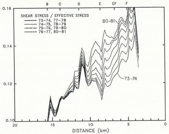
This section examines the effectiveness of Equation (2) to describe the relationship between changes in geometry and velocity observed on Variegated Glacier, and whether appropriate parameters K(or equivalently A) and n can be identified. To do this, we assume u b«u d so that u b∼u, and followReference Budd and Jenssen Budd and Jensen (1975) by comparing depth-averaged shear strain-rate u d/h with τb at different locations and times, which should define a line of slope non a log-log plot.
It would also be possible to express deformational velocity directly in terms of depth and surface slope without reference to basal shear stress using the assumptions above and additional assumptions that will be necessary to evaluate τb (e.g.Reference Kamb and Echelmeyer Kamb and Echelmeyer, 1986). This path would allow a direct comparison of velocity changes to changes in depth and surface slope. Echelmeyer (unpublished) has shown that a response factor is needed to account for changes in ice cross-section shape as an ice surface rises or falls in a fixed valley cross-profile. We avoid the need for explicit reference to the response factor by using Equation (2) and accounting for thickness, slope, and shape changes in the evaluation of τb as explained in section B below.

Fig. 6. Variation of surface horizontal velocity versus time at two longitudinal positions measured on a seasonal time-scale. Curves show the variation in velocity predicted from internal deformation with no sliding, using Equation (6) and the geometry and velocity for winter 1973–74 as a reference state with n = 3 (solid curve) and n = 4 (dashed curve where deviation from solid curve is perceptible). Differential speeds measured over short intervals in bore holes are represented by points (personal communication from H.F. Engelhardt and W.B. Kamb).
B. History of Base Stress
Shear Stress
The base shear stress beneath the center line is commonly estimated from the glacier geometry through the equation
where ρg = 0.088 bar m−1 is the weight per unit volume corresponding to ice density ρ (900 kg m−3), h is the local ice thickness normal to the upper surface at the center line, α is the surface slope, and f is a cross-section shape factor. Here, τsis referred to as the local slope stress. We calculate it using a slope averaged over 500 m; this corresponds to the resolution limit of our measurement spacing and is approximately 1–2 ice depths.
To account for longitudinal stress gradients, we used a longitudinal averaging based on the longitudinal coupling theory of Kamb and Echelmeyer (1986, Equation (3a)). It is expressed in terms of τsas

where lis a longitudinal coupling length that sets the effective length scale of the averaging. A constant value of l= 0.66 km (4l = 2.66 km) was used between Km 2 and 15. Above and below these limits, l= 0.25 km (4l = 1.00 km) was used because of lower ice depth. These coupling lengths are consistent with values found appropriate by Reference Kamb and EchelmeyerKamb and Echelmeyer (1986), who used their theory to analyze the distribution of velocity on Variegated Glacier during the years 1977–78. The base-stress distribution given by Equations (3a) and (3b) follows closely base stress estimated from Equation (3a) alone using a slope averaged over 2 km Reference Bindschadler, Harrison, Raymond and Crosson(Bindschadler and others, 1977), but it is somewhat smoother and, theoretically, more accurate.
Values of shape factor f were obtained from the numerical calculations tabulated by Reference NyeNye (1965, table IV), assuming a parabolic cross-section shape, width ratio determined from depth h and width w, and no basal slip. At cross-sections where section shape was known from seismic reflection measurements (B, C, D, E, EF, and F locations in longitudinal profile plots), f was also calculated from the actual shape (Reference Bindschadler, Harrison, Raymond and CrossonBindschadler and others, 1977, figs 3 and 7) using finite elements. The difference caused by deviation from parabolic shape was small (<6%) except at two sections near the tributary (EF ∼ 30%, F ∼ 11%).
The calculation of τb in the vicinity of the tributary between EF and F is, in any case, problematic, since the cross-section shape is not clearly defined at the confluence and the effect of the entering ice on the longitudinal force balance could be significant. Similarly, the surface and bed geometry above Km 3 are complex (MacQueen, unpublished) and Equations (3) are probably inadequate to capture the details of the distribution of τb there. In spite of these difficulties in estimating the full spatial distribution of τb we expect the broad features of the spatial pattern and the time trends to be correct.
The geometrical parameters α, h, w, and the resulting f all varied significantly with time and contributed to the shear-stress changes. Our interest is to compare velocity and stress. Therefore, the stress was computed from the average of the initial and final geometries of a survey interval, in order to approximate better the geometry responsible for the average velocity over that interval. The results for each winter interval are shown in Figure 7a.
Above Km 3, τb decreased with time, or the changes were small and unsystematic. Between Km 3 and Km 6, τb increased progressively from 1973 to 1979. From 1979 to 1982 the increase stopped, because increase in depth was compensated by decrease in surface slope. Between Km 6 and Km 13 there was a progressive increase over the complete interval. The largest changes occurred between Km 6 and Km 9, where both thickness and slope increased substantially with time (Fig. 4). Below about Km 13, τb decreased slightly or remained roughly constant where a decrease in depth was nearly compensated by an increase in surface slope.
Normal Stress
The basal normal stress σ b beneath the center line may be estimated from
Results for winter intervals are shown in Figure 7b. Corresponding effective normal-stress distributions are considered in section IV.B based on a theoretical calculation of water pressure.
C. Deformation of the Ice Column
Depth-averaged shear strain-rate is given by u d/h To estimate it, we assume zero sliding velocity (u b = 0), so that u d = u. The errors from this assumption should be smallest in winter, when u and presumably u b were at their seasonal minima. Therefore, we used the velocity measured in winter. Because the ice depth h is slowly varying over most of the glacier length (Fig. 1), the pattern of variation in shear strain-rate appears rather similar to the pattern for winter velocity (Fig. 5b). When estimated in this way, a maximum average shear strain-rate of 1.8 × 10⁻³ d−1 occurred in the vicinity of Km 4 during the winter of 1980–81.

Fig. 7. Evolution of center-line basal shear (a) and normal (b) stress estimated using Equations (3) and (4). and geometrical parameters described in the text.
For comparison, the pattern of longitudinal strain-rate (∂u/∂x) during the winter seasons can be inferred from Figure 5b. A maximum magnitude of longitudinal strain-rate of 0.15 ×10⁻³ d−1 occurred in the vicinity of Km 8 in the winter of 1980–81. At all locations and winter seasons, the longitudinal strain-rate was less than 0.2 times the depth-averaged shear strain-rate. Under these circumstances, softening of the ice column by coupling of the longitudinal strain-rate or corresponding deviatoric stress component into the effective non-linear ice viscosity should have a negligible effect on ud(Reference Raymond and ColbeckRaymond, 1980). Therefore, Equation (2) would not be expected to be invalid because of longitudinal strain effects.

Fig. 8. Depth-averaged shear strain-rate estimated as winter velocity (uw) divided by ice thickness (h) versus base shear stress (Fig. 7a). Points are computed for every ¼ km and every year 1973–81 for which data are available. Line represents prediction from flow law recommended by Reference PatersonPaterson (1981) for temperate ice (n = 3. A = 5.3 × 10⁻¹⁵ k Pa−3 s−1 = 0.167 bar−3 a−1). Curves join data points from fixed locations indicated by Km positions. Circles indicate data points from winter 1973–74; stars indicate dala points from winter 1980–81. Data points from intervening winters are not distinguished by distinct symbols in order to maintain clarity where density of data points is high.
These ideas are tested in Figure 8 by plotting u/hversus τb using values calculated every integral ¼ km for winters 1973–74 through 1980–81. The distribution predicted from Equation (2) using the flow law recommended by Paterson (1981; T = 0°C, A - 0.167 bar−n a−1, n = 3, K = 2.28 × 10⁻⁴ bar−3 d−1) is also shown for comparison. The overall pattern of data points is reasonably consistent with Paterson’s recommended parameters. Notice that most points from the winter 1973–74 lie below the expected distribution, while the data points from the winter 1980—81 lie above it. Additionally, points for which τb ≥ 1 bar suggest a slope steeper than n = 3.
The curves in Figure 8 link data from different years at selected fixed locations representative of the upper and lower parts of the glacier. Such curves, for all locations, cut across the spatially determined pattern of data points with slopes that are greater than correspond to n = 3. Steep slopes are especially noticeable on the lower part of the glacier at all locations below Km 10, where τb and u remained roughly constant and h decreased, thus giving increased u/hat constant τb and a nearly vertical trace on the plot (e.g. curve for Km 14 in Figure 8). On the upper part of the glacier at locations between about Km 3 and Km 7, there appears to be an increase in slope beginning in 1977 (e.g. curve for Km 5 in Figure 8). Figure 8 shows that changes in velocity over time at a fixed location were distinctly anomalous in comparison to the spatial pattern.
D. Velocity Anomaly
The parameter Kin Equation (2) can be calibrated from measured values of u, τb, and hat a reference time and location, so that

This presumes that u b = 0 for the reference measurement. The deformational velocity u d at any other time and/or location is then predicted to be

The difference between measured surface velocity u and u d predicted from Equation (6) defines a velocity anomaly u a
In the next section we assume that any such unexplained velocity arises from basal sliding; this is implied by Equation (1).
To apply Equations (5)–(1), we took the currently accepted value of n = 3 (Reference HookeHooke, 1981; Paterson 1981) and calculated K at each location from the values of u τb and h measured there over the winter 1973–74. This procedure assumes that u b = 0 at all locations in the winter 1973–74. The resulting values of K have a mean of 1.5 ×10⁻⁴ bar−3 d−1 and show a spatial variation up to about 30% from the mean with above-average values between Km 5 and Km 9, near average between Km 9 and Km 11, and below average below Km 11.
The mean of K is smaller than the value of K = 2.3 × 10⁻⁴ bar−3 d−1 predicted from Paterson’s preferred parameters. This difference is also evident in Figure 8 by comparing the data points for the winter 1973–74 with the line predicted from Paterson’s parameters. Thus, the glacier was apparently stiffer than what Paterson identified as typical temperate ice. Any actual sliding motion not taken into account by our no-slip assumption would make this difference even larger. That assumption, therefore, appears to be reasonable. In terms of the experimental flow law found byReference Duval Duval (1977), the mean value of K would be consistent with tertiary creep of temperate ice with a water content of about 0.1%.
The spatial variation of K corresponds to a deviation of data points for the winter 1973–74 from any single straight line of slope 3 in Figure 8. Such a spatial variation in apparent flow law is also evident in the analyses of the velocity in 1973–74 by Reference Bindschadler, Harrison, Raymond and CrossonBindschadler and others (1977, fig. 7), Reference BindschadlerBindschadler (1982, fig. 9), andReference Raymond and Harrison Raymond and Harrison (1987, fig. 2). It could arise from: (i) basal sliding, (ii) data errors in surface velocity, elevation, ice depth, and cross-section shape, (iii) inadequacy of Equations (2) and (3), or (iv) a real longitudinal variation in ice stiffness. We assume that (ii) is the dominant contribution and that the same errors influence Equations (2) and (3) in a similar way at all times so that the apparent value of K does not change with time.
The variation of u dwith time predicted from Equation (6) at two fixed locations is shown by curves on Figure 6. Figure 9 shows u a given by Equation (7) for the summer and winter seasons. These anomalies represent the part of the seasonal velocity history that is not explained by geometry changes figured by Equations (2) and (3), and calibrated by Equation (5) in the reference interval winter 1973–74. It is significant that by 1981 u a may be 50% or more of u at locations between Km 3 and Km 9. The implications are discussed in section IV. First we discuss how u a relates to two other analyses of velocity on Variegated Glacier.
E. Discussion of Deformation Calculations
The prediction of u d expressed by Equations (2)-(6) is essentially the same as used by Kamb and Echelmeyer (1986) to examine the distribution of velocity measured on Variegated Glacier over the interval July 1977-July 1978. Our approach differs from theirs primarily in the calibration of K by choice of the reference values of u, τb, h and in Equation (6). Our choice emphasizes the development of anomalous velocity with time relative to the winter 1973–74; any peculiarities of the spatial pattern in the winter 1973–74 are folded into the analysis as a spatially variable K. Reference Kamb and EchelmeyerKamb and Echelmeyer (1986) were concerned with the spatial pattern of velocity at only one time interval (1977–78) and calibrated K at a single reference location (Km 9.5). This gave a value of K = 2.4 × 10⁻⁴ bar−3 d−1 in good agreement with the Paterson value. With this spatially constant value of K, they predicted u d(x), which matched the measured u(x) very well over most of the glacier length; the only significant differences occurred up-glacier from Km 5, which they attributed to localized sliding at rates up to 0.2 m d−1 (Kamb and Echelmeyer, 1986, fig. 9).
Because of the differences in calibration of K, these two approaches are not directly comparable. Both predict anomalies localized on the upper part of the glacier. However, the spatial effect identified by Kamb and Echelmeyer was more narrowly confined and locally larger than the anomaly u a identified here (Fig. 9), which extended down to Km 8 and below. This difference arises primarily because the spatial pattern of velocity in the winter of 1973–74 contained similar features to that of 1977–78 (Fig. 5b), so that the spatial effect identified by Kamb and Echelmeyer was calibrated away by our spatially varying K.
It is also of interest to note that the value of K used by Kamb and Echelmeyer to fit the distribution of velocity in 1977–78 predicts a velocity in 1973–74 that is larger than measured everywhere between Km 3 and 15, which corresponds to a distinctly negative velocity anomaly over all of the well-measured length of the glacier. The negative anomaly is equivalent to the earlier recognition that in Figure 8 almost all of the data points from the winter 1973–74 lie below the line corresponding to the value of K given by Paterson’s preferred flow law, which is nearly equal to that used by Kamb and Echelmeyer. It is also related to the behavior illustrated in Figure 8 that velocity changes more rapidly at a given location than would be predicted from the spatial pattern. Such a negative anomaly could not reasonably be explained by basal sliding.
Like Kamb and Echelmeyer (1986),Reference Raymond and Harrison Raymond and Harrison (1987) examined the predictions of Equations (2)-(6) with spatially constant K. They showed that the mean value of K identified here and n = 3 produce the best least-squares fit of prediction to observations for the winter 1973–74 and that no time-independent, spatially constant value of K could match acceptably the full data set from all of the years, which is illustrated here by Figure 8.
This discussion underscores some of the ambiguity of predicting ice deformation and the importance of an accurate definition of the ice-flow law and a means to determine ice-structure parameters that affect it.
IV. Changes in Basal Sliding Velocity
A. Relationship of Velocity Anomaly to Basal Sliding
If Equation (6) gives a correct prediction of u d, then Equations (1) and (7) imply
where u b is the basal sliding velocity in the center of the glacier and u a is the deformational velocity anomaly defined by Equations (2), (3), (5), (6), and (7). Figure 9 would then display the longitudinal variation of center-line sliding velocity. The validity of Equation (8) is obviously subject to uncertainty from various sources.
The main uncertainty concerns the proper values of the flow-law parameters, which is evident in the discussion in section III.Е. In addition, ice stiffness could possibly change with time, in view of the effects of ice fabric and water content on the flow law (Reference DuvalDuval, 1977, 1981), and conceivable changes that could occur in the time-dependent flow environment of a surge cycle. We cannot entirely discount the possibility that softening of the ice contributed to the growing velocity anomaly u a between 1973 and 1981.
It is also clear that there is a limitation on the spatial resolution with which u b can be deduced. For example, if u b varies longitudinally, longitudinal stress gradients are set up which damp the resulting variation in u at the surface (Reference Balise and RaymondBalise and Raymond, 1985). The damping is large for velocity variations on a longitudinal scale of 10 ice thicknesses or less (3–4 km on Variegated Glacier), so that features at this scale are not likely to be captured realistically by the estimate of u bfrom Equations (6), (7), and (8). On Variegated Glacier, transverse velocity profiles (Reference Bindschadler, Harrison, Raymond and CrossonBindschadler and others, 1977) and the absence of cracking at the margins indicated sliding at the edges was negligible; therefore, if sliding occurred, it was more rapid in the center than at the edges. The resulting stress redistribution in comparison to the no-slip case causesf, τb, and u d to decrease beneath the center line (Raymond, 1980) and Equations (3), (6), (7), and (8) would underestimate u b there. Similarly, smaller-scale lateral variations in u b would be attenuated at the surface. Therefore, the estimated value of u b can at best represent a fairly large-scale spatial average over both length and width.
These various problems are not necessarily resolved by measurements of differential motion u d in bore holes. Such measurements were made by Kamb and Engelhardt over intervals of several weeks during the early parts of each of the summers 1978, 1979, and 1980 in the vicinity of Km 7 on Variegated Glacier. Preliminary analysis of the tilts (personal communication from H.F. Engelhardt) indicates values of u d plotted in Figure 6. A detailed analysis of measurement error has not been made but, based on the measurement interval of 3–4 weeks, an accuracy of approximately 0.05 m d−1 or better is likely.
These bore-hole measurements clearly show that during the actual intervals of measurement (early summer) a large fraction of u a is caused by sliding. On the other hand, the bore-hole measurements indicate a dramatic increase in u d between 1978 and 1979 that is inconsistent with Equation (6) and also appear to suggest that during the winters of 1978–79 and 1979–80 u a was not caused by sliding but rather by anomalous deformation. However, this interpretation is not straightforward. The holes made in different years were not at exactly the same locations and therefore may have sampled different local variations at the bed. The measurement intervals were short and included the occurrence of mini-surges (Reference KambKamb and Engelhardt, 1987) during which there could be substantial perturbation of the internal deformation pattern (Reference Balise and RaymondBalise and Raymond, 1985). Therefore, there is considerable uncertainty about how u d and the corresponding u b measured in these bore holes relate to the average over large areas of the bed and the long time intervals, which Equations (2)-(9) attempt to predict.

Fig. 9. Velocity anomaly computed with n = 3 from Equations (6) and (7) for the summer (a) and winter (b) seasons.
From this discussion and with recognition of the seasonal change in velocity (Figs 5 and 6), it is fairly certain that the distribution of u a determined for summer is correctly interpreted as being dominated by sliding. The interpretation of u a determined for winter intervals is not clear. Since the spatial patterns of u a in summer and winter have essentially the same profile shapes (with the exception of the summer 1981) and differ primarily in magnitude (Fig. 9), it is at least reasonable to assume u a truly represents sliding during winter as well.
Even though there are interpretational problems, it is nevertheless important to investigate whether the estimated distributions of u b.can be explained by proposed sliding laws (e.g.Reference Lliboutry Lliboutry, 1968, 1979;Reference Budd, Keage and Blundy Budd and others, 1979; Reference FowlerFowler, 1986) which predict u b in terms of basal shear stress and water pressure. Toward this goal we will focus primarily on the winter distributions, in recognition that during summer the sliding velocity and underlying physical controls are tied to melt cycles dominated by short time-scale transients Reference Harrison, Raymond and MacKeith(Harrison and others, 1986; Humphrey and others, 1986; Raymond and Malone, 1986; Kamb and Engelhardt, 1987), which are not completely documented by data or easily approachable theoretically.
B. Control of Sliding Variations
Basal Shear Stress
Figure 10a shows a scatter plot of estimated u b versus τb based on all center-line locations at ¼ km spacing and summer and winter intervals 1973–81 for which acceptable data are available. It appears that high u b is restricted to high τb. One also finds apparently low values of u b at high τb. This latter result arises in part from the assumption in section III.D, that assumes u b to be zero everywhere in the winter 1973–74, even though τb ranges up to nearly 1.6 bar. Clearly, Figure 10a does not reveal a unique relationship between u b and τb applicable to all times and locations.
Figure 10b presents winter data from Figure 10a on a log-log plot. To isolate the behavior at specific locations, curves join data points from Km 4, 5, 6, 7, 8, and 9. Data points from locations below Km 9 correspond to quite low u b (Fig. 9a), and relative accuracy is especially poor. Curves corresponding to these lower-glacier locations are in the lower left or off the diagram and, for simplicity, are not presented.
From the perspective of Figure 10b, the following very speculative interpretations can be drawn. The data between Km 7 and Km 9 are roughly consistent and crudely define a trend of increasing u b with increasing τb Although the data from Km 4, 5, and 6 collectively scatter about the extension of this trend to higher shear stress, the variations at any one location are definitely inconsistent with it. It appears that between Km 7 and Km 4, there is a spatial trend so that, going up-glacier, u b becomes smaller for a given τb but apparent sensitivity of u b to change in τb becomes larger.
Basal Water Pressure
Measurements of basal water pressure P w are available only from a few locations and short time intervals during summers (Kamb and others, 1985; Kamb and Engelhardt, 1987). In order to extend this information in space and time, it is necessary to calculate the pressure.
The change in patterns of short-period velocity fluctuations and the termination of the major surge pulses in early summer suggest that by the latter part of each melt season the water flow had melted out a tunnel along the base of the glacier through which water flowed to the terminus stream (Kamb and others, 1985;Reference Harrison, Raymond and MacKeith Harrison and others, 1986; Humphrey and others, 1986). We shall assume that such a tunnel persisted during most of the winter and controlled the water pressure over wide areas of the bed. During the winter, the discharge was about 1 m3s−1 at the terminus and transients in the flow should have been small. It is reasonable to estimate P w in the tunnel, assuming steady state (Reference Raymond, Harrison and SenearRöthlisberger, 1972;Reference Spring and HutterSpring and Hutter, 1981). We assume that the tunnel is fed by water released from storage in the glacier and the ground, flowing to the tunnel through a distributed system of basal passageways under small lateral pressure gradients. Therefore, the steady winter discharge was assumed to vary spatially along the glacier length in proportion to the ice area up-glacier. This includes a step change in discharge at the tributary entrance to account for water from the tributary basin.
To calculate the distribution of P w for each winter, the geometry (Figs 1 and 4) and overburden stress (Fig. 7b) were based on the average of the previous fall and following spring values. Ice flow-law parameters for tunnel-closure rate and tunnel-wall roughness were identical to those used by Reference Raymond, Harrison and SenearRöthlisberger (1972) to match pressure measurements on Gornergletscher. These particular flow-law parameters correspond to much softer ice properties than appropriate for shearing in the main body of a glacier as discusssed in section III. Whatever the cause of this inconsistency, for example, special conditions of stress or ice properties near the bed (Lliboutry, 1983), it promotes caution in applying the theory. Nevertheless, predictions from these tunnel-closure parameters do also appear to be consistent with the limited basal water-pressure measurements that are available from Variegated Glacier during June and July of 1978, 1979, and 1980 at locations near Km 7 (Kamb and Engelhardt, 1987). Water levels measured in the later part of July that most likely reflected the pressure in a basal tunnel and tunnel pressures predicted using the mean summer discharge at the terminus of about 16m3 s−1 found by Humphrey and others (1986) both correspond to 14–15 bar below ice overburden. We assume the same tunnel parameters are also reasonable for winter.
Results for water pressure P w in the form of effective normal stress (σ b – P w) are shown in Figure 11. There is a one-to-one correlation between the maxima and minima in the spatial patterns displayed in Figure 11 when compared to the distribution of ((σ b – P w) calculated byReference Bindschadler Bindschadler (1983, fig. 1) for Variegated Glacier in 1973 using assumptions similar to ours. Our results give somewhat lower mean levels of (σ b – P w), primarily because of a difference in assumed ice flow-law parameters. We shall focus on the relative changes in space and time that are insensitive to this assumption and are controlled by surface-slope and ice-thickness profiles. Figure 11 shows that above Km 14 variations in space and time of (σ b – P w) were less than 10% of the mean. This can be compared with the fractional changes in shear stress, which were up to about 50% (Fig. 7a). From this, one might expect the sliding variations to be controlled by τb and displayed by Figure 10. Nevertheless, the variations in (σ b – P w) may be significant, especially if u bis very sensitive to (σ b – P w).
The small time-dependence of (σ b – P w) showed a gradual increase at locations down-glacier from Km 6 and a decrease at locations at Km 6 and above (Fig. 11). This boundary occurred at the peak in elevation change (Fig. 4). Down-glacier from the peak, the surface slope increased with time. Theoretically, as time passsed, the water discharge was driven out of the glacier with a higher head gradient, greater energy loss and conduit-melting rate, and a correspondingly faster creep-closure rate, which allowed a larger pressure difference between the flowing water and the ice. Above the peak in thickness change, the surface slope decreased with time and caused opposite effects. This direct relationship between surface slope and effective normal stress changes is a qualitative feature that we might expect to find for any model of basal water flow in which water pressure opposes closure of water-flow passageways. For example, it is predicted for water flow through linked cavities by Kamb (1987). These temporal trends in (σ b – P w) may Partially explain the difference in apparent sensitivity of u b to change in τb above and below Km 6 (Fig. 10b). Below Km 6, the effect on σ b by the increase in τb was opposed by increasing (σ b – P w). Above Km 6, the effect on u b by increase in τb was augumented by a decrease in (σ b – P w).
Above Km 10 there was a gradual, although not monotonie, increase in (σ b – P w) with distance up-glacier. This trend is related to the up-glacier increase in surface slope (Fig. 1) and is explained qualitatively by the same reasoning as in the foregoing paragraph. Again, we may expect this qualitative pattern to be consistent with other models of basal water flow. This spatial trend may be a partial explanation of the lower u b for given τb at the up-glacier locations.
These qualitative patterns in space and time indicate an inverse relationship between u b and (σ b – P w).
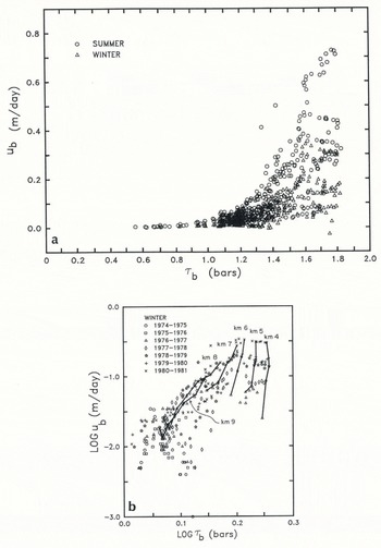
Fig. 10. a. Basal sliding velocity versus basal shear stress estimated at 0.25 km intervals on center line for summer and winter seasons 1973—81 (based on Figures 7a and 9).
b. Basal sliding velocity vesus basal shear stress for winter seasons 1973–81 (based on Figures 7a and 9). Curves link data points with same location.
Discussion of Sliding Behavior
Raymond and Harrison (1987) have used the data presented here in a search for a quantitative sliding law u b = f(τ b, σ b − P w) based on least-squares fit assuming several sets of possible flow-law parameters K and n. All of these choices yielded sliding laws such that u b increased with τb and decreased with (σ b – P w), thus indicating that our qualitative conclusions appear to be robust and insensitive to details of assumptions about K and nHowever, none of the best-fit sliding laws were good fits to the data in the sense of significantly reducing the residuals in the overall data set below the level achieved by ice deformation alone with an intermediate ice stiffness, for example, Paterson’s preferred value for temperate ice. Said another way, if predicted sliding u b were subtracted from measured surface velocity uto find corrected u d in Figure 8, the scatter would remain essentially the same.
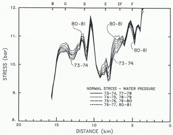
Fig. 11. Effective normal stress computed using steady-state flow of water in a “Röthlisberger” tunnel, geometrical parameters in Figure 1, stress from Figure 8b, and water flux at the terminus of 1 m3 s−1. Flow-law parameters (B and n in ε = (τ/B)n) and conduit Manning’s roughness (nʹ) were taken as B = 317 bar s1/3, n = 3. Nʹ = 0.1 m−1/3 s. The value of B corresponds to A = 3 × 10⁻¹⁴ K Pa−3s−1 = 1 bar−3 a−1 in the flow law έ = Aτn.
It is possible that the relationship we seek is obscured by errors in the data and theory used to derive u b, τb, and (σ b – P w). Certainly, we must suspect the calculation of basal water pressure. Perhaps the assumed basal tunnel did not exist over the full glacier length or the complete winter intervals (Humphrey and others, 1986) or the pressure on the adjacent bed was not tied to the pressure in the tunnel. If so, other water-flow models would be needed to calculate transport through linked cavities (Kamb, 1987), basal debris (Reference ClarkeClarke, 1987), or a combination that accounts for erosion and deposition of debris in the passageways. On the other hand, we expect the relationship between sliding rate and base stress to be affected by bed roughness or debris distribution, which could vary from place to place and with time. Whether the problem is caused by failure of the tunnel theory or non-existence of a spatially independent sliding law u b = f(τ b, σ b − P w), the resolution will apparently require knowledge of parameters related to detailed features of the bed structure. If this is true, it is effectively impossible to predict sliding rate without some calibration of the effects of the unknown bed structure.
C. Relationship to Surge Initiation
Despite the lack of success in discovering a “sliding law” that holds at all locations and times, the qualitative features are interesting. Of particular interest is the extreme sensitivity of u b to small changes in profile above Km 6 in the few years before 1982. Such sensitivity is similar to a failure behavior that may have been related to the eventual surge initiation in 1982.
The theoretical ratio I = τ b/(σ b − P w) is plotted in Figure 12.Reference Bindschadler Bindschadler (1983) referred to this ratio as the separation index, because as it rises, the probability of growth of basal cavities on the down-glacier sides of rigid bedrock bumps increases (Lliboutry, 1968; Kamb, 1970; Iken, 1981). More generally, we may expect that rising I increases the potential for rapid sliding independent of the actual basal structure. In view of the uncertainty in calculating basal water pressure and the corresponding effective normal stress, it is probably not realistic to ascribe much meaning to the actual numerical values of I in Figure 12. The spatial pattern, however, may be realistic. With this in mind, sliding rate appears to increase rapidly when I rises above a threshold that was reached in the few years before the surge between Km 4 and Km 7 (Figs 9b and 12). This location corresponds to the up-glacier flank of the growing topographic bulge centered between Km 6 and Km 7. Although the increase in τb (Fig. 7a) contributed strongly to the progressive rise in I, the drop in (σ b – P w). (Fig. 11) was the dominant influence just before the surge. This is of interest with regard to the location of the first rapid surge motion, which was predominant near Km 4. The surge initiation is discussed in more detail in a separate paper in preparation.
V. Summary and Conclusions
The velocity changes of Variegated Glacier from 1973 to 1981 during its normal phase of flow are not consistent with motion solely by ice deformation controlled by a flow law typical of temperate glacier ice identified by Paterson (1981, table 3.8). Nevertheless, if the data in Figure 8 are used to determine flow-law parameters, the scatter is much less than is apparent when velocity and bore-hole measurements from different glaciers are compared (e.g. Paterson, 1981, fig. 3.5). Therefore, these results promote some optimism for useful predictive modelling of ice deformation. However, it is clear from Figure 8 that at a detailed level, a time-and-space independent flow law without sliding cannot explain the time-and-space variations of the velocity. Comparison of Figures 5b and 9b shows that the theoretical changes in deformation flow based on a time-independent flow law with n = 3 predict less than half of the actual changes; in other words, most of the change in motion appears to be anomalous. Either the ice softened substantially with time or sliding became important. Accurate flow modelling will have to account for these potentialities.

If the cause of the anomalous velocity changes was basal sliding, any of the existing theories of sliding that relate sliding to basal stress and water pressure together with the theory of water pressure in basal tunnels are not adequate to predict the changes in a usefully quantitative way. Some of the qualitative characteristics of the observations are consistent with expectations from sliding theories. The quantitative discrepancy may arise from other relevant variables, perhaps associated with structure of the basal zone of the glacier.
The zone where anomalous velocity was largest and the 1982–83 surge eventually started lay on the up-glacier side of a topographic bulge that grew progressively from 1973 to 1982 in the upper part of the glacier. In this zone the basal shear stress increased with time except in the few years before 1982 when increased thickness was compensated by decreases in surface slope. The most important changes in this zone during this time interval may have been a decrease in effective normal stress caused by decreasing surface slope driving water flow down-glacier through this zone.
Acknowledgements
This research was made possible through research grants to the Universities of Alaska and Washington from the U.S. National Science Foundation (grant numbers EAR 7622463, EAR 7622500, EAR 7919424, and EAR 7919530). It was carried out with the permission of the U.S. National Forest Service (Tongas National Forest) and the U.S. National Park Service (Wrangell St. Elias National Park). Gulf Air Taxi, Yakutat, Alaska and Livingston Helicopters, Juneau, Alaska, provided logistical support. Many individuals contributed to the field program with dedication in both good and arduous times. We wish to mention especially colleagues at California Institute of Technology and the Project Office in Glaciology at the U.S. Geological Survey. R. Bindschadler and E. Senear carried out much of the data analysis. The final version of the paper incorporated valuable comments from K. Echelmeyer and two anonymous reviewers.