


Introduction
Unequal political participation in terms of education, income, age, and sex has commonly been studied in previous research. Unfortunately, another predictor of voting participation, partnership, has been overlooked in research on unequal turnout. Including mating structures and partnership formation in studies of unequal turnout, we can improve our understanding of who participates in politics. Marriage and cohabitationFootnote 1 have for a long time been understood as the most important source of interpersonal influence affecting the decision to turn out to vote or not (Wolfinger and Rosenstone, Reference Wolfinger and Rosenstone1980), and more recently, scholars have highlighted that partners tend to vote together (Fieldhouse and Cutts, Reference Fieldhouse and Cutts2012; Bhatti et al., Reference Bhatti, Fieldhouse and Hansen2018). Yet, previous research has overlooked that the patterns for how relationships are formed can have consequences for who participates in politics.
Recent experimental evidence supports a social mechanism of voter mobilization (Nickerson, Reference Nickerson2008; Gerber et al., Reference Gerber, Green and Larimer2008). Theoretically, these social aspects of political behavior may have important consequences for aggregate turnout. If voting is contagious, then the aggregate levels of turnout ought to be self-reinforcing, in the sense that, in a context where most people vote, you are likely to meet individuals who vote, and thus, social mobilization is common. However, in a context where turnout is low, most people you meet may not vote, and thus, social mobilization is less common. In other words, if turnout is high, it is likely to stay high; if turnout is low, it is likely to stay low (Fowler, Reference Fowler and Zuckerman2005).
This paper studies two questions. First, to what extent does assortative mating on the one hand, and social influence on the other hand account for correspondence in turnout behavior of couples? Second, does the combination of assortative mating and social influence contribute to social inequalities in turnout? The first question is present in the previous literature, in terms of the effect of entering a relationship (Stoker and Jennings, Reference Stoker and Jennings1995; Bhatti et al., Reference Bhatti, Fieldhouse and Hansen2018) and the effect of divorce or death of a spouse (Kern, Reference Kern2010; Hobbs et al., Reference Hobbs, Christakis and Fowler2014; Bhatti et al., Reference Bhatti, Fieldhouse and Hansen2018) on turnout. The previous studies have successfully established, what is sometimes called a companion effect, that voting together with one’s partner is common. This aspect of turnout behavior is also discussed in previous research on the question of selection vs social influence (Kandel, Reference Kandel1978; Huckfeldt and Sprague, Reference Huckfeldt and Sprague1987; Jennings and Stoker, Reference Jennings, Stoker and Zuckerman2005; Alford et al., Reference Alford, Hatemi, Hibbing, Martin and Eaves2011), but rarely quantified (for en exception see Kandel, Reference Kandel1978). Previous research has, however, paid less attention to the potential consequences of such findings.
This paper contributes to the previous literature in two ways. First, it contributes by providing a theoretical framework of how assortative mating can reproduce unequal voting participation. Second, it provides empirical analysis of the selection into marriage/partnership and the social influence within such relationships, using data from the British Household Panel Survey (BHPS) in and the UK Household Longitudinal Study (UKHLS).Footnote 2 I show that individuals who enter a relationship with an eventual voter increase their likelihood to vote, while individuals who enter a relationship with an eventual nonvoter decrease their likelihood to vote.Footnote 3 There are substantial differences between the groups also before entering the relationship. Thus, the results show that both mate selection and social influence explain correspondence in turnout behavior of couples. In addition, drawing on theories about partnership formation and mating patterns, I study the selection into the relationships. The main argument is that if the likelihood of entering a relationship with an eventual voter is unevenly distributed between socioeconomic groups, then self-reinforcing levels of turnout may be the case within socioeconomic groups. I show that, regardless of one’s own previous voting participation, the probability of entering a relationship with a potential voter is substantially higher among highly educated, high-income individuals than among less educated, low-income individuals. Moreover, I provide suggestive evidence that the behavioral changes when a nonvoter enters a relationship with a voter is larger among the more well-off citizens. The results indicate that mating structures may support a self-reinforcing element of socioeconomic inequalities in turnout.
Living together and the social aspects of turnout
For a long time, interpersonal mobilization has been seen as one of the key aspects in explaining voting participation (Campbell et al., Reference Campbell, Converse, Miller and Stokes1960; Lazarsfeld et al., Reference Lazarsfeld, Berelson and Gaudet1965). The same can be said for the findings that married individuals are more likely to vote than never married, divorced, or widowed individuals (Wolfinger and Rosenstone, Reference Wolfinger and Rosenstone1980). The theories highlighting interpersonal influence, for example, between spouses, are supported by correlations between marriage and turnout in the United States (Verba and Nie, Reference Verba and Nie1972; Wolfinger and Rosenstone, Reference Wolfinger and Rosenstone1980; Leighley and Nagler, Reference Leighley and Nagler2013) and in Britain (Denver, Reference Denver2008; Kern, Reference Kern2010). In addition, having a partner who votes is important for one’s own likelihood of turning out to vote (Stoker and Jennings, Reference Stoker and Jennings1995; Bhatti et al., Reference Bhatti, Fieldhouse and Hansen2018). Moreover, young people in Denmark who live with their parents are more likely to vote than young people who live alone (Bhatti and Hansen, Reference Bhatti and Hansen2012).
Recently, there has been a shift toward a more causal approach to testing the theoretical claims. For example, the death of a spouse has a larger negative impact on turnout if the spouse one lost was a voter (Hobbs et al., Reference Hobbs, Christakis and Fowler2014), and active mobilization in Get-Out-The-Vote (GOTV) experiments directed toward one person in a household has spillover effects to other members in the household (Nickerson, Reference Nickerson2008; Sinclair et al., Reference Sinclair, McConnell and Green2012). Moreover, support for contagion effects within households has not been limited to the United States but is also found in a European context, for example, by Bhatti et al. (Reference Bhatti, Dahlgaard, Hansen and Hansen2017) in a study using text messages to mobilize voters in Denmark. In sum, these recent studies support what is sometimes labeled a companion effect (Fieldhouse and Cutts, Reference Fieldhouse and Cutts2012), a causal story of a social voter.
Theoretically, the social aspects of turnout are influenced by and influence the aggregate turnout level. A study by Fowler (Reference Fowler and Zuckerman2005) shows that one person’s decision to vote on average affect four people in their decision to vote. The closer to the person who makes the first decision to vote one is the more likely to be influenced. One implication of this finding is that the average level of turnout is not easily changed. The larger the share of voters in the population, the larger the chance to be influenced positively by other people who vote Fowler (Reference Fowler and Zuckerman2005). The spillover effects within households can be seen as support for a self-reinforcing element in aggregate levels of turnout (Nickerson, Reference Nickerson2008). In other words, previous research provides theories of a social voter and compelling evidence of contagion effects between individuals within a household. The argument put forward by Fowler (Reference Fowler and Zuckerman2005) implies that the likelihood of such spillover effects is dependent on the aggregate turnout levels.
In sum, previous research suggests that there is a causal effect of having a voter in one’s household on one’s own turnout and that the occurrence of such contamination is more or less widespread depending on the aggregate turnout. What is not clear, though, is whether these self-reinforcing patterns are prevalent to the same extent in all groups in society.
Unequal voting participation
In a large body of literature, which focuses on the United States, it is well-established that more educated, higher-income individuals turn out to vote to a larger extent than do less educated, lower-income citizens (Verba and Nie, Reference Verba and Nie1972; Wolfinger and Rosenstone, Reference Wolfinger and Rosenstone1980; Verba et al., Reference Verba, Schlozman and Brady1995; Leighley and Nagler, Reference Leighley and Nagler2013). There is also a positive relationship between socioeconomic indicators and turnout in Western Europe, but the relationship is less pronounced than in the United States (Blais, Reference Blais2000). Regarding turnout in Britain, studies find that there is a weak positive relationship between education and voting participation (Denny and Doyle, Reference Denny and Doyle2008) or that there is no such relationship at all (Milligan et al., Reference Milligan, Moretti and Oreopoulos2004). However, a recent study finds that the class-based inequalities in turnout in Britain may be on the rise (Heath, Reference Heath2018). Moreover, a meta-analysis by Smets and Van Ham (Reference Smets and Van Ham2013) show that high income and education levels predict turnout in most of the studies in which income or education has been taken into account.
Although the literature on voting participation consistently demonstrates that some socioeconomic groups are more likely to vote than others, there is no consensus on why those relationships exist. For example, one explanation commonly put forward is that education reduces the cognitive costs and income reduces the economic costs of participation (Verba et al., Reference Verba, Schlozman and Brady1995). However, this causal story of education leading to increased voting participation has been challenged. Nie et al., (Reference Nie, Junn and Stehlik-Barry1996) argue that education ought to be seen as a sorting mechanism that determines one’s social network position. In other words, education can be seen as a relative rather than absolute value. Another perspective goes even further saying education is merely a proxy for preadult factors that can explain voter turnout and educational choice (Kam and Palmer, Reference Kam and Palmer2008). Theoretically, arguments from the recent debate on education and participation travel well to the relationship between income and voting participation. Income, similar to education, may be related to turnout in the following ways: Lowering the cost, determining one’s relative socioeconomic status, and/or being a proxy for preadult factors.
Combining the literatures of education and turnout and marriage and turnout, previous research finds a positive relationship between the education level of one’s spouse or partner and one’s own voting participation (Knack, Reference Knack1992; Stadelmann-Steffen and Koller, Reference Stadelmann-Steffen and Koller2014; Frödin Gruneau, Reference Frödin Gruneau2018). Moreover, Rolfe (Reference Rolfe2012) finds that having highly educated friends is a better predictor of voting participation than the individual’s own education level. These studies suggest that the relationship between education and turnout is not limited to the individual. Thus, the two revisionist stories of education as a sorting mechanism and education as a proxy are plausible explanations for such a correlation. However, what is not clear from these studies is whether the positive relationship between one’s partner’s education and one’s own voting participation is due to selection (preadult factors) or whether the social aspects of voting actually cause individuals who marry up (social network position) to participate to a larger extent.
Mating as reinforcing political inequality
Following Becker (Reference Becker1973), assortative mating based on education has received great attention, both in economics and in sociology, due to its potential to explain reproduction of social inequalities (Kremer, Reference Kremer1997; Fernandez, Reference Fernandez2001; Schwartz and Mare, Reference Schwartz and Mare2005; Blossfeld, Reference Blossfeld2009; Mare, Reference Mare2016). Who marries whom is decided by active assortment, but also by whom you are likely to meet (propinquity), and the most common sorting pattern is homogamy. Economic inequality between households is expected to increase when educational homogamy and the share of dual-earner households increases simultaneously.
Whom you marry is largely a choice where active assortment is based on a number of different characteristics relevant for political participation, such as social background, ethnicity, religion, education (Smith et al., Reference Smith, McPherson and Smith-Lovin2014), political interest, political engagement, and ideology (Alford et al., Reference Alford, Hatemi, Hibbing, Martin and Eaves2011; Huber and Malhotra, Reference Huber and Malhotra2017), as well as other things not as obviously related to political participation, such as personality and physical attractiveness (Buss and Barnes, Reference Buss and Barnes1986). In other words, mating can be based on political traits, traits correlated with political traits, and traits not at all related to political participation. Thus, marrying a voter or a nonvoter ought to be partly a choice but also to some extent dependent on chance.
The other explanation for whom you marry, propinquity, or in other words, who you are likely to meet, is also important for understanding who votes. Some of the characteristics mentioned above are important not only for active assortment but also for propinquity. For example, education plays an important role in who you are likely to meet. As many couples meet during the same time as they attend an education this means that the education system to a large extent also structures the marriage market (Blossfeld, Reference Blossfeld2009). One consequence of such structures is that if you attain higher education but are not interested in politics you may still be more likely to marry a voter than if you were equally uninterested in politics and less educated. If you are rich and a nonvoter, you may be more likely to marry a voter than if you are poor and a nonvoter. This is because the supply of voters among your potential mates is likely to be larger in one social network than in another. Thus, assortative mating may have potential to explain, not only economic inequalities but also political inequalities.
Combining the literature of social aspects of turnout, socioeconomic inequality in voting participation, and mating and marriage markets, this paper formulates two hypotheses. Previous research has to some extent studied the first one; however, adding the second question is crucial for what conclusions we can draw from answering the first one.
The first question regards the social mechanism of turnout and the question of whether entering a relationship with an eventual voter increases one’s likelihood of voting. If this is the case, the spill-over effects found in previous research on mobilization (Nickerson, Reference Nickerson2008) can be present also through the process of mating. In other words, theoretically, mating could be seen as a large-scale GOTV-experiment with unequal distribution of the treatment (Frödin Gruneau, Reference Frödin Gruneau2018). Moreover, a social demobilizing effect has been suggested by previous research (Partheymüller and Schmitt-Beck, Reference Partheymüller and Schmitt-Beck2012). Entering a relationship with an eventual nonvoter may decrease one’s likelihood of voting.
Several possible mechanisms could explain such a relationship. First, if voting is contagious, something people do together, then people who live together may decide to vote or to abstain together (Fieldhouse and Cutts, Reference Fieldhouse and Cutts2012). Second, political discussion may be more likely among individuals who live together (Beck, Reference Beck1991) However, if one person in a couple is not interested in politics at all, this lack of interest may decrease the other person’s willingness to discuss politics (Partheymüller and Schmitt-Beck, Reference Partheymüller and Schmitt-Beck2012).
The second hypothesis focuses on the issue of who enters a relationship with an eventual voter. If some nonvoters are more likely than other nonvoters to enter a relationship with an eventual voter, this can be understood as unequal selection into having a partner who votes. If the likelihood of contamination is dependent on the aggregate turnout levels (Fowler, Reference Fowler and Zuckerman2005) and mating is limited to individuals one is likely to meet (Watson et al., Reference Watson, Klohnen, Casillas, Nus Simms, Haig and Berry2004), the turnout levels may be reproduced not only at the aggregate level but also within socioeconomic groups. In other words, I expect the likelihood of receiving the ’’treatment’’ of entering a relationship with a voter to be dependent on one’s socioeconomic status.
A third, more exploratory hypothesis is tested in the paper. Socioeconomic inequalities in turnout can be more likely reproduced through marriage if the more advantaged citizens are equally or more likely to change their behavior when entering a relationship with an eventual voter. On the other hand, if the less advantaged citizens are more likely to change their behavior when entering such a relationship, this might reduce inequalities in turnout between socioeconomic groups. I have no theoretical expectations for any group to have larger behavioral changes than another group.
Hypothesis 1: Entering a relationship with an eventual voter increases one’s likelihood to vote and entering a relationship with an eventual nonvoter decreases one’s likelihood to vote
Hypothesis 2: Individuals with high education and income are more likely to enter a relationship with a potential voter than individuals with less education and income, regardless of previous voting participation
Hypothesis 3: Previous nonvoters of all education and income levels are equally likely to change their behavior when entering a relationship with an eventual voter
In sum, when studying the social effects of turnout, it is crucial not to overlook the selection into relationships. This paper studies both voter mobilization as a result of interpersonal influence and the selection into such mobilization. Combining these two questions is crucial to understand whether assortative mating in combination with social influence can contribute to social inequalities in turnout.
Data
The empirical analysis in this paper uses data from the BHPS and the UKHLS. The BHPS is a yearly survey that includes 18 waves starting in 1991. The same individuals are interviewed over time and so are their household members. The panel included approximately 5000 households in 1991 and has added new household members (splitting of households, having children, etc.). By the time of wave 18, the panel reached approximately 10000 households. In 2009, the BHPS was transformed into the UKHLS, with similar design and expanded sample size. All variables used in the analysis come from a harmonized data set.Footnote 4
The unit of analysis in the survey is the individual rather than the household. The panel follows individuals over time, and at each time point, their household members at that time are surveyed. This provides a subset of individuals who entered the panel while single and while entering a relationship at a latter stage. The panel structure provides a good opportunity to model changes in individual behavior. However, there are data only for one of the individuals in a couple before they enter a relationship. The other spouse is added to the survey when he or she enters the relationship. Thus, what can be studied is the effect of entering a relationship with an eventual voter rather than with a previous voter. This is not ideal and could affect the results.Footnote 5
The dependent variable reported turnout is included in 16 wavesFootnote 6,Footnote 7 that cover the elections of 1992, 1997, 2001, 2005, 2009, and 2015. Table 1 presents the number of individuals who reported a change in their civil status from never married to married or living with a partner between two elections. The number of individuals who enter a relationship and have a partner who participates in the survey at least once is 1552. The sample is not very large; however, it is large enough to analyze. Moreover, this does not imply that the analysis concerns only a small subgroup in society. The number of individuals who enter a relationship in this panel is low, however, the number of individuals who enter a relationship at some point in their life is not.
Table 1. Number of individuals entering a relationship between elections

Number of individuals who entered a relationship between the elections, divided by the partner’s turnout.
Number of married individuals is in parenthesis. BHPS and UKHLS.
The advantages of the panel structure in combination with the data from household members are a good reason to use the BHPS and UKHLS. Another advantage of using the household panel is that the household members answer the survey themselvesFootnote 8; thus, there is no need to rely on one individual’s answers about the behavior of his or her spouse. Other covariates included in the analysis are income, education, age, and sex.Footnote 9 All the variables are related to turnout and to mate choice.
Modeling strategy
Modeling the social influence – Difference in differences
The experimental studies of the social aspects of mobilization (Gerber et al., Reference Gerber, Green and Larimer2008; Nickerson, Reference Nickerson2008) have many strengths, but similar to most experimental studies weaknesses when it comes to external validity and generalizability. Thus, we know that active mobilization causes spill-over effects within households, but whether we can find a similar pattern in the societal process of mating is less clear from previous research. In other words, previous research has been successful in identifying causal mechanisms but has overlooked the potential consequences of the findings.
Panel data provide a good opportunity to compare the turnout levels before and after entering a relationship. The data structure makes it possible to answer if the individuals who entered a reletionship with an eventual voter were already more likely to vote than individuals who entered a relationship with an eventual nonvoter before entering the relationship. In other words, is correspondence in voting turnout due to selection, social influence, or both? To test this, I rely on a difference-in-differences strategy.Footnote 10 In addition, the panel structure allows me to study the selection into relationships with eventual voters and eventual nonvoters. It is possible to answer whether individuals with a history of voting (or nonvoting) are more or less likely to enter relationships with eventual voters depending on their socioeconomic status. In other words, we can increase our understanding of the relationship between mating structures and unequal turnout.
Ideally, we would want to know that individuals who enter relationships with eventual nonvoters and individuals who enter relationships with eventual voters would have had a similar trend in turnout levels over time if they had remained unmarried. This is commonly referred to as the parallel trends assumption. In other words, we assume that the individuals changed their behavior because of entering a relationship, not despite doing so. This is a strong assumption and one not easily followed when working with observational data. In order to do the best possible attempt at a causal analysis of the data at hand, I have chosen to analyze the data in three different ways.Footnote 11 First, I estimate a bivariate difference-in-difference model that compares the turnout among individuals who entered relationships with eventual voters, the individuals who entered relationships with eventual nonvoters, and the individuals who remained single. Second, I estimate a difference-in-differences model over a longer time period (including up to three elections before entering a relationship) that compares the turnout among individuals who entered relationships with eventual voters and the individuals who entered relationships with eventual nonvoters. Third, a pooled difference-in-difference estimation compares the average turnout rates the elections closest in time before and after entering a relationship. Finally, a pooled difference-in-difference estimation with matched data (genetic matching) compares the average turnout rates before and after entering a relationship. Including several different modeling choices decreases the risk of drawing conclusions from a biased model.
The first way I assess whether the individuals who married voters and the individuals who married nonvoters would have had similar trends in voting participation over time had they not entered a relationship is to show the predicted levels of turnout in the groups for a longer time period before entering a relationship. Unfortunately, the number of individuals who stayed in the survey from its start in the 1990 until the recent waves is not large enough to estimate one model with all elections. To maximize the number of elections before individuals enter a relationship in the analysis, I have pooled data from three different balanced panels. The first panel consists of all individuals who answered the survey one election before and one election after entering a relationship. The second panel consists of all individuals who answered the survey two elections before entering a relationship. The third panel follows individuals during three elections before entering a relationship and one election after. The models include covariates for education, income, sex, age, age2, and fixed effects for election year.
The second modeling choice has the advantage of keeping more observations in the data. I estimate a difference-in-difference model with pooled data from five short panels that include the elections closest in time before and after an individual enters a relationship. In this case, it is impossible to visually assess whether the parallel trends assumption holds. Theoretically, if the assumption holds, the difference-in-difference estimator ought to be the least biased modeling choice. If the parallel trends assumption fails, combining the difference-in-difference estimator with matching ought to be less biased (Angrist and Pischke, Reference Angrist and Pischke2009; O’Neill et al., Reference O’Neill, Kreif, Grieve, Sutton and Sekhon2016). To avoid drawing conclusions from one biased model, I estimate models both with unmatched and matched data using the five pooled short panels (similar to the first of the panels described above). The years of, and the number of observations in, the pooled short panels are shown in Table 1.
One important limitation with the data at hand is that I do not have information on the partners voting participation before they enter the relationship. This may have implications for the results. First, I cannot rule out that the respondent had an influence on the partner’s behavior. The estimates from the difference-in-differences models can be interpreted as a behavioral change from entering a relationship. However, this change can be explained by the partner influencing the respondent, the respondent influencing the partner, and/or both partners influencing each other. It is not possible to parse out the relative importance of who influences whom. Second, it could be the case that the results are entirely due to selection. Suppose that all respondents in the sample, for a reason not related to partner choice, becomes more interested in politics between T0 and T1. Then, they select partners who are interested in politics and, following that, they vote together at T1. I believe it is unlikely that this behavior is common enough to entirely explain the results. Third, it could be the case that since the ’’treatment’’ is determined post facto the results are an artefact of the modeling strategy. In order to rule out this possibility, I run two different kinds of placebo tests. The results from the placebo tests show that it is very unlikely that the estimates from the true model are entirely a result of the modeling strategy.Footnote 12
Preprocessing the data
Following the work of Rosenbaum and Rubin (Reference Rosenbaum and Rubin1983), matching methods have become popular in political science.Footnote 13 The basic logic of the approach is to compare the treated units to similar untreated units in a way that mimics random assignment of treatment. Logically, if the treated and control units are identical before treatment, it ought not to matter whether this is an artefact of randomization or of careful selection of the comparable units. In other words, one assumption is unconfoundedness: Conditional on a number of variables, the outcome is independent of the treatment (Morgan and Winship, Reference Morgan and Winship2007).
A recent development in matching techniques is genetic matching. Genetic matching is a method using a genetic algorithm to improve covariate balance on so-called weighted Malahanobis distances ((Diamond and Sekhon, Reference Diamond and Sekhon2013), for technical details). The strength of this approach is that it automatically and iteratively improves balance instead of leaving this process up to the researcher (as in, for example, propensity score matching), which produces more balanced covariates (Diamond and Sekhon, Reference Diamond and Sekhon2013).Footnote 14,Footnote 15
When combining matching and difference-in-difference estimation, it has been shown that the models that produce the least bias are the ones that do not include pretreatment outcome and that limit the matching to variables that are time invariant (Chabé-Ferret, Reference Chabé-Ferret2017).Footnote 16 The matching is done one to many, with replacement. The variables used for matching are some of the most common predictors of turnout and mate choice: Education, income, age, sex, and election year. All variables used for matching are measured before the individual enters marriage. Balance improved substantially after the matching procedure.Footnote 17
A self-reinforcing pattern of unequal voting participation?
Does the combination of assortative mating and social influence contribute to social inequalities in turnout? To answer this question, I study two things. First, the selection into relationships with voters and nonvoters. Second, whether changes in turnout behavior when entering a relationship are dependent on an individuals socioeconomic status. In other words, who enters a relationship with a voter? And, are individuals from different socioeconomic groups equally likely to change their behavior when entering such a relationship?
To analyze the selection into relationships with voters and nonvoters, I use a logistic regression model with the partner’s voting participation at T1 as the dependent variable. All other covariates (education/income, sex, age, and fixed effects for election year) are measured at T0. To answer whether previous nonvoters with high education and income are more likely to enter relationships with potential voters than are previous nonvoters with low education and income, I include an interaction term between education/income and the individual’s voting participation at T0.
A second way to test whether socioeconomic inequalities in turnout are reproduced through marriage is to test for heterogeneous effects of entering a relationship with an eventual voter. I use a model with a three-way interaction between time, treatment, and education/income to test whether the size of the change in likelihood of voting before and after entering a relationship with a potential voter is dependent on the individual’s own education or income level.Footnote 18
Results
The results section proceeds as follows. First, I present the turnout levels among the sample of individuals who entered a relationship between two elections, compared to the individuals who stayed single during the same time period. Second, I present a model predicting turnout among those who entered relationships with potential voters or nonvoters during several elections before and after entering the relationship. Third, I analyze the change in the probability of voting when entering a relationship with a potential voter, using differences-in-differences estimation on the pooled panels with matched and unmatched data. Finally, I present the analyses of whether the probability of entering a relationship with a potential voter differs between socioeconomic groups and whether the size of the change in probability of voting is dependent on the individuals education and income level.
Selection or social influence?
Figure 1 presents the predicted probabilities of voting before and after entering a relationship for those who entered a relationship with potential voters and nonvoters compared to the individuals who stayed single.Footnote 19 For some individuals, entering a relationship entails a greater likelihood of voting, and for some individuals, entering a relationship entails a lower likelihood of voting. For the individuals who stay single, the probability of voting does not change substantially between the time points. In addition, Figure 1 shows that the individuals who enter a relationship with a potential voter are more likely to vote than the individuals who entered a relationship with a potential nonvoter also before entering a relationship. In other words, there is selection into marriage or cohabitation with a potential voter, where previous voters are more likely to enter a relationship with other potential voters as well as an change in behavior after entering such a relationship.
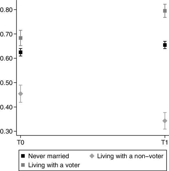
Figure 1. Turnout at T0 and T1 for never married, lives with a potential nonvoter, and lives with a potential voter. T0 is before living together (if doing so), and T1 is when living together (if doing so). BHPS and UKHLS. Fixed effects for election year.
The likelihood of voting before and after entering a relationship
Figure 2 shows the predicted probabilities of voting using difference-in-differences estimations from three balanced panels.Footnote 20 T1 shows the predicted probabilities of voting in the first election after entering a relationship, T0 shows the predicted probabilities of voting in the election before entering a relationship, T1 and T2 add observations from previous elections. The low number of respondents in the longer panel calls for caution when interpreting the results. Nevertheless, the results do not indicate that the individuals who entered relationships with eventual voters and the individuals who entered relationships with potential nonvoters had remarkably different trends in turnout over time before they entered the relationships.

Figure 2. Predicted probabilities of voting. T0 is the last election before entering a relationship and T1 is the first election after entering a relationship. Panel 1 (n = 3031, clusters=1516), panel 2 (n = 1569, clusters=523), panel 3 (n = 744, clusters=186). BHPS and UKHLS.
Table 2 shows the results from a difference-in-difference analysis with data limited to the respondents who were single at T0 and are married or cohabiting at T1 (and whose partner answered the survey at T1). Model 1 in Table 2 shows the results from a model using the unmatched data, and model 2 uses matched samples. We can now see that there are substantial differences in the change between the individuals who entered a relationship with a potential voter compared to the individuals who entered a relationship with a potential nonvoter. Entering a relationship with a potential voter increases one’s likelihood of voting while entering a relationship with a potential nonvoter decreases one’s likelihood of voting. Regardless of the modeling choice, matched or unmatched data, the individuals who entered a relationship with potential nonvoters are less likely to vote after they enter a relationship and the individuals who entered relationships with potential voters are more likely to vote after they enter a relationship. The increase in the difference between the groups is somewhat larger in the model that uses matched samples. In other words, when observations are removed where selection is most likely, and the difference between the groups is closer to what would have been the case if randomization were possible, the increase in the difference is somewhat larger. Most importantly, regardless of the choice of estimation method, the increase in the difference between the groups is substantial. The smallest estimation of the effect, using unmatched data, is as large as 23 percentage points.
Table 2. Difference in differences and predicted probabilities of voting

95% confidence intervals in brackets
Predicted probabilities to vote. Living together with voter. BHPS and UKHLS
In sum, the results support previous studies indicating that there is a social element of voting participation. The respondents who entered relationships with eventual voters had an increase in turnout, whereas the respondents who entered relationships with potential nonvoters had a decrease in turnout. The increase in the difference in turnout levels between the groups is substantial, and the difference is robust to a variation of modeling strategies. The results are in line with previous research finding spill-over effects of mobilization (Nickerson, Reference Nickerson2008) and a positive relationship between having a partner who votes and turning out to vote in the US (Stoker and Jennings, Reference Stoker and Jennings1995) and in Europe (Bhatti et al., Reference Bhatti, Fieldhouse and Hansen2018). However, there is also selection into the relationships with voters and nonvoters. The following section studies the selection into such relationships.
Socioeconomic inequalities in social influence
The larger the share of voters in the population, the larger is the chance to be influenced positively by other people who vote (Fowler, Reference Fowler and Zuckerman2005). In the case of mating, it would thus be expected that the higher the aggregate turnout, the more common it is to enter a relationship with a potential voter. This argument can be extended to a discussion of political inequalities. As turnout differs between socioeconomic groups, and mating is often based on homogamy, these self-reinforcing patterns may exist not only on the aggregate level but also between socioeconomic groups. The more likely one is to enter a relationship with a voter the more likely one is to vote in the future. In other words, turnout inequality between socioeconomic groups may be reproduced through the process of mating. To test this argument, I study the selection into relationships with eventual voters and nonvoters, as well as whether a change in behavior is conditional on socioeconomic status.
Figure 3 presents the predicted probabilities of entering a relationship with an eventual voter for previous nonvoters and previous voters at different levels of education and income.Footnote 21 The results show that regardless whether individuals voted or not in the last election, highly educated and high-income individuals are more likely to enter a relationship with an eventual voter. Individuals who are less educated and have lower income, however, are less likely to enter a relationship with an eventual voter, especially if they themselves are previous nonvoters. The differences between the socioeconomic groups are not only statistically significant but also substantial. The likelihood that a previous nonvoter with primary education enters a relationship with a potential voter is approximately 31 percent while the likelihood that a previous nonvoter with a higher degree enters a relationship with an eventual voter is as high as approximately 57 percent. In the case of previous nonvoters, the difference between the income groups is similar in size. However, among the previous voters, the probability of entering a relationship with an eventual voter does not differ much across income groups.

Figure 3. Probability of entering a relationship with a potential voter for previous nonvoters and voters by education and monthly income. BHPS and UKHLS.
Another aspect than the probability of entering a relationship with an eventual voter or nonvoter that is of importance to answer the question of a possible self-reinforcing pattern of political inequality is the question of heterogeneous changes in behavior. Although the probability of entering a relationship with a potential voter or nonvoter is dependent on one’s own socioeconomic status, the question of whether such patterns would actually reproduce political inequalities is also dependent on the change in probability of voting not being homogeneous or larger among highly educated and high-income individuals. If, however, the size of the change in the probability of voting is substantially larger among less educated, lower-income individuals, this may reduce inequalities in voting participation between the socioeconomic groups.
Figure 4 presents results estimated from models with three-way interactions between time, turnout, and education/income.Footnote 22 In other words, the change is interacted with either education or income. The other variables are included as covariates, and the model includes fixed effects for election year. For education, it appears to be no differences in the size of the change between socioeconomic groups, while among the income groups, there is a tendency that the higher-income individuals are more affected by entering a relationship with a potential voter. Thus, the difference in the probability of voting, before and after entering a relationship, between individuals who’s partners are potential voters, and nonvoters is larger among individuals with high socioeconomic status.
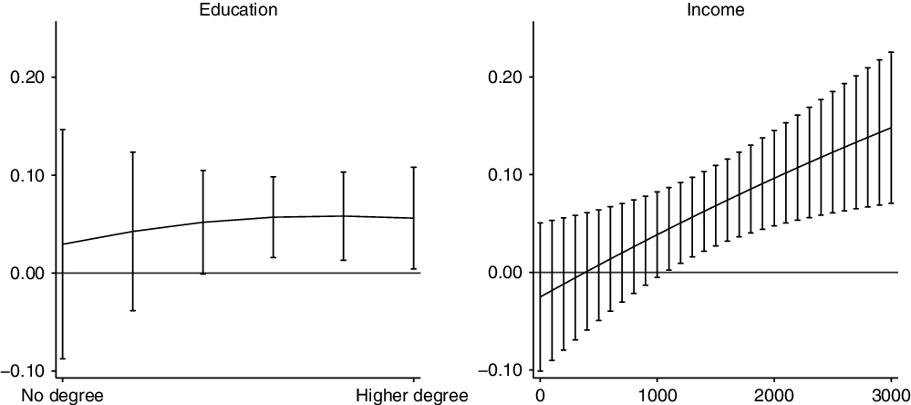
Figure 4. Difference in changes of likelihood to vote when entering a relationship with an eventual voter, by education and income groups. BHPS and UKHLS.
In sum, there are substantial differences between the likelihood of entering a relationship with a potential voter depending on one’s own education and income levels. These differences can be seen as support for the hypothesis that self-reinforcing patterns of turnout exist not only at the aggregate level but also between socioeconomic groups. In addition, the change in the likelihood of turnout of individuals who enter relationships with eventual voters is larger among the individuals with higher incomes.
Discussion
Combining theories of the social aspects of voting with insights from literature on assortative mating and literature on socioeconomic inequalities in turnout, this paper shows that assortative mating can reproduce unequal turnout. The results show that individuals who enter relationships with eventual voters increase their likelihood of voting and individuals who enter relationships with eventual nonvoters decrease their likelihood of voting. Moreover, the findings show that the likelihood of entering a relationship with an eventual voter is highly dependent on an individual’s socioeconomic status. Regardless of their own previous voting participation, the highly educated and rich individuals are substantially more likely to enter a relationship with an eventual voter than are less educated and low income individuals. In addition, the predicted increase in the probability of voting when entering a relationship with an eventual voter is larger among the individuals with high income.
This paper complements previous research in several ways. The results are in line with previous research finding that marrying a voter increases one’s likelihood of voting (Stoker and Jennings, Reference Stoker and Jennings1995; Bhatti et al., Reference Bhatti, Fieldhouse and Hansen2018). Theoretically, the results support the idea of a social mobilizing effect (a spill-over effect, a companion effect, or a contagion effect) (Gerber et al., Reference Gerber, Green and Larimer2008; Nickerson, Reference Nickerson2008; Fieldhouse and Cutts, Reference Fieldhouse and Cutts2012; Rolfe, Reference Rolfe2012; Sinclair et al., Reference Sinclair, McConnell and Green2012; Bhatti et al., Reference Bhatti, Dahlgaard, Hansen and Hansen2017) and a social demobilizing effect (Partheymüller and Schmitt-Beck, Reference Partheymüller and Schmitt-Beck2012) in the case of marriage and cohabitation. Moreover, showing that both selection into, and the social influence in relationships, matter for who participates in politics, the paper adds valuable insights to the longstanding debate on selection versus social influence (Kandel, Reference Kandel1978; Huckfeldt and Sprague, Reference Huckfeldt and Sprague1987; Jennings and Stoker, Reference Jennings, Stoker and Zuckerman2005; Alford et al., Reference Alford, Hatemi, Hibbing, Martin and Eaves2011).
The results show that previous nonvoters with high education and income are more likely to enter relationships with potential voters than previous nonvoters with less education and income. In other words, regardless of one’s previous turnout, the higher the education and income, the more likely one is to enter a relationship with a potential voter, and the less education and income, the more likely one is to enter a relationship with a potential nonvoter. This result is in line with previous research finding a positive relationship between the education level of an individual’s partner and individual turnout (Knack, Reference Knack1992; Stadelmann-Steffen and Koller, Reference Stadelmann-Steffen and Koller2014; Frödin Gruneau, Reference Frödin Gruneau2018). In other words, the use of panel data leads us one step closer to identifying a self-reinforcing pattern of political inequality. Previous research makes theoretical suggestions that mating can be seen as a large-scale GOTV experiment with unequal distribution of treatment (Frödin Gruneau, Reference Frödin Gruneau2018) and that the likelihood of being affected by a contagion effect is dependent on the aggregate turnout level (Fowler, Reference Fowler and Zuckerman2005). In addition, the results show that previous nonvoters with higher income are more likely than the individuals with lower income to change their turnout behavior when entering a relationship with an eventual voter and that previous nonvoters in different education groups are equally likely to change their behavior when entering such a relationship. In other words, this paper finds that the likelihood of receiving the “treatment’’ of entering a relationship with a potential voter and the size of such “treatment effect’’ are dependent on one’s socioeconomic status. Thus, the results indicate that a self-reinforcing pattern of turnout may be present not only at the aggregate level but also within socioeconomic groups.
There are some limitations to this study. First, the design of the study does not allow making distinctions between possible mechanisms that can explain the relationship between entering a relationship with a potential voter and one’s own turnout. There are several suggestions in the previous literature that could explain an increase in turnout when entering such a relationship. For example, scholars have ascribed the act of voting to individuals who have a great sense of civic duty. It could be the case that individuals who enter relationships with potential voters develop a sense of civic duty (Knack, Reference Knack1992). Another possible mechanism could be that individuals who enter relationships with potential voters increase their political interest. The individuals who enter relationships with potential voters might be more likely to vote because they have been more exposed to political discussion with their partner (Beck, Reference Beck1991). Another explanation could be, a companion effect, that voting is a social activity that people who live together are likely to engage in together (Fieldhouse and Cutts, Reference Fieldhouse and Cutts2012). Unfortunately, the study at hand cannot answer why individuals who enter relationships with potential voters become more likely to vote nor why individuals who enter relationships with potential nonvoters become less likely to vote. However, the different mechanisms are neither unrelated nor exclusive.
Second, empirically identifying what theoretically is a causal story using the case of mating, a societal process with a large degree of selection, is not ideal. For example, using the panel data from a household panel, I do not have information on the voting participation of the partner before entering the relationship. Assigning the ’’treatment’’ based on the post facto voting participation of the partner is not ideal, and I cannot determine the relative importance of who influences whom in the relationship. If the aim had been primarily to identify causality or mechanisms, an identification strategy closer to an experiment would have been necessary. Recently, such identification strategies have become more common in political science. There are examples of researchers successfully identifying a social element of mobilization (Nickerson, Reference Nickerson2008; Gerber et al., Reference Gerber, Green and Larimer2008) and showing that a spouse who votes is a great mobilizing force (Hobbs et al., Reference Hobbs, Christakis and Fowler2014). However, such studies will most likely have limitations when it comes to external validity. This study contributes by studying the consequences of the previously identified social mechanism of turnout by applying the theoretical framework of social mobilization to the case of marriage and cohabitation. The main point here is that the selection process of mating itself is important for understanding who participates in politics. Given that there is a social aspect of political mobilization the structure for who marries whom matters for who participates in politics.
This paper identifies fruitful avenues for future research, such as identifying the mechanisms that can explain the relationship between entering a relationship with a potential voter and one’s own voting participation. Forming a better understanding of the mechanisms may also lead to better understanding of why, and when, individuals of different socioeconomic groups are more or less likely to change their behavior when entering a relationship. In addition, this study uses the British case. Although the social aspects of mobilization have been studied in other contexts, the question of who enters a relationship with a potential voter has not. Theoretically, there is no reason to suspect that the findings are exclusive to the British case. However, there are good reasons to believe that the degree of unequal exposure to potential voting companions varies across contexts. The theories of mating suggest that who you marry is dependent on choice and on who you are likely to meet. The likelihood of marrying a voter among the rich and highly educated and among the less educated with lower income may thus be dependent on the social structure and may vary by context. In other words, if a nonvoter with less education were just as likely as a nonvoter with high education to be influenced by social mobilization to vote, this process could reduce inequalities in turnout. If that is the case, such a process could help to explain decreased differences in turnout between men and women over time. When mating on heterogeneity (women-men) instead of homogeneity (high education-high education) is the norm, inequalities between groups would be expected to decrease over time.
The main takeaway here is that mating processes can reproduce the difference in turnout between socioeconomic groups, as the likelihood of entering relationships with voters differ depending on socioeconomic status. The results indicate that what has previously been discussed as an aggregate-level self-reinforcing process of turnout (Fowler, Reference Fowler and Zuckerman2005; Nickerson, Reference Nickerson2008) can also be found within socioeconomic groups. In groups where turnout is low, such as among individuals with low education and low income, the likelihood of marrying a voter is low. In groups where turnout is high, such as among individuals with high education and income, the likelihood of marrying a voter is high. In other words, if turnout among one’s likely mates is low, it is likely to stay low, and if turnout among one’s likely mates is high, it is likely to stay high. Thus, the combination of assortative mating and social influence in turnout can support a self-reinforcing pattern of political inequality.
Acknowledgements
The author thanks Jenny de Fine Licht, Mikael Persson, Johanna Rickne, seminar participants at the annual meeting of the Swedish Political Science Association (2017), Midwest Political Science Association (2018), the Elections, Public Opinion and Parties conference (2018), the Gothenburg Politics and Gender workshop (2018), the Uppsala Politics and Gender seminar (2018), and three anonymous reviewers for feedback on previous versions of this paper.
Supplementary material
To view supplementary material for this article, please visit https://doi.org/10.1017/S1755773920000016


 Open access