


1. Introduction
Wind gustiness is a ubiquitous phenomenon in the atmospheric boundary layer. When the gustiness is strong, the variation in the wind speed becomes comparable to the average value, which has significant effects on air–sea interactions. In weather and climate models, the wind gustiness parametrization is important because computations based on the average wind speed can underestimate the air–sea fluxes significantly, especially when the mean wind speed is low (Zeng et al. Reference Zeng, Zhang, Johnson and Tao2002). Additionally, the wind gustiness may affect the upper ocean temperature (Giglio et al. Reference Giglio, Gille, Subramanian and Nguyen2017) and the fluctuations in the electricity power output generated by wind turbines (Stevens & Meneveau Reference Stevens and Meneveau2017).
For the interaction between wind and waves, the gustiness effect is often found to be non-negligible. In a laboratory experiment, Waseda, Toba & Tulin (Reference Waseda, Toba and Tulin2001) investigated wave evolution in a water tank by imposing a sudden change in wind speed. They identified the deviation from the  $3/2$ power law (Toba Reference Toba1972) that indicates a local wind–wave equilibrium state, i.e.
  $H_s \propto (gu_*)^{1/2}T_s^{3/2}$, where
  $H_s$ is the significant wave height,
  $u_*$ is the air friction velocity and
  $T_s$ is the significant wave period. Their results also showed hysteresis in the wave height responses to increasing and decreasing wind. Abdalla & Cavaleri (Reference Abdalla and Cavaleri2002) used a random sequence to model the wind speed fluctuations, which was incorporated into the wind input source term in an operational phase-averaged wave model (Komen et al. Reference Komen, Cavaleri, Donelan, Hasselmann, Hasselmann and Janssen1994). Abdalla & Cavaleri (Reference Abdalla and Cavaleri2002) then performed a series of simulations, including idealized runs based on prescribed physical conditions, and practical runs based on historical data from meteorological observations. Their results showed that the gustiness effects on slow waves are limited, while for fast waves, a gusty wind field can enhance significantly the wave growth compared with that under constant winds. Annenkov & Shrira (Reference Annenkov and Shrira2011) investigated numerically the evolution of a nonlinear wave field, and found that the integral wave properties under a gusty wind forcing are consistent with those under an effective constant wind forcing. It should be noted that the sources of the gustiness used in the above two modelling-based studies are different. Abdalla & Cavaleri (Reference Abdalla and Cavaleri2002) considered the variations in the observable wind speed. Annenkov & Shrira (Reference Annenkov and Shrira2011) modelled the gustiness by adjusting the wave energy growth rate, which is challenging, generally, to measure directly from observations. In a field study, Hwang, García Nava & Ocampo-Torres (Reference Hwang, García Nava and Ocampo-Torres2011) observed that the wave energy growth in unsteady wind forcing is quantitatively different from that in a steady forcing. Their results also provide evidence of the hysteresis effect of wave development, namely, a much slower rate of change of the characteristic wave properties in decaying wind speed than in the growing wind. More recently, Zavadsky & Shemer (Reference Zavadsky and Shemer2017) performed a laboratory experiment to investigate the initial wave generation from a quiescent surface under impulsive wind forcing. Model development for gustiness effect is still at an early stage. In the European Centre for Medium-range Weather Forecasts (ECMWF) model (ECMWF 2020), the gustiness impact is parametrized through a simple model mainly to enhance the wind energy input to waves.
While the past several decades saw a growing number of studies on wind–wave interaction, most of the theoretical and numerical studies assumed that the wind turbulence is statistically stationary. In the quasi-laminar model proposed by Miles (Reference Miles1957), the wind field is simplified as the superposition of a prescribed mean profile and wave-induced resonant motions, while the effects of turbulence and viscosity are neglected. The critical layer was found to play a dominant role in wave growth, which has been substantiated by field observations (Hristov, Miller & Friehe Reference Hristov, Miller and Friehe2003). Belcher & Hunt (Reference Belcher and Hunt1993) considered the turbulence impact on the wave growth through the non-separated sheltering mechanism, which was found to be important for slow waves. Nikolayeva & Tsimring (Reference Nikolayeva and Tsimring1986) and Miles & Ierley (Reference Miles and Ierley1998) considered the effect of wind gustiness in the study of wave growth. But in both studies, the mean wind velocity profiles were assumed to be slowly varying in time, and the transient dynamics were neglected in the equivalent steady flow. In canonical numerical configurations (e.g. Sullivan, Mcwilliams & Moeng Reference Sullivan, Mcwilliams and Moeng2000), the wind turbulence field is simulated over a monochromatic travelling wave, and this framework has been used widely to explore the steady-state features of turbulent flows in wind–wave interactions. For example, Kihara et al. (Reference Kihara, Hanazaki, Mizuya and Ueda2007) studied the dependence of wave-coherent motions on the wave age. Yang & Shen (Reference Yang and Shen2010) showed a significant impact of wave on the near-surface coherent vortical structures. Based on the transformed Navier–Stokes equations on a boundary-fitted grid, Hara & Sullivan (Reference Hara and Sullivan2015) derived a momentum balance equation and elucidated the role of the wave-induced stresses. Recently, Åkervik & Vartdal (Reference Åkervik and Vartdal2019) proposed an approach to split the wind field into a shear flow and a wave-induced part. The linear solution obtained using this method was found to capture the main features of the flow in the cases with high wave ages, but large deviations were observed at low wave ages. They also found that the nonlinear solution, which takes account of turbulence forcing, is in close agreement with the large-eddy simulation (LES) results in both cases. Cao, Deng & Shen (Reference Cao, Deng and Shen2020) developed a viscous curvilinear model to predict the wave-coherent motions based on the mean wind velocity profile and the wave orbital velocity. The model shows excellent performance when applied to wind over opposing waves and wind over fast following waves, while for wind over slow following waves, notable discrepancies between the model prediction and the simulation results were observed (Cao et al. Reference Cao, Deng and Shen2020; Cao & Shen Reference Cao and Shen2021). Husain, Hara & Sullivan (Reference Husain, Hara and Sullivan2022a,Reference Husain, Hara and Sullivanb) performed numerical experiments of wind turbulence when the waves are travelling at an oblique angle to the wind direction, and they identified a strong impact of the oblique angles on the air–sea momentum flux. In the studies reviewed above, the wind field is typically driven by a constant pressure gradient in the domain or a constant velocity or shear stress at the domain top, and the resulting turbulence statistics are stationary in time. Therefore, the wind–wave energy transfer is determined by the steady-state variables, such as the characteristic wind speed and the characteristic wave properties.
Some recent simulation-based studies have also investigated more complex physical processes by taking into account the spatial/temporal heterogeneity in the wind–wave system. For example, Yang, Deng & Shen (Reference Yang, Deng and Shen2018) studied the wind turbulence over breaking waves, and elucidated the transient and non-equilibrium features of the turbulence locally in space and time. Irregular broadband wave fields have also been used in the problem set-up of several studies (Sullivan, McWilliams & Patton Reference Sullivan, McWilliams and Patton2014; Wang et al. Reference Wang, Zhang, Hao, Huang, Shen, Xu and Zhang2020), although the temporal variation of the mean profile was not considered. Dynamically coupled wind–wave evolution was studied recently by Hao & Shen (Reference Hao and Shen2019). In that study, the pressure gradient used to drive the wind field was constant, and because the characteristic time scale of the nonlinear wave evolution was considerably larger than the wave periods, the wind turbulence field was largely statistically stationary in time. In experimental studies, it is also common practice to maintain a certain wind speed (e.g. Liberzon & Shemer Reference Liberzon and Shemer2011; Grare et al. Reference Grare, Peirson, Branger, Walker, Giovanangeli and Makin2013; Yousefi, Veron & Buckley Reference Yousefi, Veron and Buckley2020). While spatial heterogeneity may appear in the water tank because of wave evolution downstream (Zavadsky & Shemer Reference Zavadsky and Shemer2012) and airflow separation (Buckley, Veron & Yousefi Reference Buckley, Veron and Yousefi2020), the wind turbulence field is statistically stationary.
In summary of the reviews above, our knowledge on the non-stationary turbulence features in wind–wave interaction subject to wind gustiness is rather limited. In the present study, we investigate the response of an initially steady wind field above a prescribed wave to a growing/decaying wind gust event. Our objective is to elucidate the key airflow transient processes, including the evolution of turbulence and wave-coherent motions. We also study the change in the wind–wave energy transfer associated with the gust, and explore the underlying mechanisms. To achieve this goal, we perform LES of the wind turbulence on a wave-boundary-fitted grid, a numerical framework that has been validated in various studies (e.g. Yang & Shen Reference Yang and Shen2011a,Reference Yang and Shenb; Hao & Shen Reference Hao and Shen2019; Cao et al. Reference Cao, Deng and Shen2020). We do not consider the wave evolution during the wind gust because the time scale of the wind gust is only a few wave periods, and it has been shown that the time scale for the wave to have noticeable change is much larger (Annenkov & Shrira Reference Annenkov and Shrira2011). The remainder of this paper is organized as follows. In § 2, we introduce the simulation configuration and the case design. In § 3, we present results on the overall wind field evolution (§ 3.1), the transient features of the turbulent stresses (§ 3.2), the wave-coherent motions (§§ 3.3 and 3.4) and the wave growth rate (§ 3.5). Finally, conclusions are given in § 4.
2. Methodology and problem set-up
2.1. Large-eddy simulation on a boundary-fitted grid
Following our previous work (Hao & Shen Reference Hao and Shen2019), the wind turbulence is simulated using wall-resolved LES. The governing equations for the air motions are written as
 \begin{gather} \frac{\partial {u}_i}{\partial x_i}=0, \end{gather}
 \begin{gather} \frac{\partial{u}_i}{\partial t}+{u}_j\,\frac{\partial{u}_i}{\partial x_j} ={-}\frac{1}{\rho}\,\frac{\partial {p}}{\partial x_i} -\frac{\partial\tau_{ij}^{d}}{\partial x_j}+\nu\,\frac{\partial^{2} u_i} {\partial x_j\,\partial x_j} +B(t)\,\delta_{i1}, \end{gather}
where  ${u}_i (i=1,2,3)=({u},{v},{w})$ denotes the filtered velocity in LES,
  $p$ is the filtered modified pressure,
  $\tau _{ij}^{d}$ is the trace-free part of the subgrid-scale (SGS) stress tensor,
  $\rho$ is the air density,
  $\nu$ is the kinematic viscosity of air,
  $B(t)$ denotes the driving force used for the flow rate control, and
  $x$,
$x$,  $y$ and
  $z$ denote the streamwise, spanwise and vertical coordinates, respectively. The domain sizes are denoted by
  $L_x$,
  $L_y$ and
  $L_z$. The schematic of the computational domain is shown in figure 1(a).

Figure 1. Sketch of (a) the computational domain, and the flow rate  $Q(t)$ response to the driving force
  $B(t)$ in (b) the growing wind and (c) the decaying wind.
To account for the geometric deformation caused by the wave profile, the LES governing equations are solved on a wave surface boundary-fitted grid via a transformation from the physical space  $(x,y,z,t)$ to the computational space
  $(\xi,\psi,\zeta,\tau )$. The details of the grid transformation and the numerical solver are provided in Appendix A. Here we give an overview of the numerical scheme. Details can be found in Yang & Shen (Reference Yang and Shen2011a,Reference Yang and Shenb). At each time step, the spatial derivatives in the horizontal directions are calculated using Fourier transforms, and those in the vertical direction are calculated using second-order finite differences. The SGS stress tensor is calculated using the dynamic Smagorinsky model (Smagorinsky Reference Smagorinsky1963; Germano et al. Reference Germano, Piomelli, Moin and Cabot1991; Lilly Reference Lilly1992). The momentum equation is first advanced in time without the pressure term to obtain the interim velocity field. The Poisson equation for the pressure is then solved, and the pressure field is used to correct the velocity field to satisfy the continuity equation. The second-order Adam–Bashforth scheme is used for time advancement. The simulation starts from randomly generated turbulent motions imposed on a logarithmic mean velocity profile, with a flat bottom boundary initially to expedite the simulation process. The wave kinematics are then incorporated into the boundary condition through a relaxation process. More details and validations of the numerical solver can be found in Yang & Shen (Reference Yang and Shen2011a,Reference Yang and Shenb), Cao et al. (Reference Cao, Deng and Shen2020) and Cao & Shen (Reference Cao and Shen2021).
In previous studies on the steady state wind–wave interaction, the wind turbulence is driven by a constant pressure gradient (e.g. Yang, Meneveau & Shen Reference Yang, Meneveau and Shen2013; Åkervik & Vartdal Reference Åkervik and Vartdal2019; Wang et al. Reference Wang, Zhang, Hao, Huang, Shen, Xu and Zhang2020), or by a constant velocity or shear stress at the top boundary of the computational domain (Sullivan et al. Reference Sullivan, Mcwilliams and Moeng2000; Druzhinin, Troitskaya & Zilitinkevich Reference Druzhinin, Troitskaya and Zilitinkevich2012; Cao et al. Reference Cao, Deng and Shen2020; Cao & Shen Reference Cao and Shen2021) to maintain a constant flow rate. To model the wind gust event, we apply a time-varying pressure gradient  $\rho B(t)$ to control the flow rate of the wind field. In the first stage of the simulation, this driving force is set to guarantee a constant flow rate, which then varies linearly in a short time duration
  $0< t< T_g$. The expression for
  $B(t)$ is
 \begin{equation} B(t)=\frac{\mathrm{d}Q}{\mathrm{d}t}\,\frac{1}{hL_y} -\frac{\tau_\nu(t)+\tau_p(t)}{\rho h}, \end{equation}
where  $h=L_z$ is the vertical domain size,
  ${\mathrm {d}Q}/{\mathrm {d}t}$ is the desired rate of change of the volumetric flow rate
  $Q$,
$Q$,  $\tau _{\nu }(t)$ is the total viscous drag at the top boundary and the wave surface, and
  $\tau _p(t)$ is the form drag at the wave surface. Generally, the second term is not a constant because
  $\tau _{\nu }(t)$ and
  $\tau _p(t)$ vary in time. However, its contribution to
  $B(t)$ is negligibly small compared with the first term in typical gust events. After the flow rate has reached the designed value, the force is assigned a different value to maintain the flow. For a growing wind,
  ${\mathrm {d}Q}/{\mathrm {d}t}$ is positive (figure 1b), while for a decaying wind,
  ${\mathrm {d}Q}/{\mathrm {d}t}$ is negative (figure 1c). The flow rate control scheme used here is similar to that in computational studies of transient turbulent channel flows (e.g. He & Seddighi Reference He and Seddighi2015), and is a close approximation to the wind speed control in laboratory studies (Waseda et al. Reference Waseda, Toba and Tulin2001; Zavadsky & Shemer Reference Zavadsky and Shemer2017).
The simulation parameters are summarized in table 1. To facilitate the decomposition of the turbulence field, we adopt the canonical set-up of wind over a prescribed monochromatic progressive wave. The wave steepness in our simulation is set to a typical value  $ak=0.05$, where
  $a$ is the wave amplitude, and
  $k$ is the wavenumber. A wide range of wave ages is selected for the initial wind–wave state, including both slow waves (e.g.
  $c/u_*=4.4$ in case CU8) at the early stage of wind–wave generation (Belcher & Hunt Reference Belcher and Hunt1993; Janssen Reference Janssen2004), and fast waves (e.g.
  $c/u_*=41.6$ in case CU42) that are typically found under swell-dominated sea conditions (Sullivan et al. Reference Sullivan, Edson, Hristov and McWilliams2008). Following previous wind–wave studies (Henn & Sykes Reference Henn and Sykes1999; Calhoun, Street & Koseff Reference Calhoun, Street and Koseff2001; Yang et al. Reference Yang, Meneveau and Shen2013), we use a computational domain
  $(L_x, L_y, L_z)=(2\lambda, \lambda, \lambda )$, where
  $\lambda$ is the wavelength. The domain size in the streamwise direction enables the simulation of turbulence coherent motions larger than
  $\lambda$, and is sufficiently large to produce the correct temporal correlation in the turbulence statistics (Hao, Cao & Shen Reference Hao, Cao and Shen2021). The grid number is
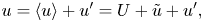
  $N_x\times N_y\times N_z=128\times 256\times 96$. To capture accurately the turbulent motions of the smallest eddies in the simulation, we choose the appropriate initial and final Reynolds numbers such that the grid resolutions satisfy the criterion of wall-resolved LES (Choi & Moin Reference Choi and Moin2012). Note that the final Reynolds number in table 1 corresponds to the new equilibrium state of the wind turbulence after the simulations are performed for a sufficiently long time after the wind gust ends. The simulations are performed in the fixed frame of reference, and in the following analysis related to wave-coherent motions, a frame translating with velocity
  $(c,0,0)$ is considered.
Table 1. Numerical parameters of the simulations. Here,  $c^{+}$ is the ratio of the wave phase velocity to the instantaneous friction velocity
  $u_*$, also known as the wave age,
  ${\textit {Re}}_{\tau }$ is the Reynolds number based on the friction velocity and the wavelength
  $\lambda$,
  $(N_x, N_y, N_z)$ are the grid numbers, and
  $(\Delta \xi ^{+}, \Delta \psi ^{+}, \Delta \zeta _{min}^{+})$ are the sizes of the first grid above the wave surface, normalized in wall units. Note that
  $\Delta \xi ^{+}$ and
  $\Delta \psi ^{+}$ are the effective values after accounting for de-aliasing in the Fourier spectral method.

The time scales of the wind gust are summarized in table 2. The wind gust duration  $T_g$ is a few wave periods. Since there is no rigorous definition of a wind gust duration,
  $T_g$ is assumed equivalent to a dimensional time scale of
  $O(1-10)$ s and therefore agrees with the 20 s limit adopted by the U.S. National Weather Service and the 3 s standard recommended by World Meteorological Organization (WMO) (2018). According to the wave tank experiment of Waseda et al. (Reference Waseda, Toba and Tulin2001), the initial adjustment time of slow waves (
 $c/u_*=1-1.5$) responding to the wind gust event is
  $15T\unicode{x2013}20T$. They also showed that for a field case (
 $c/u_*=9$), this time scale becomes
  $210T\unicode{x2013}420T$. In the following analysis, we focus on a short period during and after the wind gust event. Therefore, the changes in the wave properties can be neglected.
Table 2. Time duration of the wind gust event  $T_g$, normalized by the wave period
  $T$ and the largest eddy turnover time
  $h/u_*$.

For each case shown in table 1, the growing and decaying wind gust events are simulated separately. We first perform the simulation at the initial Reynolds number, and after a statistically stationary state is reached, we impose a gust event on the steady wind turbulence field by varying the driving force  $B(t)$ as described in (2.3) and shown in figure 1(b). Because of the rapid gust event, the wind turbulence field is non-stationary and no longer ergodic. It is therefore inappropriate to approximate the Reynolds averaging with the time averaging during this period. To address this issue, we perform 50 ensemble runs for each simulation, so that the turbulence statistics can be calculated but with a substantially increased computational cost. Note that for the above reason, some statistical results are less smooth compared to the steady setting where time averaging can be performed, but this does not affect the conclusions of the analyses.
2.2. Triple decomposition and normalization
In the following analyses, the turbulence field is decomposed into three parts (Hussain & Reynolds Reference Hussain and Reynolds1972):
 \begin{equation} u=\langle u\rangle+u'=U+\tilde{u}+u', \end{equation}
where  $U$ denotes the mean profile,
  $\tilde {u}$ denotes the wave-coherent motions, and
  $u'$ is the ‘pure’ turbulent motion. The operator
  $\langle \cdot \rangle$ is defined by the phase average of all ensemble simulations,
 \begin{equation} \langle u\rangle(\xi,\zeta,t)=\frac{1}{NN_y}\sum_{n,j} u_n(\xi-ct,y_j,\zeta,t), \end{equation}
where  $u_n$ is the instantaneous quantity in the
  $n$th simulation (
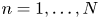 $n=1,\ldots, N$;
  $N=50$). The phase-shift operation can be calculated conveniently via Fourier transform.
At each constant  $\zeta$, a wave-coherent component (take
  $\tilde {u}$ as an example) can be written as
 \begin{equation} \tilde{u}(x,t)=\mathrm{Re}[\tilde{u}](t)\cos(kx)-\mathrm{Im}[\tilde{u}](t)\sin(kx), \end{equation}
where  $\mathrm {Re}[\tilde {u}]$ and
  $\mathrm {Im}[\tilde {u}]$ are the real and imaginary parts of the Fourier coefficient, respectively. Traditionally,
  $\mathrm {Re}[\tilde {u}]\cos (kx)$ and
  $\mathrm {Im}[\tilde {u}]\sin (kx)$ are also called the in-phase and out-of-phase components, respectively (e.g. Belcher & Hunt Reference Belcher and Hunt1993). An alternative form is
 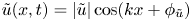 $\tilde {u}(x,t)=|\tilde {u}|\cos (kx+\phi _{\tilde {u}})$, where
  $|\tilde {u}|=(\mathrm {Re}[\tilde {u}]^{2}+\mathrm {Im}[\tilde {u}]^{2})^{1/2}$ and
  $\phi _{\tilde {u}}=\tan ^{-1}(\mathrm {Im}[\tilde {u}]/\mathrm {Re}[\tilde {u}])$ are the amplitude and phase of
  $\tilde {u}$, respectively. With respect to the wave profile, the real (imaginary) part, i.e. the in-phase (out-of-phase) component, corresponds to the symmetry (anti-symmetry) on the two sides of the wave crest.
Because of the gust events, the near-wall turbulence states, including the wall stress and the friction velocity, are non-stationary. In the following analyses, we use two types of scaling for normalization. Quantities with the superscript ‘ $+$’ are normalized in the instantaneous time-variant wall units. In the second type of scaling, we introduce the superscripts ‘
 $+0$’ to denote the time-invariant normalization under the initial turbulent flow condition in the growing wind, and the corresponding friction velocity is denoted by
  $u_{*,0}$.
3. Results
3.1. Overview of wind turbulence field evolution
In this section, we first give an overview of the wind field evolution with a focus on the turbulent motion ( $u', v', w'$) defined in (2.4). For the length consideration of the paper, we present results in the growing wind of case CU8 when the flow dynamics are similar among the different cases in table 1. Figure 2 shows
  $u'$ and
  $w'$ at the start and end of the growing wind gust. The magnitude of
  $u'$ is generally stronger than
  $w'$ at both
  $t=0$ and
  $t=T_g$, as shown by their contours on the
  $x$–
$x$– $z$ and
  $y$–
$y$– $z$ planes. The streaks near the wave surface, denoted by the isosurfaces of
  $u'$, are enhanced significantly after the impact of the wind gust. On the other hand, the isosurfaces of
  $w'$ at
  $t=0$ and
  $t=T_g$ are qualitatively similar. Explanations for these differences are provided from the analyses in § 3.2.

Figure 2. Turbulent motions at (a,b)  $t=0$ and (c,d)
  $t=T_g$ for the growing wind in case CU8. Plotted are the contours of
  $u'$ and
  $w'$ on the
  $x$–
$x$– $z$ and
  $y$–
$y$– $z$ planes, and the isosurfaces corresponding to
  $u'^{+0}=\pm 7$ in (a,b) and
  $w'^{+0}=\pm 3$ in (c,d), where the superscript ‘
 $+0$’ denotes the normalization based on the wall unit at the initial state (see table 1).
The mean wind profiles before, during and shortly after the gust event are plotted in figure 3. During the gust event  $0< t/T_g<1$, the mean flow away from the wave surface (
 $\zeta >0.01\lambda$) experiences a similar change and the velocity profiles are shifted by a roughly constant value. The dominant mechanism can be understood through the averaged streamwise momentum equation, which reduces to
  $\partial U/\partial t=B(t)$ to the leading order. Since
  $B(t)$ is nearly a constant, the time variation in the mean profile is linear and uniform. While a logarithmic region remains in the mean profile at the end of the gust
  $t=T_g$, the wind turbulence is in a non-equilibrium state. Therefore, the slope of the mean profile is no longer determined only by the friction velocity, and the mean profile cannot be used to calculate the wave growth rate in the same way as when the wind turbulence is steady (Miles Reference Miles1957; Belcher & Hunt Reference Belcher and Hunt1993) or quasi-stationary (Miles & Ierley Reference Miles and Ierley1998). In the region near the wave surface
  $\zeta <0.01\lambda$, the velocity gradient (i.e. the mean shear) changes significantly during the gust because of the boundary condition constraint imposed by the wave surface (see Appendix B). After the gust event, the wind field continues to evolve (comparing the profiles at
  $t=T_g$ and
  $t=1.5T_g$ in figure 3) and a new equilibrium state can be established after a sufficiently long time. Compared with the wind gust event, the temporal variations in the wind field after
  ${O}(2T_g\unicode{x2013}4T_g)$ are less drastic in the return to equilibrium and therefore excluded from the following analysis.

Figure 3. Evolution of the mean wind velocity profiles in (a) the growing wind and (b) the decaying wind, in case CU8. The profiles are normalized in the initial wall unit and plotted during  $0\leq t/T_g\leq 1.5$. The black dashed line denotes
  $U=c$.
The response of turbulence to the wind gust is in sharp contrast to that of the mean velocity profile. Figure 4 shows the profiles of Reynolds stress components at several time instants during and after the wind gust event in case CU8. Here,  $\langle v'v'\rangle$ is not plotted because its evolution is qualitatively similar to
  $\langle w'w'\rangle$. When the growing wind gust occurs (
 $0< t< T_g$), we observe a rapid increase in the streamwise velocity fluctuations
  $\langle u'u'\rangle$ (figure 4a), while
  $\langle w'w'\rangle$ (figure 4b) has relatively stable values, and the evolution speed of
  $\langle u'w'\rangle$ (figure 4c) is between those of
  $\langle u'u'\rangle$ and
  $\langle w'w'\rangle$. At
  $t=1.5T_g$, the magnitudes of all these Reynolds stress components become significantly larger as the turbulence field continues to evolve. In the decaying wind (figure 4d–f), the responses of the turbulent stress first appear near the wave surface and then extend to the outer region. These results are similar to the pipe flow experiment of accelerating and decelerating turbulence (He & Jackson Reference He and Jackson2000). The behaviours of the turbulent stresses are related closely to the gust-induced change in the mean shear. As shown above, the mean velocity profile exhibits a linear and uniform time variation such that the mean shear remains constant in the outer region and changes drastically only near the wave surface.

Figure 4. Vertical distribution of the Reynolds stresses for (a–c) the growing wind and (d–f) the decaying wind, in case CU8.
The evolution of the Reynolds stresses is also demonstrated by tracking their peak values in time, shown in figure 5. Here, we also plot the time variation of the mean flow energy  $U^{2}(t)/U^{2}(0)$ in the region
  $\zeta >0.01\lambda$. As expected, the mean flow sees a real-time response with the onset of the gust. The peak streamwise turbulence variation
  $\langle u'u'\rangle _{p}=\max {\langle u'u'\rangle }$ changes rapidly after a short delay. When the wind is growing, an overshoot appears in
  $\langle u'u'\rangle _{p}$ after the gust ends, and its temporal evolution is qualitatively similar to the channel flow result (He & Seddighi Reference He and Seddighi2015). The other two components,
  $\langle w'w'\rangle _{p}$ and
  $\langle -u'w'\rangle _{p}$, experience relatively less change in the growing and decaying wind gust. Compared with the evolution of the mean flow energy, the turbulence peak values show a delayed response (also known as the memory effect) to the gust. Because of this phase delay, the turbulent kinetic energy (TKE) relative to the mean energy, i.e.
  $\langle u_i'u_i'\rangle /U^{2}$, decreases in the growing wind and increases in the decaying wind. Detailed explanations are provided by the turbulence budget analysis in the next subsection.

Figure 5. Time variation of the peak values of the turbulence variances in (a) the growing wind and (b) the decaying wind, in case CU8. Also plotted is the mean flow energy  $U^{2}(t)$ at
  $\zeta =0.051\lambda$. All terms are normalized by their values at
  $t=0$.
3.2. Transient behaviours of a Reynolds stress budget and wave-induced effect
We perform a Reynolds stress budget analysis in this subsection to investigate the mechanism responsible for the turbulent stress evolution shown in § 3.1. In a previous study by Yang & Shen (Reference Yang and Shen2010), the budget of the TKE under the steady wind–wave condition was obtained. The detailed budget for the Reynolds stress components in unsteady wind fields over waves, however, was rarely reported. Following the work of Xuan, Deng & Shen (Reference Xuan, Deng and Shen2020) on Langmuir turbulence under waves, we can write the Reynolds stress budget equation of wind turbulence in the frame of reference moving with the wave as
 \begin{align} \frac{\partial\langle u_i' u_j'\rangle}{\partial t}&=\underbrace{-(U-c)\boldsymbol{\cdot}\boldsymbol{\nabla}\langle u_i' u_j'\rangle}_{A} +\underbrace{\nu\,\nabla^{2}\langle u_i'u_j'\rangle}_{D^{\nu}}\nonumber\\ &\quad \underbrace{{}-\langle u_i'u_k'\rangle\,\frac{\partial U_j}{\partial x_k}-\langle u_j'u_k'\rangle\,\frac{\partial U_i}{\partial x_k}}_{P^{m}} \underbrace{{}-\langle u_i'u_k'\rangle\,\frac{\partial \tilde{u}_j}{\partial x_k}-\langle u_j'u_k'\rangle\,\frac{\partial \tilde{u}_i}{\partial x_k}}_{P^{w}} \nonumber\\ &\quad \underbrace{{}-\frac{1}{\rho}\left(\frac{\partial \langle p'u_i'\rangle}{\partial x_j}+\frac{\partial \langle p'u_j'\rangle}{\partial x_i}\right)}_{T^{p}} +\underbrace{\left\langle\frac{p'}{\rho}\left(\frac{\partial u_i'}{\partial x_j}+\frac{\partial u_j'}{\partial x_i}\right)\right\rangle}_{R}\nonumber\\ &\quad \underbrace{{}-\frac{\partial \langle u_i'u_j'u_k'\rangle}{\partial x_k}-\frac{\partial \langle u_i'\tau_{jk}^{d}\rangle}{\partial x_k}-\frac{\partial \langle u_j'\tau_{ik}^{d}\rangle}{\partial x_k}}_{T^{t}} \underbrace{{}-2\nu\left\langle\frac{\partial u_i'}{\partial x_k}\,\frac{\partial u_j'}{\partial x_k}\right\rangle}_{\epsilon}, \end{align}
where  $A$ is the advection,
  $D^{\nu }$ is the viscous diffusion,
  $P^{m}$ is the production by the mean shear,
  $P^{w}$ is the production by the wave-coherent motions,
  $T^{p}$ is the pressure transport,
  $R$ is the pressure–strain correlation,
  $T^{t}$ is the spatial flux associated with turbulence and SGS stress, and
  $\epsilon$ is the dissipation. For the non-stationary turbulence field with the wind gust over the wave, each budget term is a function of two spatial coordinates (i.e.
  $\xi$ and
  $\zeta$) and the time.
To investigate the time evolution of a budget term, we perform the integration along both the  $\xi$ and
  $\zeta$ directions to evaluate its net contribution in the entire domain. For example, with the dissipation, we define
 \begin{equation} \breve{\epsilon}_{ij}(t)=\frac{1}{L_xL_z}\int \epsilon_{ij}(\xi,\zeta)\,\mathrm{d}\xi\,\mathrm{d}\zeta, \end{equation}
where the integral, denoted by  $\breve {(\ )}$, is performed in the whole computational domain (He & Seddighi Reference He and Seddighi2013); alternatively, it can be computed separately in part of the domain (Lozano-Durán et al. Reference Lozano-Durán, Giometto, Park and Moin2020), e.g. in the buffer layer and the logarithmic layer. The net contributions of the other budget terms (
 $\breve {P}_{ij}^{m}$,
  $\breve {R}_{ij}$, etc.) are calculated following (3.2).
The time history of the net contributions for  $\langle u'u'\rangle$ is shown in figure 6, where the dominant budget terms are plotted and the secondary terms are neglected for simplicity. The rapid change in the production by the mean shear
  $\breve {P}_{11}^{m}$ is a key contributor to the time variations of
  $\langle u'u'\rangle$. In both growing wind and decaying wind, there is a clear phase lag in the pressure–strain correlation
  $\breve {R}_{11}$, compared with the production
  $\breve {P}_{11}^{m}$ and the dissipation
  $\breve {\epsilon }_{11}$. The net contribution of the normal components of the pressure–strain correlation terms,
  $\breve {R}_{11}$,
  $\breve {R}_{22}$ and
  $\breve {R}_{33}$, to the TKE vanishes because their role is to redistribute the energy among the different normal Reynolds stress terms through the pressure. The direction of the energy transfer is predominantly from
  $\langle u'u'\rangle$ to
  $\langle v'v'\rangle$ and
  $\langle w'w'\rangle$, as indicated by the negative
  $\breve {R}_{11}$ in figure 6. Therefore, the delay of
  $\breve {R}_{11}$ compared with
  $\breve {P}_{11}^{m}$ explains the phase lag of
  $\langle w'w'\rangle$ with respect to
  $\langle u'u'\rangle$ (figure 5).

Figure 6. Time variation of the integrated budget terms for  $\langle u'u'\rangle$ for (a) the growing wind and (b) the decaying wind in case CU8. All terms are normalized by
  $\breve {P}_{11}^{m}(t=0)$.
To evaluate the wave-induced effect, we now examine the spatial distributions of the turbulence production associated with the mean shear,  $P_{11}^{m}$, and the wave-coherent shear,
  $P_{11}^{w}$, defined in (3.1). As shown from comparison between figures 7(a) and 7(b), the magnitude of
  $P_{11}^{m}$ increases drastically during the growing wind gust in case CU8, while the spatial distributions are unaffected. In particular, the positive peak values of
  $P_{11}^{m}$ appear on the leeward side of the wave crest, which is similar to the steady wind turbulence in previous numerical studies (e.g. Yang & Shen Reference Yang and Shen2010). A similar feature was observed for the total turbulence production in the tank experiment by Yousefi, Veron & Buckley (Reference Yousefi, Veron and Buckley2021). Since the change in the turbulent stress is relatively small during the gust, the time variation of
  $P_{11}^{m}$ is caused primarily by the mean shear evolution near the wave surface (figure 22). In the decaying wind case, the qualitative features of
  $P_{11}^{m}$ are similar except that its magnitude decreases during the gust (results not plotted).

Figure 7. Turbulence production by the mean shear for the growing wind at (a)  $t=0$ and (b)
  $t=T_g$, in case CU8. Note that the contour magnitudes are different in (a) and (b).
Figure 8 shows the spatial distribution of the turbulence production by the wave-coherent shear,  $P_{11}^{w}$, in the growing wind. The wind gust induces a change in both the magnitude and spatial patterns of
  $P_{11}^{w}$, because of the variation in the wave-coherent shear
  $\partial {\tilde {u}_i}/\partial {x_j}$. The contours of
  $P_{11}^{w}$ then show a strong dependency on the wave age. While the net contribution of
  $P_{11}^{w}$ integrated over a wavelength at a constant
  $\zeta$ is small, it has a local magnitude of the same order as the mean-shear production
  $P_{11}^{m}$ (see e.g. figures 7b and 8b), which imposes a strong modulation on the local turbulence field by the wave. For the decaying wind, the evolution of
  $P_{11}^{w}$ is qualitatively a time reversal of figure 8 (not plotted). These transient features of
  $P_{11}^{w}$ are associated closely with those of the wave-coherent velocity field, with more detailed analyses presented in § 3.3 below.

Figure 8. Turbulence production by the wave-coherent motions for the growing wind in (a,b) case CU8, (c,d) case CU19, and (e, f) case CU42. Plotted are the normalized values  $P_{11}^{w}/ku_{*,0}^{3}$ at
  $t=0$ and
  $t=T_g$.
The locally axisymmetric turbulence hypothesis is an important aspect in the characterization of turbulent flows. According to the theory developed by George & Hussein (Reference George and Hussein1991), one can validate the hypothesis by examining the relation between certain components of the mean square velocity gradient
 \begin{equation} \overline{\left(\frac{\partial u'_i}{\partial x_j}\right)^{2}}=\overline{\left(\frac{\partial u'_l}{\partial x_m}\right)^{2}}, \end{equation}
where  $\overline {(\ )}$ denotes the (combined) ensemble and plane averaging, and
  $(i,j,l,m)=(1,2,1,3)$,
  $(2,1,3,1)$,
  $(2,3,3,2)$,
  $(2,2,3,3)$. Here, we assume that
  $x_1$ is the preferred local axis. To facilitate analysis, we first perform an interpolation in the vertical direction to transform the velocity field from the original boundary-fitted grid to a Cartesian grid where
  $x_1$,
  $x_2$ and
  $x_3$ correspond to the streamwise, spanwise and vertical directions. The velocity gradients are then calculated in regions above the wave crest. The ratios
  $\overline {({\partial u'_i}/{\partial x_j})^{2}}/\overline {({\partial u'_l}/{\partial x_m})^{2}}$ are qualitatively the same in all cases, and we present the results in the growing wind for case CU8 as an example in figure 9. For an exact axisymmetric turbulent flow, all these ratios should be unity. In our simulation, their profiles show strong deviations from one below
  $z\sim O(0.1\lambda )$ (figure 9a). The time history of the ratios at
  $z\approx 0.1\lambda$ is shown in figure 9(b). Because of the memory effect in the turbulence response to the wind gust event, most
  $\overline {({\partial u'_i}/{\partial x_j})^{2}}/\overline {({\partial u'_l}/{\partial x_m})^{2}}$ are nearly unchanged at this height, except for the one with
  $(i,j,l,m)=(1,2,1,3)$. We find that this phenomenon is caused mainly by a rapid change in
  $\overline {({\partial u'_1}/{\partial x_3})^{2}}$ that is associated closely with the streamwise streak variation during the wind gust (see figure 2). The ratios corresponding to
  $(i,j,l,m)=(1,2,1,3)$ and
  $(2,3,3,2)$ satisfy the locally axisymmetric turbulence hypothesis with a 5 % error, while for
  $(i,j,l,m)=(2,1,3,1)$ and
  $(2,2,3,3)$, the errors are larger (20 %–40 %). In general, the wind turbulence field shows a roughly local axisymmetry away from the wave surface. We remark that for wind turbulence over waves, the calculation of
  $\overline {({\partial u'_i}/{\partial x_j})^{2}}$ is non-trivial because of the wave-coherent motions (in the wind field) and the fluctuating surface, and therefore more systematic study is needed to examine whether (3.3) is a good indicator of a streaky turbulence structure.

Figure 9. Ratios of the mean square velocity gradient in the growing wind for case CU8: (a) vertical profiles at  $t=0$; (b) time variations at height
  $z=0.1\lambda$.
We next consider the ratio between the turbulent stress components in the inner layer, which, according to Belcher & Hunt (Reference Belcher and Hunt1993), can be estimated from  $T_D(z_i)=T_L(z_i)$. Here,
  $z_i$ is the top of the inner layer,
  $T_D(z_i)=z_i/u_*$ is the eddy turnover time scale, and
  $T_L(z_i)=k/(U(z_i)-c)$ is the advection time scale for wind flow past a wavelength. During the wind gust, the inner layer thickness decreases from
  $0.076\lambda$ to
  $0.036\lambda$ for the growing wind, and increases from
  $0.043\lambda$ to
  $0.087\lambda$ for the decaying wind, in case CU8. To ensure that the analysis is performed in the inner layer, here we choose the fixed height at
  $z=0.036\lambda$, which is close to the inner layer thickness found for wind turbulence at the wave age
  $6.5$ in a tank experiment (Buckley & Veron Reference Buckley and Veron2016). Figure 10 shows the time variation of the ratio of the turbulent normal stress to the turbulent shear stress, which was assumed to be constant in the inner layer by Belcher & Hunt (Reference Belcher and Hunt1993) in their study of steady wind over waves. Our result, at the equilibrium state (
 $t=0$), shows that the stress ratio is only slightly less than their recommended value. Similar to the turbulent stress, the stress ratio has a delayed response to the gust. While the time variation of
  $-\langle w'^{2}\rangle /\langle u'w'\rangle$ is relatively small, the wind gust impact is significant for
  $-\langle u'^{2}\rangle /\langle u'w'\rangle$ (note the different scalings of the vertical coordinates in figures 10a,b). In summary, we find that compared to statistically steady wind, the gust induces appreciable differences to the turbulence, and the delayed response to the gust event is a key feature of the transient behaviours of the turbulence field. The properties of the mean square velocity gradient indicate that the local axisymmetry may exist in the wind turbulence field away from the wave surface, while the (more restrictive) conditions for local isotropy are less likely to be satisfied.
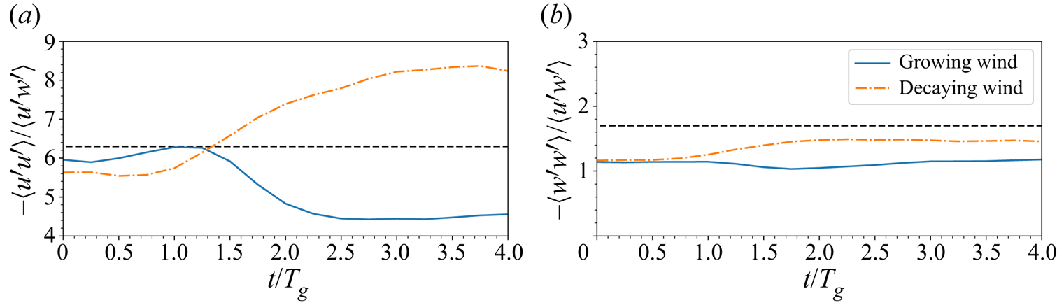
Figure 10. Time variations of the ratio of the turbulent normal stress to the turbulent shear stress at height  $z=0.036\lambda$ in case CU8. Also plotted are the values corresponding to an equilibrium boundary layer over a wave (Belcher & Hunt Reference Belcher and Hunt1993):
  $-\langle u'^{2}\rangle /\langle u'w'\rangle =6.3$ and
 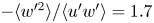 $-\langle w'^{2}\rangle /\langle u'w'\rangle =1.7$, denoted by the black dashed line.
Figure 11. Wave-coherent streamwise velocity and its phase angle relative to the surface elevation for the growing wind in (a,b) case CU8, (c,d) case CU19, and (e, f) case CU42. The results are plotted at (a,c,e)  $t=0$ and (b,d, f)
  $t=T_g$. Also listed is the instantaneous wave age
  $c/u_*$. Here,
  $\tilde {u}$ is normalized by
  $u_{*,0}$.

Figure 12. Same as figure 11, but for the vertical wave-coherent velocity  $\tilde {w}$.
3.3. Evolution of wave-coherent motions
This subsection focuses on the transient features of the wave-coherent streamwise velocity  $\tilde {u}$, vertical velocity
  $\tilde {w}$ and pressure
  $\tilde {p}$, which are useful for the quantitative analyses in the following subsections. We first illustrate
  $\tilde {u}$ and
  $\tilde {w}$ for the growing wind cases at the initial steady state
  $t=0$ and the end of the gust
  $t=T_g$, as plotted in figure 11. For all three cases, the contour patterns of the wave-coherent motions under the unsteady wind condition are qualitatively similar to those under the steady wind condition, as long as their wave ages are in the same range. In the small wave age range (
 $c/u_*\sim 10$, see figures 11a,b,d),
  $\tilde {u}$ shows the non-separated sheltering feature, which corresponds to a phase shift of
  ${\rm \pi} /2$ near the wave surface. The distribution of
  $\tilde {u}$ varies drastically with height near the wave surface. Because the wave ages throughout the gust event in case CU8 are in the same range, the contour shapes of
  $\tilde {u}$ are qualitatively unchanged during the gust despite a significant increase in its magnitude (comparing figures 11a,b). In case CU19, the wave-coherent motions at
  $t=0$ decrease rapidly with height, and overall their magnitudes are relatively small in most of the domain. For the wave age in this case, the gust event has a profound effect on both the magnitude and the contour pattern of the wave-coherent motions. Most notably, the contours of
  $\tilde {u}$ near the wave surface are tilted towards the
  $-x$ direction at
  $t=0$, and the
  $+x$ direction at
  $t=T_g$ (figures 11c,d). In the intermediate wave age, i.e.
  $c/u_*\sim O(20)$, the contour patterns correspond to a phase shift of
  $2{\rm \pi}$ with the height from
  $z=0$ to
  $z=0.05\lambda$ (see figures 11c, f). Note that the discontinuity near
  $z=0.01\lambda \unicode{x2013}0.02\lambda$ is due to the definition of the phase angle, which limits
  $\phi _{\tilde {u}}$ between
  $-{\rm \pi}$ and
  ${\rm \pi}$. For the fast propagating wave at
  $t=0$ in case CU42 (see figure 11e),
  $\tilde {u}$ is nearly symmetric with respect to the wave surface except for a thin layer near the wave surface (for a similar pattern, see Cao & Shen Reference Cao and Shen2021).
The distributions of  $\tilde {w}$ in the growing wind are plotted in figure 12. Compared with the streamwise velocity
  $\tilde {u}$ with complex contour patterns,
  $\tilde {w}$ exhibits relatively simple spatial distributions. Regardless of the wave age and the time instant, the imaginary part of
  $\tilde {w}$ always dominates, i.e.
  $\phi _{\tilde {w}}\approx \pm {\rm \pi}/2$ in the entire domain. When the wave age is not large (figures 12a,b,d),
  $\phi _{\tilde {w}}$ changes from
  $-{\rm \pi} /2$ to
  ${\rm \pi} /2$, while for the relatively large wave ages in figures 12(c,e, f),
  $\phi _{\tilde {w}}$ has a constant value close to
  $-{\rm \pi} /2$ in the region
  $z<0.1\lambda$. This feature of
  $\tilde {w}$ agrees with the Miles (Reference Miles1957) theory based on the Rayleigh equation, which predicts the phase change across the critical layer. A brief review of the critical layer at the steady state can be found in Appendix C.
The evolution of the amplitudes of the wave-coherent motions in the growing wind is shown in figure 13. The vertical coordinates for  $|\tilde {u}|$ and
  $|\tilde {w}|$ are plotted on a logarithmic scale to highlight the near-surface structures. In case CU8,
  $|\tilde {u}|$ and
  $|\tilde {w}|$ reach their peak values around
  $\zeta \sim O(10^{-2})\lambda$. In case CU42,
  $|\tilde {u}|$ and
  $|\tilde {w}|$ decrease nearly monotonically with the height except for
  $|\tilde {u}|$ at early times. In case CU19, the vertical distribution of the wave-coherent velocity amplitudes sees a transition from a monotonic function of height to a more complex pattern during the gust. The pressure amplitudes
  $|\tilde {p}|$ on the logarithmic scale are nearly straight lines with the same slope in most cases, following an
  $\exp (-k\zeta )$ decay with the height, especially when
  $\zeta$ is large. The only exceptions occur at
  $t=0$ in case CU19 and
  $t=T_g$ in case CU42, where
  $|\tilde {p}|$ is prominent only at the wave surface. Away from the surface, the values of
  $|\tilde {p}|$ are too small and may be subject to fluctuations in the triple decomposition statistics. The velocity amplitudes show a similar exponential decay above
  $\zeta \sim O(10^{-2})\lambda$. The exponential decay of the wave-coherent motions is a well-known feature of the asymptotic inviscid solutions at large
  $z$ (Belcher & Hunt Reference Belcher and Hunt1993). In contrast, a noticeable deviation from
  $\exp (-k\zeta )$ may be observed in the distribution of the pressure amplitude near the wave surface because of the wave geometry and the strong gradient in the vertical velocity, as suggested by previous studies (e.g. Yang & Shen Reference Yang and Shen2010; Grare et al. Reference Grare, Peirson, Branger, Walker, Giovanangeli and Makin2013). As the mean velocity increases rapidly during the gust, the viscous effect is enhanced mostly in the thin region near the wave surface, as shown in figure 3. But the outer region remains approximately inviscid, and as a result, the exponential decay still holds there.

Figure 13. Vertical distributions of the amplitudes of the wave-coherent motions  $\tilde {u}$,
  $\tilde {w}$ and
  $\tilde {p}$ for the growing wind in (a–c) case CU8, (d–f) case CU19, and (g–i) case CU42. The exponential decay
  $\exp (-k\zeta )$ is denoted by the black dashed lines. The results are plotted at
  $t/T_g=0, 0.5, 1.0$. All terms are normalized using the wall unit at
  $t=0$.
To identify the wave boundary layer, we plot separately the profiles of the turbulent and wave-coherent parts of the Reynolds shear stress (figure 14). The sign of  $-\langle \tilde {u}\tilde {w}\rangle$ depends on the instantaneous wave age. For slow waves in case CU8 (figures 14a,d), the wave-coherent stress has an opposite sign to the turbulent part, which agrees with the findings of Hara & Sullivan (Reference Hara and Sullivan2015). For fast waves in case CU42 (figures 14c, f), their signs are the same. The transition between these two patterns occurs at the wave age
  $c/u_*\sim 20$, as indicated by the results in case CU19 (figures 14b,e). When
  $-\langle \tilde {u}\tilde {w}\rangle$ is sufficiently large compared with
  $-\langle u'w'\rangle$ (figures 14c,d), the wave boundary layer is most distinguishable, with thickness
  $0.008\lambda \unicode{x2013}0.02\lambda$ (see also the tank experiment by Buckley & Veron Reference Buckley and Veron2016).

Figure 14. Turbulent and wave-coherent parts of the Reynolds shear stress for the growing wind at (a–c)  $t=0$ and (d–f)
  $t=T_g$. All terms are normalized using the wall unit at
  $t=0$. The instantaneous wave ages for (a–f) are
  $c/u_*=8.3$,
  $19.2$,
  $41.6$,
  $4.5$,
  $10.4$,
  $22.3$, respectively.
To summarize, the wave-coherent motions can be identified clearly throughout our simulations, which justifies the use of the triple decomposition in the transient wind–wave process. Owing to page limits for the paper, the time series of the two-dimensional distributions of all wave-coherent components in both growing wind and decaying wind are depicted in the supplementary movies available at https://doi.org/10.1017/jfm.2022.577. A key feature that we see from figures 11–13 is that while the turbulent stresses exhibit the memory effect associated with the gust events (§ 3.2), the wave-coherent motions have a quasi-stationary response to the wind gust and they are strongly dependent on the instantaneous wave age. Furthermore, the growing wind gust has a counterintuitive phenomenon in case CU42: the wave-coherent motions are suppressed, i.e. their magnitudes at  $t=T_g$ (figures 11fand 12f) are smaller than their values at
  $t=0$ (figures 11e and 12e), while in a decaying wind their amplitudes increase. This phenomenon is explained in the following analysis based on the momentum equation.
3.4. Analysis of the wave-coherent momentum equation
To understand further the mechanisms that govern the evolution of the wave-coherent motions during wind gust, we perform more detailed analyses by resorting to the momentum equation. While an energy budget equation for the wave-coherent motions can also be derived in a way similar to the TKE equation (3.1), the phases of the source terms would be complicated because of the product of trigonometric functions. The momentum equation, on the other hand, has a simpler form and preserves directly the phases of the wave-coherent motions. By performing the triple decomposition, the vertical wave-coherent momentum equation can be written as
 \begin{equation} \frac{\partial\tilde{w}}{\partial t}=\underbrace{-(U-c)\,\frac{\partial\tilde{w}} {\partial \xi}}_{\mathcal{A}} -\underbrace{\frac{\partial\widetilde{u'w'}}{\partial \xi}}_{\mathcal{T}} -\underbrace{\frac{1}{\rho}\,\frac{\partial \tilde{p}}{\partial \zeta}}_{\mathcal{P}} +\underbrace{\nu\,\nabla^{2}\tilde{w}}_{\mathcal{V}}, \end{equation}
where  $\mathcal {A}$,
  $\mathcal {T}$,
  $\mathcal {P}$ and
  $\mathcal {V}$ denote the effects of advection, turbulence, pressure gradient and viscosity, respectively. The effect of the wave-coherent stresses
  $\tilde {u}_i\tilde {u}_j$ (
 $i,j=1,3$) is omitted because they have a direct impact on the second harmonic wavenumber
  $4{\rm \pi} /\lambda$ instead of the primary wavenumber
  $2{\rm \pi} /\lambda$, and thus have little effect on the evolution of
  $\tilde {w}$. Apparently, the advection term
  $\mathcal {A}$ and the pressure gradient term
  $\mathcal {P}$ have rapid responses to the wind gust because they are determined by the mean velocity and the wave-coherent motions. The turbulence term
  $\mathcal {T}$, on the other hand, shares a similar memory effect with
  $\widetilde {u'w'}$.
Similar to the decomposition of the wave-coherent motions shown in (2.6), the real part and the imaginary part of each term in the vertical momentum equation (3.4) can be calculated. Figure 15 shows the results for the real parts at  $t=0.5T_g$. Note that the viscous term is found to be negligibly small and has been omitted. In all three cases, the pressure gradient and the advection terms are significant in balancing the real part of (3.4). The turbulence effect nearly vanishes in case CU42. For cases CU8 and CU19, the effect of the turbulence term
  $\mathrm {Re}[\mathcal {T}]$ is relatively strong in the decaying wind, while in the growing wind it is relatively weak. This phenomenon is similar to the time variation of the turbulence intensity discussed in § 3.1, and is also associated with the memory effect of the turbulent stress, which leads to a phase lag in
  $\mathrm {Re}[\mathcal {T}]$ with respect to the rapidly varying
  $\mathrm {Re}[\mathcal {A}]$ and
  $\mathrm {Re}[\mathcal {P}]$. The temporal growth rate
  $\mathrm {Re}[\partial \tilde {w}/\partial t]$ is negligibly small in all cases, suggesting that the real parts are largely balanced regardless of the gust event.
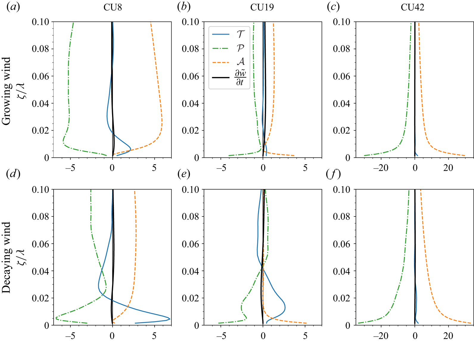
Figure 15. Real part of the terms in the vertical wave-coherent momentum equation for (a–c) the growing wind and (d–f) the decaying wind, at  $t=0.5T_g$. The instantaneous wave ages are
  $c/u_*=5.1, 11.7, 25.2, 7.1, 16.6, 35.2$ in (a–f), respectively. All terms are normalized by
  $ku_{*,0}^{2}$.
In contrast to the relatively simple distributions of the real parts of the terms in (3.4), the distributions of the imaginary parts are more complex, as shown in figure 16. The imaginary part of the viscous term, compared with its real part, is important in the vertical momentum equation near the wave surface, because 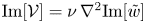 $\mathrm {Im}[\mathcal {V}]=\nu \,\nabla ^{2}\mathrm {Im}[\tilde {w}]$, and
  $\mathrm {Im}[\tilde {w}]$ dominates over
  $\mathrm {Re}[\tilde {w}]$ (figure 12). In general, for the imaginary part, the values of different terms in (3.4) are of the same order, especially in case CU8. Unlike
  $\mathrm {Re}[\partial \tilde {w}/\partial t]$, which is close to zero,
  $\mathrm {Im}[\partial \tilde {w}/\partial t]$ becomes positive in the growing wind and negative in the decaying wind. Hence
  $\mathrm {Im}[\partial \tilde {w}/\partial t]$ is the main contributor to the contour pattern changes presented in figure 12. In particular, for the growing wind in case CU42,
  $\mathrm {Im}[\tilde {w}]$ at
  $t=0$ is negative, noticing that
  $\mathrm {Im}[\tilde {w}]=|\tilde {w}|\sin \phi _{\tilde {w}}<0$ when
  $\phi _{\tilde {w}}\approx -{\rm \pi} /2$ (see figure 12e). The positive
  $\partial \mathrm {Im}[\tilde {w}]/\partial t$ then causes a magnitude reduction in
  $\mathrm {Im}[\tilde {w}]$ during the growing wind event, which is confirmed in figures 12(e, f).

Figure 16. Same as figure 15, but for the imaginary parts.
While the time variation in  $\tilde {w}$ is dominated by
  $\mathrm {Im}[\partial \tilde {w}/\partial t]$, the real and imaginary parts of the momentum equation (3.4) are not independent of each other but dynamically coupled through the differential operator
  $\partial /\partial \xi$. For the advection term and the turbulence term, we have
 $$\begin{gather} \mathrm{Re}[\mathcal{A}]=k(U-c)\,\mathrm{Im}[\tilde{w}], \end{gather}$$
 $$\begin{gather}\mathrm{Im}[\mathcal{A}]={-}k(U-c)\,\mathrm{Re}[\tilde{w}], \end{gather}$$
 $$\begin{gather}\mathrm{Re}[\mathcal{T}]= k\,\mathrm{Im}[\widetilde{u'w'}], \end{gather}$$
 $$\begin{gather}\mathrm{Im}[\mathcal{T}]={-} k\,\mathrm{Re}[\widetilde{u'w'}]. \end{gather}$$
In case CU42, for instance,  $\mathrm {Re}[\mathcal {A}]$ (figures 15c, f) is much larger than
  $\mathrm {Im}[\mathcal {A}]$ (figures 16c, f) because the wave-coherent vertical velocity is dominated by the out-of-phase imaginary part
  $\mathrm {Im}[\tilde {w}]$ (see figure 12).
Next, we perform a quantitative analysis of the wave-coherent motions by utilizing and comparing with the viscous curvilinear model proposed by Cao et al. (Reference Cao, Deng and Shen2020). The model originates from the triple decomposition of the Navier–Stokes equations for wind turbulence over a monochromatic wave under the steady wind–wave condition. In their derivation, the nonlinear terms associated with the turbulent stress and the second-order terms of  $O((ka)^{2})$ related to the grid transformation are neglected. The governing equation for the vertical wave-coherent velocity
  $\tilde {w}$ reads
 \begin{align} &\displaystyle {-\frac{\nu}{ik}}\left(\frac{\mathrm{d}^{4}}{\mathrm{d}\zeta^{4}} -2k^{2}\,\frac{\mathrm{d}^{2}}{\mathrm{d}\zeta^{2}}+k^{4}\right)\mathcal{F}[\tilde{w}] +\left[(U-c)\left(\frac{\mathrm{d}^{2}}{\mathrm{d}\zeta^{2}}-k^{2}\right) -\frac{\mathrm{d}^{2}U}{\mathrm{d}\zeta^{2}}\right]\mathcal{F}[\tilde{w}] \nonumber\\ &\quad \displaystyle =\mathcal{F}\left[\frac{\partial }{\partial t}\left(\frac{\partial\tilde{u}}{\partial\zeta}-\frac{\partial\tilde{w}}{\partial\xi}\right)\right] +\nu\,\mathcal{F}[\eta]\,\frac{\mathrm{d}^{2}}{\mathrm{d}\zeta^{2}} \left[\left(\frac{\zeta}{h}-1\right)\frac{\mathrm{d}^{2}U}{\mathrm{d}\zeta^{2}}\right], \end{align}
where  $\mathcal {F}$ denotes the Fourier transform operator. For completeness, we keep the time derivative term that was neglected by Cao et al. (Reference Cao, Deng and Shen2020). But its actual value is also found to be insignificant compared with the other terms in the present wind gust cases. The mean profile
  $U(\zeta )$ is provided by the simulation, and the boundary conditions are
 $$\begin{gather} \tilde{w}(\zeta=0)=w_s,\quad \tilde{w}(\zeta\rightarrow\infty)=0, \end{gather}$$
 $$\begin{gather}\left.\frac{\mathrm{d}\tilde{w}}{\mathrm{d}\zeta}\right|_{\zeta=0} ={-}\frac{\mathrm{d}u_s}{\mathrm{d}\xi}+\frac{\mathrm{d}U}{\mathrm{d}\zeta}\,\frac{\mathrm{d}\eta}{\mathrm{d}\xi},\quad \left.\frac{\mathrm{d}\tilde{w}}{\mathrm{d}\zeta}\right|_{\zeta\rightarrow\infty}=0, \end{gather}$$
where  $u_s$ and
  $w_s$ are the streamwise and vertical wave orbital velocities, respectively (see Appendix A).
Here, the Dirichlet boundary condition for  $\tilde {w}$ at
  $\zeta =0$ is prescribed by the wave orbital velocity, and its derivative
  ${\mathrm {d}\tilde {w}}/{\mathrm {d}\zeta }$ is obtained from the continuity equation. In practice, the top boundary condition (
 $\zeta \rightarrow \infty$) can be evaluated at a height where the magnitude of
  $\tilde {w}$ is sufficiently small, say
  $\zeta =0.5\lambda$ (Cao et al. Reference Cao, Deng and Shen2020). Near the wave surface, the imaginary part of the vertical wave-coherent velocity dominates over the real part because of the
  ${\rm \pi} /2$ phase difference between the vertical wave orbital velocity and the surface elevation (see (A6)).
In figure 17, we present  $\mathrm {Im}[\tilde {w}]$ at three instants in the growing wind gust. The evolution of
  $\mathrm {Im}[\tilde {w}]$ dominates the qualitative features shown in figure 12. For example, the phase change of
  ${\rm \pi}$ in the vicinity of the wave surface in case CU8 (figure 12a) corresponds to the sign reversal at small
  $\zeta /\lambda$ in figure 17(a). Consistent with the positive
  $\partial \mathrm {Im}[\tilde {w}]/\partial t$ shown in figure 17,
  $\mathrm {Im}[\tilde {w}]$ increases with the growing wind in all cases (figure 12). In general, the LES result agrees well quantitatively with the model prediction at both the steady state (
 $t=0$) and the non-equilibrium state (
 $t=0.5T_g$ and
  $t=T_g$). Hence the quasi-linear mechanism (Cao et al. Reference Cao, Deng and Shen2020) that governs the response of
  $\mathrm {Im}[\tilde {w}]$ to the mean velocity profile
  $U$ is effective even under the gusty condition.

Figure 17. Imaginary part of the vertical wave-coherent velocity for the growing wind in (a) case CU8, (b) case CU19, and (c) case CU42. Also plotted are the corresponding results computed from the viscous curvilinear model, denoted by the black solid lines.
For  $\mathrm {Re}[\tilde {w}]$, on the other hand, the difference between the model prediction and the LES result is noticeable. In figure 18, we plot the instantaneous result at
  $t=0.5T_g$ as an example. Qualitatively, the result predicted by the model has a shape similar to the LES result, in which
  $\mathrm {Re}[\tilde {w}]$ first increases with the height and then decreases after reaching a positive peak value. The modelling of
  $\mathrm {Re}[\tilde {w}]$ is challenging because it has a small magnitude compared with
  $\mathrm {Im}[\tilde {w}]$. At
  $t=0.5T_g$, the peak value of
  $\mathrm {Re}[\tilde {w}]$ is approximately one-fifth of the corresponding value of
  $\mathrm {Im}[\tilde {w}]$ in case CU8 (comparing figures 17a and 18a). At larger wave ages in case CU42, the difference between the magnitudes of
  $\mathrm {Im}[\tilde {w}]$ and
  $\mathrm {Re}[\tilde {w}]$ can be as large as two orders of magnitude (figures 17c and 18c). The viscous curvilinear model fails to predict the weak
  $\mathrm {Re}[\tilde {w}]$ because the impacts of the turbulence and second-order terms omitted in the derivation of the model are no longer negligible.

Figure 18. Real part of the vertical wave-coherent velocity for the growing wind in (a) case CU8, (b) case CU19, and (c) case CU42. The results computed from the viscous curvilinear model are denoted by the black solid lines.
From the analyses in this subsection, we obtain a clear picture of the wave-coherent motions. First, compared with the turbulent stress, the wave-coherent motions respond instantly to the gust event and show strong dependency on the wave age. Besides, the gust event leads to a drastic change in the out-of-phase component  $\mathrm {Im}[\tilde {w}]$, and has little impact on the in-phase component
  $\mathrm {Re}[\tilde {w}]$. In the next subsection, we investigate whether these phenomena are responsible for producing the drag hysteresis that has been observed in laboratory and field experiments (Waseda et al. Reference Waseda, Toba and Tulin2001; Hwang et al. Reference Hwang, García Nava and Ocampo-Torres2011) and how the change in
  $\mathrm {Im}[\tilde {w}]$ contributes to the variation in wind–wave energy transfer.
3.5. Wind gust impact on wave growth
It is well recognized that the wave-coherent motions play a critical role in the wind–wave momentum and energy transfer. In this subsection, we investigate how their time variations affect these processes. We first examine the evolution of the form drag  $\tau _p$ and viscous drag
  $\tau _{\nu }$. In the present study, we use the sign convention such that the drags are positive when the direction of the momentum flux is from the wind to the wave, such as at small wave ages. As shown in figure 19, the viscous drag
  $\tau _{\nu }$ changes continuously during the gust and remains positive. In all cases,
  $\tau _{\nu }$ at the end of the growing wind gust is slightly larger than that at the start of the decaying wind gust, while at the end of the decaying gust,
  $\tau _{\nu }$ nearly vanishes and is significantly smaller than its initial value in a growing wind. This hysteresis effect exhibited by
  $\tau _{\nu }$ is associated primarily with the evolution of the mean velocity profile and the mean shear. As discussed in § 3.1, the uniform change in the mean velocity caused by the external force occurs mainly in the outer region where the mean shear is expected to be roughly unchanged during the gust. The near-wall region is dominated by viscosity such that the mean velocity and its gradient are affected by their past states.

Figure 19. Evolution of form drag and viscous drag during the wind gust ( $0< t< T_g$). The start (
 $t=0$) and end (
 $t=T_g$) of the gust are denoted by dash marks (–) and circles, respectively, and the arrows denote the direction of time increase.
The form drag  $\tau _p$ sees an abrupt change at the start and end of the gust. During the wind gust, the variations in
  $\tau _p$ are relatively small at first, and this feature is shared in all cases. Near the end of the gust, there is a substantial change in
  $\tau _p$ for cases CU8 and CU19, while in case CU42 the change in
  $\tau _p$ is trivial. To understand the behaviours of
  $\tau _p$, we consider its definition:
 \begin{equation} \tau_p=\frac{1}{L_x}\int_0^{L_x}\frac{p\eta_x}{\rho}\,\mathrm{d}x =\frac{ka\left.\mathrm{Im}[\tilde{p}]\right|_{\zeta=0}}{\rho}. \end{equation}
The pressure at the wave surface can be obtained by integrating the imaginary part of the vertical momentum equation (3.4). Keeping only the dominant terms, we can rewrite (3.12) as
 \begin{equation} \tau_p=ka\int_0^{\lambda} k(U-c)\,\mathrm{Re}[\tilde{w}]\,\mathrm{d}\zeta +ka\int_0^{\lambda}\frac{\partial}{\partial t}\mathrm{Im}[\tilde{w}]\,\mathrm{d}\zeta. \end{equation}
The contribution to the form drag is then decomposed into two parts, the advection of  $\mathrm {Re}[\tilde {w}]$ and the time variation of
  $\mathrm {Im}[\tilde {w}]$ caused by the wind gust. For a wind turbulence field at the steady state, only the advection term needs to be included in the calculation, while the gustiness term reduces to zero (see e.g. Cao et al. Reference Cao, Deng and Shen2020).
When the wind is unsteady, the gustiness term becomes important. In figure 20, we plot the time-averaged contributions from the advection and gustiness terms to the form drag during  $0< t< T_g$. For the advection term, the contribution varies with the wave age, which determines the advection velocity
  $U-c$. For the contribution by the gustiness, however, the wave age has less influence because the magnitudes of
  $\partial \mathrm {Im}[\tilde {w}]/\partial t$ are comparable in different cases (see figure 16). Figure 20 shows that in all cases, the gustiness term is comparable to (cases CU8 and CU19) or stronger than (case CU42) the advection term. Therefore, the out-of-phase component
  $\mathrm {Im}[\tilde {w}]$ that changes rapidly during the gust plays an at least equally important role as the in-phase component
  $\mathrm {Re}[\tilde {w}]$ in the wind–wave momentum transfer.
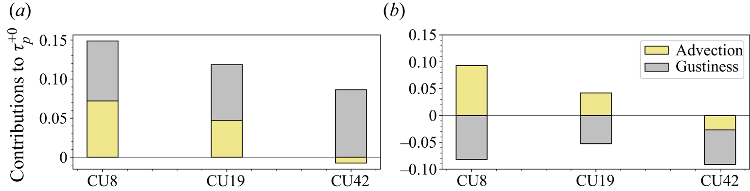
Figure 20. Contributions of the advection and gustiness terms to the form drag in (a) the growing wind and (b) the decaying wind. All terms are calculated by taking the time average during  $0< t< T_g$.
We now revisit figure 19 to explain the behaviour of  $\tau _p$ based on the decomposition (3.13). The abrupt change immediately after
  $t=0$ and before
  $t=T_g$ is caused by the contribution of the gustiness term. During
  $0< t< T_g$, cases CU8 and CU19 have a noticeable change in
  $\tau _p$ because the advection term itself is changing with the mean velocity, and its contribution is comparable to that of the gustiness term (figure 20). For case CU42, although the mean velocity and the advection term change substantially during the wind gust, the magnitude of the advection term is much smaller than that of the gustiness term, as shown in figure 20. Therefore, the value of
  $\tau _p$ is relatively invariant during this process.
To quantify the amount of wind energy transferred to wave, we calculate the wave growth rate  $\beta$ (Miles Reference Miles1957) and the temporal energy growth rate
  $\gamma$ (Donelan & Pierson Reference Donelan and Pierson1987):
 $$\begin{gather} \beta=\frac{2\tau_p}{(aku_*)^{2}}, \end{gather}$$
 $$\begin{gather}\gamma=\left(\frac{u_*}{c}\right)^{2}\beta=\frac{2\tau_p}{(akc)^{2}}. \end{gather}$$
 In table 3, we list the time-averaged results of  $\beta$ and
  $\gamma$ during the wind gust (
 $0< t< T_g$). We follow Miles & Ierley (Reference Miles and Ierley1998) to obtain
  $\bar {\beta }$ by calculating separately the mean form drag and the average of the square of the friction velocity, and then using them to calculate
  $\bar {\beta }$. For both
  $\bar {\beta }$ and
  $\bar {\gamma }$, there is a distinct difference between the growing wind result and the decaying wind result. The primary reason for this difference is due to the hysteresis phenomenon in the variation of the form drag and the viscous drag (figure 19).
Table 3. Time-averaged  $\beta$ and
  $\gamma$ during
  $0< t< T_g$. Here,
  $\overline {(\ )}$ is the time-averaging operator. Also listed is the strength of the gust event
  $|\Delta U/U|/\omega T_g$, where
  $\Delta U/U=[U(0.02\lambda,T_g)-U(0.02\lambda,0)]/U(0.02\lambda,0.5T_g)$ is the relative change in the mean profile, and
  $\omega$ is the wave frequency.

We plot  $\beta$ as a function of the wave age
  $c/u_*$ in figure 21(a). The results denoted by the light grey and dark grey symbols are instantaneous values at
  $t=0$, while those during the gust, denoted by coloured symbols, are calculated as the time-averaged values (see table 3). At the steady state before the gust event occurs,
  $\beta$ varies with the wave age and is in general consistent with the results in the literature (Sullivan et al. Reference Sullivan, Mcwilliams and Moeng2000; Kihara et al. Reference Kihara, Hanazaki, Mizuya and Ueda2007; Yang & Shen Reference Yang and Shen2010; Druzhinin et al. Reference Druzhinin, Troitskaya and Zilitinkevich2012; Åkervik & Vartdal Reference Åkervik and Vartdal2019). When the wind gust starts, there is an immediate change in the wave age associated with the time-varying friction velocity
  $u_*$ (see the evolution of the friction drag in figure 19). The shift in the wave age has been incorporated into the wind input source terms in phase-averaged wave models to account for the gustiness effect on the wave energy growth (Janssen Reference Janssen2004). For atmospheric variability with a time scale much larger than the wave period and the wind turbulence in a quasi-equilibrium state, this simple approximation is likely appropriate. But more generally, especially for a rapidly changing wind field, this is not the case. Our result in figure 21(a) shows a noticeable deviation of
  $\bar {\beta }$ from the steady state value. The strength of the wind gust can be measured roughly by
  $|\Delta U/U|/\omega T_g$ (table 3), or, more generally,
  $(\partial U/\partial t)/\omega |U|$ (see Miles & Ierley Reference Miles and Ierley1998). Note that while by this definition the wind gust event is the weakest in the high wave age case CU42, the deviation of
  $\beta$ from the steady-state values is most significant in this case because the gustiness effect has the largest relative contribution to the form drag (see figure 20).
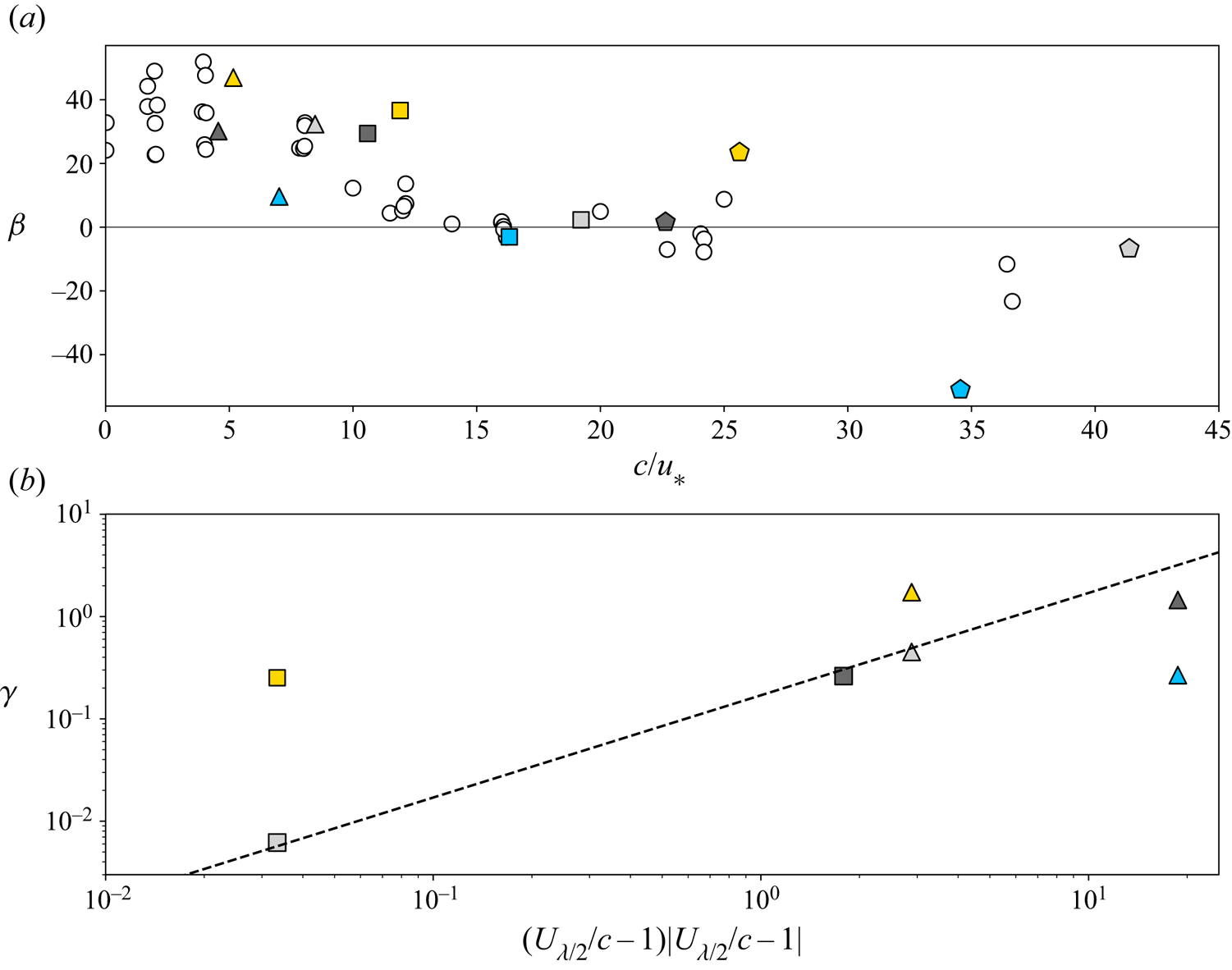
Figure 21. (a) Wave growth rate  $\beta$ scaled with the friction velocity
  $u_*$. (b) Temporal growth rate
  $\gamma$ scaled with the mean wind velocity at the height of half-wavelength
  $U_{\lambda /2}$. In (a), the results in cases CU8, CU19 and CU42 are denoted by triangles, squares and pentagons, respectively. The symbols with the filled colours light grey and dark grey denote the initial steady-state results, and those with the colours gold and blue are the time-averaged values
  $\bar {\beta }$ during the growing wind and the decaying gust, respectively. Also plotted are the steady-state results with similar wave steepness (
 $ak<0.1$) obtained using direct numerical simulation (Sullivan et al. Reference Sullivan, Mcwilliams and Moeng2000; Kihara et al. Reference Kihara, Hanazaki, Mizuya and Ueda2007; Yang & Shen Reference Yang and Shen2010; Druzhinin et al. Reference Druzhinin, Troitskaya and Zilitinkevich2012) and LES (Åkervik & Vartdal Reference Åkervik and Vartdal2019), denoted by circles. In (b), only those results with positive values of
  $\gamma$ and
  $U_{\lambda /2}/c-1$ are plotted. The black dashed line denotes the parametrization proposed by Donelan et al. (Reference Donelan, Babanin, Young and Banner2006):
  $\gamma =0.17(U_{\lambda /2}/c-1)|U_{\lambda /2}/c-1|$.
In figure 21(b), we plot  $\gamma$ using an alternative scaling based on
  $U_{\lambda /2}$, the characteristic mean velocity at
  $\zeta =\lambda /2$ (Donelan et al. Reference Donelan, Babanin, Young and Banner2006). The steady-state values are consistent with the parametrization proposed by Donelan et al. (Reference Donelan, Babanin, Young and Banner2006),
  $\gamma =0.17$. While this parametrization is effective in reducing the scattering compared with the scaling based on
  $u_*$ shown in figure 21(a), it underestimates
  $\gamma$ in the growing wind and overestimates
  $\gamma$ in the decaying wind. The deviation, which can be up to several orders of magnitude, is a consequence of the change in the mean velocity
  $U_{\lambda /2}$ and
  $\gamma$ itself. Therefore, the non-stationary effect associated with the wind gust cannot be incorporated into such parametrized wind input models by simply using a shift in the wave age
  $c/U_{\lambda /2}$. More research on the model development, which is beyond the scope of this work, is called for in future studies.
4. Concluding remarks
In this study, we have performed high-resolution wall-resolved LES of wind turbulence over a travelling wave, where the wind field is subject to an impulsive growing and decaying gust event. Multiple wave speeds are designed to cover representative wave ages. Compared with the vast majority of current research that assumes a stationary or quasi-stationary state for the wind–wave interaction, we investigate the non-stationary state of wind turbulence, which exists widely in the atmospheric boundary layer above ocean waves. This study focuses on the transient features of the turbulent and wave-coherent motions as well as their impact on the momentum and energy transfer.
We show that the turbulence fluctuations have a delayed response to the mean shear, similar to classical channel flow results. We find that this memory effect is caused mainly by the phase delay in the production induced by the mean shear, the pressure–strain correlation and the dissipation. On the other hand, the wave-coherent motions and the associated production are found to have a quasi-stationary response to the gust: the qualitative features of the wave-coherent motions during the wind gust are similar to those in a steady wind turbulence with the same instantaneous wave age. By evaluating the terms in the wave-coherent vertical momentum equation, we find that the component of the vertical wave-coherent velocity  $\tilde {w}$ out of phase with the surface elevation,
  $\mathrm {Im}[\tilde {w}]$, dominates the change in
  $\tilde {w}$, while the in-phase component,
  $\mathrm {Re}[\tilde {w}]$, has a much smaller temporal growth rate. We show that as a result of the quasi-stationary response,
  $\mathrm {Im}[\tilde {w}]$ can be predicted by the viscous curvilinear model developed originally for steady state, even during the wind gust event, while
  $\mathrm {Re}[\tilde {w}]$ cannot be predicted, owing to the relatively small amplitude.
We have also investigated the effect of wind gust on wind–wave momentum and energy transfer. The evolution of the form drag and the viscous drag demonstrates a hysteresis phenomenon and presents a distinct difference between the growing and decaying wind. We have identified  $\partial {\mathrm {Im}[\tilde {w}]}/\partial t$ as a key contributor to the form drag (and thus the wave growth) during wind gust. Our result also shows that this contribution from the out-of-phase component
  $\mathrm {Im}[\tilde {w}]$ is comparable to that caused by the advection of the in-phase component
  $\mathrm {Re}[\tilde {w}]$ at low and intermediate wave ages, and much stronger at a high wave age.
A major implication of the discovery of the transient behaviours of turbulence in wind gust is associated with the closure model of the Reynolds stress. The local turbulence equilibrium assumption used in the classical wind–wave growth theories is no longer valid. Therefore, the wind gustiness effect poses significant challenges to the modelling of the non-equilibrium turbulent stresses, for which more research is needed. From a more practical perspective, our discovery shows the necessity to incorporate the transient features of the wind field into the wind input models in operational wave models. Such improvement may also be helpful in reducing the large scattering found in the wave growth rate from field observations, which is plotted against the wave age alone, typically, but without considering the transient effect. Finally, we remark that the simulation set-up in the present study is relatively simple, limited by the computational cost needed for resolving the viscous sublayer and performing the ensemble runs. More realistic marine conditions, such as irregular waves and dynamical coupling between wind and waves, should be taken into consideration in future studies.
Supplementary movies
Supplementary movies are available at https://doi.org/10.1017/jfm.2022.577.
Acknowledgements
The authors gratefully acknowledge the referees for their constructive and valuable comments.
Funding
This work is supported by the Office of Naval Research.
Declaration of interests
The authors report no conflict of interest.
Appendix A. Wind turbulence solver
The numerical solver developed originally by Yang & Shen (Reference Yang and Shen2011a,Reference Yang and Shenb) has been used extensively and validated in studies on wind–wave interaction (e.g. Yang et al. Reference Yang, Meneveau and Shen2013; Hao & Shen Reference Hao and Shen2019; Cao et al. Reference Cao, Deng and Shen2020; Cao & Shen Reference Cao and Shen2021). The filtered Navier–Stokes equations (2.1) and (2.2) are transformed from the physical domain into the computational domain by
 \begin{equation} \tau=t,\quad \xi=x,\quad \psi=y,\quad \zeta=\frac{z-\eta(x,y,t)}{h-\eta(x,y,t)}\,h, \end{equation}
where  $\xi$,
  $\psi$,
  $\zeta$ and
  $\tau$ are respectively the space and time coordinates in the computational domain, and
  $h=L_z$ is the mean domain height. The Jacobian matrix corresponding to the transformation (A 1) is
 \begin{equation} \boldsymbol{J} = \left[ \begin{array}{ccc} \displaystyle \dfrac{\partial \xi}{\partial x} & \displaystyle \dfrac{\partial \xi}{\partial y} & \displaystyle\dfrac{\partial \xi}{\partial z} \\[6pt] \displaystyle \dfrac{\partial \psi}{\partial x} & \displaystyle\dfrac{\partial \psi}{\partial y} & \displaystyle \dfrac{\partial \psi}{\partial z} \\[6pt] \displaystyle \dfrac{\partial \zeta}{\partial x} & \displaystyle\dfrac{\partial \zeta}{\partial y} & \displaystyle \dfrac{\partial \zeta}{\partial z} \\ \end{array} \right] =\left[\begin{array}{ccc} \displaystyle 1 & \displaystyle 0 & \displaystyle 0 \\[3pt] \displaystyle 0 & \displaystyle 1 & \displaystyle 0 \\[6pt] \displaystyle \dfrac{\zeta-h}{h-\eta}\,\dfrac{\partial \eta}{\partial x} & \displaystyle \dfrac{\zeta-h}{h-\eta}\,\dfrac{\partial \eta}{\partial y} & \displaystyle \dfrac{h}{h-\eta} \\ \end{array} \right]. \end{equation}
Then the governing equations (2.1) and (2.2) become
 \begin{equation} J_{ji}\,\frac{\partial u_i}{\partial \xi_j}=0, \end{equation}
 \begin{align} \frac{\partial u_i}{\partial \tau}+\delta_{j3}\,\frac{\partial \zeta}{\partial t}\,\frac{\partial u_i}{\partial \xi_j}+J_{kj}\,\frac{\partial (u_iu_j)}{\partial \xi_k}&={-}\frac{J_{ji}}{\rho}\,\frac{\partial p}{\partial \xi_j}+J_{kj}\,\frac{\partial\tau_{ij}^{d}}{\partial\xi_k}\nonumber\\ &\quad +\nu J_{nj}\,\frac{\partial}{\partial\xi_n}\left(J_{kj}\,\frac{\partial u_i}{\partial \xi_k}\right)+B(t)\,\delta_{i1}, \end{align}
where the time derivative in the physical space is calculated by
 \begin{equation} \frac{\partial}{\partial t} = \frac{\partial}{\partial \tau} +\frac{\zeta-h} {h-\eta}\,\frac{\partial\eta}{\partial t}. \end{equation}
 In the above equation, the pressure  $p$ is calculated at each time step by solving the Poisson equation, while
  $B(t)$ is prescribed by (2.3). The wave surface boundary conditions are provided by the Airy wave solution (Dean & Dalrymple Reference Dean and Dalrymple1991)
 $$\begin{gather} \eta(x,t) = a\cos(kx-\omega t), \end{gather}$$
 $$\begin{gather}u_s(x,t) = \omega a\cos(kx-\omega t), \end{gather}$$
 $$\begin{gather}w_s(x,t) = \omega a\sin(kx-\omega t), \end{gather}$$
where  $u_s$ and
  $w_s$ are the horizontal and vertical orbital velocities at the wave surface, respectively, and
  $a$ is the wave amplitude. The angular frequency
  $\omega$ and the wavenumber
  $k$ satisfy the dispersion relation for deep water
  $\omega ^{2}=gk$.
Appendix B. Normalized mean wind velocity defect
We examine the initial evolution of the mean profile in the near surface region by using a different scaling of the velocity. Following He & Seddighi (Reference He and Seddighi2013), we define
 \begin{equation} \hat{U}(\zeta,t)=\frac{U(\zeta,t)-U(\zeta,0)}{U(L_z,t)-U(L_z,0)}, \end{equation}
where  $U(L_z,t)$ is the mean velocity at the top boundary of the computational domain. The results are plotted in figure 22. The temporal evolution of the (velocity) boundary layer thickness
  $\delta _{99}$ is similar to a boundary layer developing in space. When the wind gust starts (
 $t\approx 0$), this normalized velocity is constant, i.e.
  $\hat {U}(\zeta >0)=1$, except at the surface, i.e.
  $\hat {U}(\zeta =0)=0$. For laminar flows over a flat plate, the mean profile then yields the solution to the Stokes problem:
  $\hat {U}(\zeta,t)=\mathrm {erf}(\zeta )/\sqrt {\nu t}$, where
  $\mathrm {erf}$ is the error function. For the present flow over a travelling wave, the distribution of
  $\hat {U}(\zeta,t)$ is also similar to the Stokes solution (figure 22) because the viscosity dominates this high-shear region. However, the deviation of the LES result from the Stokes solution is slightly larger than that in a transient channel flow (He & Seddighi Reference He and Seddighi2015) because of the wave geometry and wave orbital velocity.

Figure 22. Evolution of the normalized mean wind velocity profiles  $\hat {U}(\zeta,t)$ defined in (B1) in (a) the growing wind and (b) the decaying wind, in case CU8. The velocity profiles are plotted during
  $2.65< t^{+0}<130$, and the time interval between two consecutive velocity profiles is
  $\Delta t^{+0}=15.9$. Our numerical result and the Stokes problem solution are denoted by the solid lines and dashed lines, respectively. Also plotted is the boundary layer thickness
  $\delta _{99}$, denoted by the black dash-dotted line.
Appendix C. Critical layer at steady state
The critical layer, at which height the mean wind speed equals the wave phase velocity, corresponds to a singular point in the inviscid Rayleigh equation and thus plays a significant role in the Miles (Reference Miles1957) wave-growth mechanism. In case CU8, the critical layer at  $t=0$ is close to the surface (figure 3), in the buffer layer, owing to the small wave age. In case CU42,
  $\zeta _c$ is larger than the computational domain height (not plotted). At such a height
  $\zeta >O(\lambda )$, the wave-coherent motions are much weaker than the turbulence motions (Sullivan & McWilliams Reference Sullivan and McWilliams2010). Therefore, the critical layers in both case CU8 and case CU42 have little dynamic effects on wave growth. On the other hand, in case CU19,
  $\zeta _c$ is sufficiently large that the critical layer is in the logarithmic region, but not too large so that the wave-coherent motions can still be identified at this height. In figure 23, we plot the phase-averaged velocity at the steady state in the wave-following frame for case CU19 to illustrate the qualitative feature of the critical layer. As shown, across the critical layer height
  $\zeta _c$, there is a change in the sign of
  $\langle u\rangle -c$, resulting in the closed loops of the streamlines. This phenomenon, also known as the cat-eye structure (Lighthill Reference Lighthill1962), is consistent with the observations in previous studies (e.g. Sullivan et al. Reference Sullivan, Mcwilliams and Moeng2000; Yang & Shen Reference Yang and Shen2010).

Figure 23. Streamlines of the phase-averaged velocity in the moving frame of reference in case CU19 for growing wind at  $t=0$. The streamwise velocity magnitude is denoted by the contour colour. Also plotted is the critical layer height, denoted by the black dashed line.
Appendix D. Calculation of form drag
Here, we outline the calculation of the form drag in (3.12) and (3.13). Following (2.6), we can rewrite the wave-coherent pressure at the wave surface as
 \begin{equation} \tilde{p}(x,\zeta=0)=\mathrm{Re}[\tilde{p}](\zeta=0)\cos(kx)-\mathrm{Im}[\tilde{p}](\zeta=0)\sin(kx). \end{equation}
 In the moving frame, the surface elevation is fixed,  $\eta (x)=a\cos (kx)$, where
  $a$ is the wave amplitude, thus
  $\eta _x(x)=-ka\sin (kx)$. Substituting this into the definition of the form drag and noting that only the wave-coherent part of pressure can contribute to wave growth, we can obtain
 \begin{align} \tau_p=\frac{1}{L_x}\int_0^{L_x}p\eta_x\, \mathrm{d} x &=\frac{ka}{L_x}\int_0^{L_x}\bigl(\mathrm{Im}[\tilde{p}]\sin^{2}(kx)\nonumber\\ &\quad -\mathrm{Re}[\tilde{p}]\sin(kx)\cos(kx)\bigr)\,\mathrm{d} x. \end{align}
Note that the integral of the second part is zero. Therefore, the calculation of the form drag is simplified to
 \begin{equation} \tau_p=ka\left.\mathrm{Im}[\tilde{p}]\right|_{\zeta=0}. \end{equation}
 The information of  $\mathrm {Im}[\tilde {p}]$ is connected to
  $\tilde {w}$ by taking the imaginary part of the wave-coherent momentum equation (3.4) and rearranging the terms:
 \begin{equation} \frac{1}{\rho}\,\frac{\mathrm{d}\,\mathrm{Im}[\tilde{p}]}{\mathrm{d} \zeta}={-}k(U-c)\,\mathrm{Re}[\tilde{w}] -\frac{\partial\mathrm{Im}[\tilde{w}]}{\partial t}+\mathrm{Im}[\mathcal{T}]+\mathrm{Im}[\mathcal{V}]. \end{equation}
The above equation can be integrated, and after neglecting the higher-order terms, we can obtain
 \begin{equation} \frac{\left.\mathrm{Im}[\tilde{p}]\right|_{\zeta=0}}{\rho}=\int_0^{\lambda}k(U-c)\,\mathrm{Re}[\tilde{w}]\,\mathrm{d}\zeta +\int_0^{\lambda}\frac{\partial\mathrm{Im}[\tilde{w}]}{\partial t}\,\mathrm{d}\zeta. \end{equation}


 Open access