


1. Introduction
Recently, the motion of micro-swimmers in complex fluids has attracted a considerable attention as it is relevant in medicine, ecology and technological applications (Datt et al. Reference Datt, Natale, Hatzikiriakos and Elfring2017; Li, Lauga & Ardekani Reference Li, Lauga and Ardekani2021). Examples of this problem include the locomotion of mammalian spermatozoa in viscoelastic mucus (Katz & Berger Reference Katz and Berger1980), the Lyme disease spirochete Borrelia burgdorferi penetrating the extracellular matrix of mammalian skin (Harman et al. Reference Harman, Dunham-Ems, Caimano, Belperron, Bockenstedt, Fu, Radolf and Wolgemuth2012), bacteria producing extracellular polymeric substances and forming biofilms (Costerton et al. Reference Costerton, Cheng, Geesey, Ladd, Nickel, Dasgupta and Marrie1987). A proper understanding of the micro-swimmer's hydrodynamics in these environments is not only interesting from a scientific perspective, but also plays a significant role in designing efficient swimming devices relevant for drug delivery (Gao & Wang Reference Gao and Wang2014), gene therapy and bionic (Yan et al. Reference Yan, Zhou, Vincent, Deng, Yu, Xu, Xu, Tang, Bian, Wang, Kostarelos and Zhang2017) applications (Li et al. Reference Li, Qin, Gopinath, Arratia, Thomases and Guy2017a).
The complex carrier fluid can significantly affect the swimming behaviour of the individual micro-swimmers. For example, the bacteria Chlamydomonas reinhardtii and E. coli can swim significantly faster in viscoelastic fluids or a polymer solution than in a Newtonian fluid, and E. coli follows straighter trajectories in the polymer solution because of the suppressed wobbling of the cell body (Patteson et al. Reference Patteson, Gopinath, Goulian and Arratia2015; Li et al. Reference Li, Esteban-Fernández de Ávila, Gao, Zhang and & Wang2017b). In contrast, the algal cell C. reinhardtii is hindered in a viscoelastic fluid than in a Newtonian fluid as the viscoelasticity restricts the displacement of the flagella near the cell body (Smith et al. Reference Smith, Gaffney, Gadêlha, Kapur and Kirkman-Brown2009). It is concluded that fluid viscoelasticity affects the swimming ability (both hastens and hinders) of an organism depending on its self-propelling mode (Elfring & Goyal Reference Elfring and Goyal2016), the structural properties of the body (Zhu et al. Reference Zhu, Do-Quang, Lauga and Brandt2011) and the rheological behaviour of the surrounding fluid (Dasgupta et al. Reference Dasgupta, Liu, Fu, Berhanu, Breuer, Powers and Kudrolli2013). A classical ‘squirmer’ is widely employed to investigate the swimming of a micro-swimmer through a viscoelastic and shear-dependent medium. This model was proposed by Lighthill (Reference Lighthill1952) and extended by Blake (Reference Blake1971), and it has been successfully used to mimic the self-propulsion of a swimmer with a dense array of cilia on its surface, such as Opalina and Volvox (Pedley, Brumley & Goldstein Reference Pedley, Brumley and Goldstein2016). The studied scenarios include the self-propelled organisms’ nutrient uptake (Magar, Goto & Pedley Reference Magar, Goto and Pedley2003; Magar & Pedley Reference Magar and Pedley2005), their hydrodynamic interactions with a wall (Ishimoto & Gaffney Reference Ishimoto and Gaffney2013; Ouyang, Lin & Ku Reference Ouyang, Lin and Ku2018a), the two-body hydrodynamic interactions (Ishikawa, Simmonds & Pedley Reference Ishikawa, Simmonds and Pedley2006; Götze & Gompper Reference Götze and Gompper2010; Navarro & Pagonabarraga Reference Navarro and Pagonabarraga2010; Ouyang, Lin & Ku Reference Ouyang, Lin and Ku2019) and their collective swimming dynamics (Ishikawa, Locsei & Pedley Reference Ishikawa, Locsei and Pedley2008; Ishikawa & Pedley, Reference Ishikawa and Pedley2008; Zöttl & Stark Reference Zöttl and Stark2014). Zhu et al. (Reference Zhu, Do-Quang, Lauga and Brandt2011) numerically study the steady locomotion of a neutral squirmer in a Giesekus fluid (a viscoelastic fluid model) at a low Reynolds number, finding that the viscoelasticity leads to a slower speed than in a Newtonian fluid, and a minimum speed occurs at a Weissenberg number of order 1. They also find a higher swimming efficiency in the polymeric fluid than in the Newtonian fluid. This also applies to the pusher and puller, reported in their subsequent study (Zhu, Lauga & Brandt Reference Zhu, Lauga and Brandt2012). Recently, Binagia et al. (Reference Binagia, Phoa, Housiadas and Shaqfeh2020) propose an alternative mechanism for enhancing the speed of a squirmer by coupling the fluid elasticity and local swirling flow induced by the azimuthal term of the squirmer model. This azimuthal term generates no net change of the squirmer's speed in a Newtonian fluid in the Stokes regime (Re = 0), but can significantly affect the speed by altering the flow structure behind the squirmer in a viscoelastic fluid (Binagia et al. Reference Binagia, Phoa, Housiadas and Shaqfeh2020; Housiadas Reference Housiadas2021; Housiadas, Binagia & Shaqfeh Reference Housiadas, Binagia and Shaqfeh2021). In a shear-thinning fluid, the swirling flow can either increase or decrease the squirmer's speed depending on the Carreau number (Nganguia et al. Reference Nganguia, Zheng, Chen, Pak and Zhu2020).
Even though several case studies for a micro-swimmer through a non-Newtonian fluid have been made, these are in the limit of the Stokes flow regime (neglecting the effect of fluid inertia). Actually, some aquatic micro-swimmers can swim at a finite Reynolds number in the range of O (1–100) (Childress Reference Childress1981; Beckett Reference Beckett1986; Kiørboe, Jiang & Colin Reference Kiørboe, Jiang and Colin2010; Wickramarathna, Noss & Lorke Reference Wickramarathna, Noss and Lorke2014), where the fluid inertia can play a significant role in their escape from a predator. Recent efforts indicate that the finite fluid inertia has a remarkable effect on the squirmer's locomotion, both enhancing or hindering the speed of the swimmer (Wang & Ardekani Reference Wang and Ardekani2012; Khair & Chisholm, Reference Khair and Chisholm2014; Ouyang, Lin & Ku Reference Ouyang, Lin and Ku2018b; More & Ardekani, Reference More and Ardekani2020), destabilizing the pusher (Chisholm et al. Reference Chisholm, Legendre, Lauga and Khair2016; Li, Ostace & Ardekani Reference Li, Ostace and Ardekani2016), changing the contact time with a wall (Ouyang et al. Reference Ouyang, Lin and Ku2018a) and weakening the collective dynamics (Lin & Gao Reference Lin and Gao2019). One may then ask how the fluid inertia and elasticity can competitively or synergistically affect the swimming speed or hydrodynamic efficiency of a squirmer, which is a model of microorganisms.
Many microorganisms in nature are non-spherical in shape (Schaller et al. Reference Schaller, Weber, Semmrich, Frey and Bausch2010; Sanchez et al. Reference Sanchez, Chen, DeCamp, Heymann and Dogic2012; Wensink et al. Reference Wensink, Dunkel, Heidenreich, Drescher, Goldstein, Löwen and Yeomans2012), and the design of micro-swimming devices should not be focused solely on the simple spherical shape. One alternative and efficient solution in forming more complex autonomous micro-robots (Ishikawa Reference Ishikawa2019) and new functional soft materials (Cates & MacKintosh Reference Cates and MacKintosh2011; Winkler & Gompper Reference Winkler and Gompper2020) is to construct several spherical swimmers appropriately and link them together. A typical assembly that draws attention is the squirmer dumbbell or rod, assembled by two or more squirmers in tandem. A recent investigation concerning a squirmer dumbbell's stability (Ishikawa Reference Ishikawa2019) and its swimming behaviour has been conducted (Clopés, Gompper & Winkler Reference Clopés, Gompper and Winkler2020, Reference Clopés, Gompper and Winkler2022). Their results indicate that a pusher (propelled by the rear) is more stable and efficient than a puller (propelled by the front); they also reveal a strong influence of the squirmers’ flow fields on the orientation of their propulsion directions and the swimming behaviour of a dumbbell. Zantop & Stark (Reference Zantop and Stark2020) conclude that a squirmer rod can generate a flow structure with four hydrodynamic moments, including a force dipole, source dipole, force quadrupole and source octupole. Their efforts still focus on swimming in the Newtonian and Stokes flow regimes. At a finite Re, the swimming speed and hydrodynamic efficiency of a dumbbell or rod are different from those of an individual squirmer as the flow structure is modified by the hydrodynamic interaction between the squirmers of the assembly (Ouyang & Lin Reference Ouyang and Lin2021; Ouyang & Phan-Thien Reference Ouyang and Phan-Thien2021; Ouyang et al. Reference Ouyang, Lin, Yu, Lin and Phan-Thien2022). However, it is largely unexplored how the fluid viscoelasticity modifies the hydrodynamic interaction between the squirmers, consequently affecting the assembly's swimming speed and hydrodynamic efficiency.
This paper employs a direct-forcing fictitious domain method (DF-FDM) to investigate a spherical and a dumbbell-shaped swimmer in an infinite viscoelastic fluid. The main aim of this study is to elucidate how the fluid inertia, elasticity and the arrangement of the squirmers competitively affect the swimmer's hydrodynamics. Another aim is to arrive at potentially the most efficient swimmer in a complex viscoelastic fluid. The remainder of this paper is organized as follows. Section 2 briefly states the DF-FDM and the dynamics of the squirmer and the squirmer dumbbell. Subsequently, we validate the steady speed of an individual squirmer through Giesekus fluids (Re = 0) against the available results. Section 4 presents the results, including the swimmers’ swimming speeds, the force contribution analysis and their energy expenditure and hydrodynamic efficiency. In section 5, some concluding remarks are finally given.
2. Numerical method and swimming model
The interface-resolved DF-FDM proposed by Yu & Shao (Reference Yu and Shao2007) is adopted here to simulate a spherical and a dumbbell squirmer swimming in a viscoelastic fluid. This method fills the interior of the body with a fictitious fluid, and a pseudo-body force is considered over the body inner domain to force the fictitious fluid to satisfy the rigid-body motion constraint when coping with hydrodynamic interactions between the body and the fluid. For simplicity, we demonstrate the following non-dimensional fictitious domain formulation for an incompressible fluid which contains three parts. Let P 0 denote the solid domain and  $\varOmega$ the entire domain including the interior and exterior of the solid body. Note that we introduce the following scales for the non-dimensionalization: H for length, U 0 for velocity, H/U 0 for time and ${\rho _f}U_0^2$ for the pseudo-body force (ρf being the fluid density).
(i) Combined momentum equations
 \begin{equation}\frac{{\partial \boldsymbol{u}}}{{\partial t}} + \boldsymbol{u}\boldsymbol{\cdot }\boldsymbol{\nabla u} = \frac{{{\eta _r}{\nabla ^2}\boldsymbol{u}}}{{Re}} - \boldsymbol{\nabla }p + \frac{{(1 - {\eta _r})\boldsymbol{\nabla }\boldsymbol{\cdot }\boldsymbol{B}}}{{ReWi}} + \boldsymbol{\lambda }\quad \textrm{in}\;\varOmega ,\end{equation}
where u and p denote the fluid velocity and pressure, respectively; λ is the vectorial Lagrange multiplier (pseudo-body force); the Reynolds number is defined by Re = ρfU 0H/η 0 (η 0 being the total zero-shear-rate viscosity of the fluid η 0 = ηs + ηp, and U 0 being the characteristic speed of a squirmer which will be defined later). Note that ηs and ηp are, respectively, the fluid solvent viscosity and polymer viscosity, and ηr denotes the ratio of the solvent viscosity (ηs) to the total zero-shear-rate viscosity of the fluid (η 0). Here, Wi is the Weissenberg number defined by Wi = λtU 0/H (λt being the fluid relaxation time), and B is the polymer configuration tensor related to the polymer stress tensor τ via τ = ηp(B − I)/λt. The fluids in the solid domain satisfy the rigid-body motion constrain
 \begin{gather}\boldsymbol{u} = \boldsymbol{U} + {\boldsymbol{\omega }_s} \times \boldsymbol{r} + {\boldsymbol{u}_s}\quad \textrm{in}\;{P_0},\end{gather}
 \begin{gather}({\rho _r} - 1)V_s^\ast \frac{{\textrm{d}\boldsymbol{U}}}{{\textrm{d}t}}= - \int_{{P_0}} {\boldsymbol{\lambda }\,\textrm{d}\kern0.7pt \boldsymbol{x}} ,\end{gather}
 \begin{gather}({\rho _r} - \textrm{1}){\boldsymbol{J}^\ast }\frac{{\textrm{d}{\boldsymbol{\omega }_s}}}{{\textrm{d}t}}= - \int_{{P_0}} {\boldsymbol{r} \times \boldsymbol{\lambda }\,\textrm{d}\kern0.7pt \boldsymbol{x}} .\end{gather}
In (2.2)–(2.4), r is the position vector with respect to the mass centre of the particle; U and ωs are the particle translational velocity and angular velocity; us denotes the velocity distribution for the squirmer dynamics which we will introduce later; ρr is the particle–fluid density ratio, ρr = ρs/ρf, where here ρr = 1;  $V_p^\ast $ denotes the dimensionless particle volume defined by $V_p^\ast= {V_p}/{H^3}$ with Vp, being the particle volume, and J* is the dimensionless moment of inertia defined by J* = J/ρsH 5.
(ii) Continuity equation
 \begin{equation}\boldsymbol{\nabla }\boldsymbol{\cdot }\boldsymbol{u} = 0\quad \textrm{in}\;\varOmega .\end{equation}
(iii) On the viscoelastic fluid, the Giesekus constitutive equation is adopted here:
 \begin{equation}\frac{{\partial \boldsymbol{B}}}{{\partial t}} + \boldsymbol{u}\boldsymbol{\cdot }\boldsymbol{\nabla B} - \boldsymbol{B}\boldsymbol{\cdot }\boldsymbol{\nabla u} - {(\boldsymbol{\nabla u})^{\rm T}}\boldsymbol{\cdot }\boldsymbol{B} + \frac{\alpha }{{Wi}}{(\boldsymbol{B} - \boldsymbol{I})^2} + \frac{{\boldsymbol{B} - \boldsymbol{I}}}{{Wi}} = 0\quad \textrm{in}\;\varOmega .\end{equation}
In (2.6), α is the mobility parameter to quantify the shear-thinning effect (where α = 0 gives the Oldroyd-B constitutive equation with constant viscosity). A fractional-step time scheme is employed to decouple system (2.1)–(2.6) into the fluid, particle and the viscoelastic subproblems. One can refer to the works of Yu & Shao (Reference Yu and Shao2007) and Yu et al. (Reference Yu, Wang, Lin and Hu2019) for more details on the discretization schemes. Significantly, it is challenging to overcome numerical instability or low accuracy of the results at high Wi. This requires us to ensure the symmetry and positive definiteness of the configuration tensor B, and to discretize the convection term with a high precision. Accordingly, we rewrite B and u in the form of the following components to obtain Bn +1,  $\boldsymbol{B} = \{ {b_{ij}}\} _{i,j = 1}^3$ with bij = bji and $\boldsymbol{u} = \{ {u_i}\} _{i = 1}^3$. We employ the scheme proposed by Vaithianathan & Collins (Reference Vaithianathan and Collins2003) to solve (2.6); using the usual Cholesky analysis for a real symmetric and positive definite matrix, B can be decomposed into $\boldsymbol{B} = \boldsymbol{\varLambda }\boldsymbol{\cdot }{\boldsymbol{\varLambda }^T}$, where $\boldsymbol{\varLambda } = \{ {l_{ij}}\} _{i,j = 1}^3$ is a lower triangular matrix (lij = 0 for j > i) with positive diagonal elements lii > 0. The solution of tensor B is hence transformed into solving tensor $\boldsymbol{\varLambda }$. We further adopt the exponential function to replace diagonal elements as ${l_{ii}} = {\textrm{e}^{\widetilde {{l_{ii}}}}}$. Substituting the above relations into (2.6) yields a set of equations related to $\boldsymbol{\varLambda }$ (see Appendix A for details). Utilizing the updated un +1, one can solve (A2)–(A3) explicitly. The convection term is discretized by the high precision MUSCL scheme (monotone upstream-centered scheme for conservation laws), and the fourth-order Runge–Kutta method is used for time integration.
In the spherical squirmer model, a progressive waving envelope is introduced to mimic both radial and angular oscillations on the boundary of a micro-swimmer with arrays of cilia like Volvox (Pedley et al. Reference Pedley, Brumley and Goldstein2016). In the framework of the fictitious domain method, a given velocity distribution us (see (2.2)) is exerted at the spherical solid domain to realize the self-propulsion of the body (squirmer). This velocity is performed with the following divergence-free velocity field (in the frame of reference moving with the body) inside the squirmer (Li et al. Reference Li, Ostace and Ardekani2016; Lin & Gao Reference Lin and Gao2019; More & Ardekani Reference More and Ardekani2020; Ouyang et al. Reference Ouyang, Lin, Yu, Lin and Phan-Thien2022):
 \begin{align}{\boldsymbol{u}_s} = \left[ {{{\left( {\frac{r}{a}} \right)}^m} - {{\left( {\frac{r}{a}} \right)}^{m + 1}}} \right]\left( {u_\theta^s\,\textrm{cot}\,\theta + \frac{{\textrm{d}u_\theta^s}}{{\textrm{d}\theta }}} \right){\boldsymbol{e}_r} + \left[ {(m + 3){{\left( {\frac{r}{a}} \right)}^{m + 1}} - (m + 2){{\left( {\frac{r}{a}} \right)}^m}} \right]u_\theta ^s{\boldsymbol{e}_\theta },\end{align}
where a is the radius of the squirmer, r is the distance from the squirmer's centre, er and eθ are, respectively, the unit vectors along the radial and polar directions, m is an arbitrary positive integer and m = 5 is adopted here;  $u_\theta ^s$ is expressed as
 \begin{equation}u_\theta ^\textrm{s}(\theta ) = {B_1}\,\textrm{sin}\,\theta + {B_2}\,\textrm{sin}\,\theta \,\textrm{cos}\,\theta ,\end{equation}
where θ is the angle concerning the swimming direction, and B 1 and B 2 are the swimming parameters. The mode of the squirmer can be defined as a puller (β > 0, e.g. Chlamydomonas), pusher (β < 0, e.g. Escherichia coli) or neutral squirmer (β = 0), based on the value of β = B 2/B 1 (B 1 > 0) (Ishikawa & Pedley Reference Ishikawa and Pedley2008). In the Stokes flow regime, the velocity of a squirmer in an infinite domain is U 0 = 2B 1/3 (Lighthill Reference Lighthill1952), and we adopt it as the velocity scale in this study.
Similarly, we define a squirmer dumbbell with two identical squirmers arranged in tandem, assuming that a rigid rod connecting the two identical squirmers is a phantom, and the two squirmers can only rotate around the mass centre O, as shown in figure 1. Here, d s is the distance between the centre of mass of each squirmer and therefore ds ≥ 2a. ds = 2a indicates that the two bodies touch each other, and this distance is adopted here if not otherwise specified. The periodic boundary conditions (the black dotted lines) are employed at all the boundaries to simulate the infinite flow field, defined as
 \begin{equation}f(x,t) = f(x + K,t),\end{equation}
where f(x) denotes the any physical quantity, and K is the period length of the flow field (K = W, R and L along the x, y and z axes, respectively). The motion of a squirmer or squirmer dumbbell is governed by (2.3) and (2.4). For the details of the squirmer dynamics employing the DF-FDM, one can refer to the work of Lin & Gao (Reference Lin and Gao2019) and Ouyang et al. (Reference Ouyang, Lin, Yu, Lin and Phan-Thien2022).

Figure 1 Schematic of a squirmer dumbbell swimming in an infinite flow (the blue arrow indicates the swimming direction).
3. Validation of a squirmer through Giesekus fluids
Our DF-FDM has been shown to be accurate in dealing with the swimming of a squirmer in a Newtonian fluid at Re = 0 (Lin & Gao Reference Lin and Gao2019) and at finite Re (Ouyang et al. Reference Ouyang, Lin, Yu, Lin and Phan-Thien2022) when compared with the available theoretical solution and the numerical results. In this section, we further conduct a validation of a squirmer swimming in Giesekus viscoelastic fluids. Here, the calculation parameters are set to be coincident with the work of Li, Karimi & Ardekani (Reference Li, Karimi and Ardekani2014). The computational domain is adopted with R × W × L = [−16a, 16a] × [−16a, 16a] × [−16a, 16a]. Hence, the origin of the coordinate system is located at the centre of the domain. These dimensions have shown to be convergent when calculating the locomotion of a squirmer carrying a spherical cargo (Ouyang et al. Reference Ouyang, Lin, Lin, Yu and Phan-Thien2023). The swimming Reynolds is set to Re = 0.01 at which the effects of the inertia on the swimming speed can be neglected (Wang & Ardekani Reference Wang and Ardekani2012). On the viscoelastic fluids, the viscosity ratio ηr = 0.5 and mobility factor α = 0.2 are employed, if not otherwise specified. A squirmer is initially released at the centre of the domain with its orientation directing along the z-axis, and its velocity reaches a steady state after the initial transient dynamics. The moving mesh technology, shifting the flow field and the body position one mesh distance once the body moves a horizontal position that is greater than the centre of the domain in the horizontal direction (z-axis), is employed to keep the squirmer nearly at the centre of the calculated domain for better plotting of the flow fields (maintaining the squirmer at the centre of the flow field). Note that the squirmer's translation and rotation along the x- and y-axes are restricted for better comparison of the speeds if not otherwise specified. A mesh size of 32Δx across the diameter of a squirmer and a time step Δt = 5 × 10⁻⁴, shown to be convergent (Lin & Gao Reference Lin and Gao2019), are adopted in this study. Figure 2 presents the steady swimming speed of the squirmer with Weissenberg number (Wi), showing that our results agree well with these of Zhu et al. (Reference Zhu, Lauga and Brandt2012) and Li et al. (Reference Li, Karimi and Ardekani2014).

Figure 2. Steady swimming speed of a squirmer with Wi (Re = 0.01). The velocity is normalized with the steady speed of the squirmer in Stokes flow, i.e. U 0 = 2B 1/3. The dashed lines denote the results of Zhu et al. (Reference Zhu, Lauga and Brandt2012); the squares denote the results of Li et al. (Reference Li, Karimi and Ardekani2014); the circles denote the present results.
4. Results and discussion
A squirmer and a squirmer dumbbell through a Giesekus fluid is simulated in this section with the swimming Reynolds number and Weissenberg number, respectively, in the ranges of  $5 \le Re \le 100$ and $1 \le Wi \le 12$. Note that the squirmer's radius a is adopted as the characteristic length, hence the Weissenberg number here is defined as Wi = λ tU 0/a. The calculation parameters in § 3 are adopted if not otherwise specified. In the following subsections, we first consider how fluid inertia and elasticity jointly affect the swimming of a squirmer. Subsequently, we investigate the hydrodynamics between the two assembled squirmers, expecting to find a faster squirmer dumbbell. We also discuss the hydrodynamic force contribution in driving the squirmer (dumbbell), their energy expenditure and hydrodynamic efficiency.
4.1. Fluid elasticity speeds up an inertial neutral squirmer
The steady swimming speed of an inertial squirmer through a Giesekus fluid is presented in figure 3. The main finding in this section is that the speed of the neutral squirmer in viscoelastic fluids (Wi = 2) increases monotonically with Re (see figure 3a), in contrast to that of the neutral squirmer (β = 0) through a Newtonian fluid (holding U 0 constant with Re (Chisholm et al. Reference Chisholm, Legendre, Lauga and Khair2016)). Its speed increases by approximately 26% from Re = 0.01 to 100. Figure 4(a,b) presents the velocity magnitudes around the neutral squirmer. It is seen that the velocity gradient in front of (near the boundaries) the neutral squirmer is more significant at Re = 100 than it is at Re = 0.01, indicating a faster velocity decay for Re = 100. This pattern agrees with the conclusion that a more rapid decay leads to a better efficiency (Leshansky Reference Leshansky2009). Note that the velocity is normalized with U 0. Recalling that a squirmer with different self-propelled modes (depending on β) displays divergent speeds with finite fluid inertia (Li et al. Reference Li, Ostace and Ardekani2016), this leads to the conclusion that, with increasing Re, a puller ‘pulls’ the vorticity (generated by the puller) to accumulate around the body, hence hindering its speed, whereas a pusher ‘pushes’ the vorticity (generated by the pusher) downstream, hence speeding it up. Regarding our results for the pusher and puller, as shown in figure 3(a), a similar pattern is obtained. To exclude the effect of fluid inertia on the speed, we simulate the squirmers swimming in a Newtonian fluid at Re = 50. The pusher with β = −1 swims slightly slower in a Newtonian fluid (1.48, not shown in figure 3a) than in Giesekus fluids (1.49, Wi = 2). In contrast, the counterpart puller with β = 1 has a faster speed in a Newtonian fluid (1.05, not shown in figure 3a) than in Giesekus fluids (0.99, Wi = 2). This may be explained by analysing the vorticity distribution around the puller, as shown in figure 4(c,d). A Newtonian fluid contributes to a better convection of the vorticity than a Giesekus fluid (a slightly more stretched vortex at the rear of the body is observed in a Newtonian fluid), and hence it reduces the vorticity (it hinders the speed) accumulated around the body.

Figure 3. Steady swimming speed of an inertial squirmer through a Giesekus fluid. (a) Speed variation with Re (Wi = 2); (b) speed variation with Wi (Re = 5). The curves without annotation indicate α = 0.2.

Figure 4. Velocity magnitudes and vorticity contours around the squirmers. (a) Velocity magnitudes for the neutral squirmer (β = 0) at Re = 0.01 and Wi = 2; (b) velocity magnitudes for the neutral squirmer (β = 0) at Re = 100 and Wi = 2; (c) vorticity contours for a puller (β = 1) with Re = 50 in a Newtonian fluid; (d) vorticity contours for a puller (β = 1) with Re = 50 at Wi = 2.
The second finding in this section is that the speed of the finite inertial squirmer increases monotonically with Wi ( $Wi \ge 1$), as shown in figure 3(b). This tendency of the speeds with Wi holds when changing α. However, a greater α yields a faster speed for the pusher and puller. This pattern is similar to the result that the speed of a neutral squirmer (β = 0) increases with α at a relatively high Wi (Wi = 3) (Binagia et al. Reference Binagia, Phoa, Housiadas and Shaqfeh2020). Figure 5 presents the velocity magnitudes around the squirmers at Re = 5. As the fluid stresses generated in the extensional flow at the rear of the squirmer drive the flows toward the body (Zhu et al. Reference Zhu, Do-Quang, Lauga and Brandt2011), the extended wakes and a region with slower decay of the velocity are observed. A higher Wi yields a more extensive extended wake, in agreement with the result of a squirmer swimming in viscoelastic fluids at Re = 0 (Zhu et al. Reference Zhu, Do-Quang, Lauga and Brandt2011). At Re = 0, the fluid elasticity contributes to the divergent speeds for a pusher and a puller with increasing Wi (see figure 2). Zhu et al. (Reference Zhu, Lauga and Brandt2012) have reported that the squirmer induces flows which yield increasing elongational viscosities with Wi (served as an additional elastic force), possibly positive or negative (based on the swimming modes), of the locomotion. The inclusion of fluid inertia (Re = 5) here breaks this pattern, and the vorticity around the squirmers may provide insight into understanding the mechanism. As shown in figure 6, increasing Wi results in better convection of the vorticity downstream (the vorticity around the squirmers expands more transversely with Wi = 1 than Wi = 12), hence speeding up the puller and pusher. This indicates the fluid inertia's dominance in affecting the swimming of the squirmer here.

Figure 5. Comparing the velocity magnitudes around the squirmers at Re = 5. (a) Pusher (β = −5) at Wi = 1; (b) pusher (β = −5) at Wi = 12; (c) puller (β = 5) at Wi = 1; (d) puller (β = 5) at Wi = 12. The velocity magnitude is normalized with 2B 1/3.

Figure 6. Comparing the vorticity around the squirmers at Re = 5. (a) Pusher (β = −5) at Wi = 1; (b) pusher (β = −5) at Wi = 12; (c) puller (β = 5) at Wi = 1; (d) puller (β = 5) at Wi = 12.
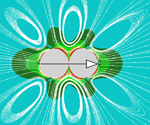
4.2. Pusher–puller dumbbell swims faster than other assemblies
This section further investigates the squirmer dumbbell swimming in a Giesekus fluid. Here, we consider two identical and two different squirmers in assembling the dumbbell for completeness. The main finding in this section is that the pusher–puller (the puller is in front of the pusher) dumbbell swims significantly faster than other dumbbells, as shown in figure 7. For example, its speed is approximately 190% faster than that of the puller–pusher (the pusher is in front of the puller) at Re = 0.01 and Wi = 12. The velocity magnitude around the dumbbells may provide insight into understanding the physics, as shown in figure 8. Comparing figures 8(c) and 8(d), it is seen that the velocity magnitude of the puller–pusher dumbbell is more fore-and-aft symmetric than that of pusher–puller one. For the viscoelastic fluid in the Stokes flow regime, breaking the symmetry of flows around the body is the crucial hydrodynamics for self-propulsion (Pak et al. Reference Pak, Zhu, Brandt and Lauga2012). Hence, the pusher–puller dumbbell uses the hydrodynamic force in self-propulsion better than the puller–pusher one. Meanwhile, the velocity gradient in front of the pusher–puller dumbbell is more significant than that of the puller–pusher one, corresponding to the fact that a more rapid decay yields a faster speed, as mentioned in the above section. For the puller and pusher dumbbells (see figure 8a,b), their velocity magnitudes show a slightly reversed longitudinally (in the swimming direction). It is difficult for this discrepancy to provide an intuitive hydrodynamic mechanism in understanding their different speeds at Wi = 12 (see figure 7). However, the pattern of our results for the squirmer dumbbells (the assembled two identical pullers, pushers or neutral squirmers) is in good agreement with that of an individual squirmer swimming through a Giesekus fluid, especially at  $Wi \ge 6$ (compared with figure 2). Zhu et al. (Reference Zhu, Lauga and Brandt2012) have reported that the region of stretched polymers behind the swimmer becomes thinner and the induced elastic resistance decreases with Wi, thus explaining the slow recovery of the swimming speed with increasing Wi ( $Wi \ge 6$). However, due to the different swimming modes for these three squirmer dumbbells, it is subtle to quantitatively indicate the recovery ratios by analysing the induced fluid fields. We further plot the velocity contours of the puller–pusher (figure 8e) and pusher–puller (figure 8f) on the z-axis. Focusing on the areas at the front and rear of the puller–pusher, we find a greater velocity behind the body than that at its front. As a greater velocity yields a lower pressure, the front and rear pressure difference induces a net pressure opposite to the swimming direction. On the contrary, the pusher–puller induces a net pressure in the swimming direction (see figure 8f, the velocity in front of the pusher–puller is greater than that in its rear). This indicates the possible mechanism for our finding that the pusher–puller swims much faster than the puller–pusher.

Figure 7. Steady swimming speed of squirmer and squirmer dumbbells through a Giesekus fluid with Wi (the unmarked curves (Re) indicate Re = 0.01).

Figure 8. Comparing the velocity magnitudes around the squirmer dumbbells at Re = 0.01 and Wi = 12. (a) Puller–puller (β = 5); (b) pusher–pusher (β = −5); (c) puller–pusher (β = 5, β = −5); (d) pusher–puller (β = −5, β = 5); (e) and ( f), respectively, denote the velocity contours of (c) and (d) on the z-axis. The velocity magnitude is normalized with 2B 1/3.
To further illustrate the possible hydrodynamic mechanism for the faster pusher–puller dumbbell, we plot the schematic shown in figure 9. The swimming of the dumbbells is determined by the flows induced around the bodies. An individual puller (pusher) ‘pulls’ (pushes) the flows to achieve self-propulsion (Li et al. Reference Li, Ostace and Ardekani2016; More & Ardekani Reference More and Ardekani2020; Ouyang et al. Reference Ouyang, Lin, Yu, Lin and Phan-Thien2022), and the assembled dumbbells generate the superimposed flows (see figure 9, the green and blue arrows) induced by the individual squirmers. Since the bigger green and blue arrows in the front or at the rear of the dumbbells are only partly exerted on the sides of the bodies, the smaller green and blue arrows (the dominant role) in the middle of the bodies may help in understanding the driving effects. Note that the smaller arrows in the middle of the bodies indicate the hindrance of the hydrodynamic interactions between the individual squirmers. We find that the pusher–puller induces the superimposed positive driving effect (see figure 9c), in contrast to the puller–pusher, which induces the superimposed negative driving effect (see figure 9d). This results in the fastest pusher–puller and the slowest puller–pusher. Additionally, the middle smaller arrows for puller–puller and pusher–pusher are cancelled (see figure 9a,b), hence their speeds are between the pusher–puller and puller–pusher. However, it is challenging for this schematic to indicate the mechanism of the different speeds between the pusher–pusher and puller–puller.

Figure 9. Schematic to compare the swimming mechanisms between the squirmer dumbbells in an infinite fluid field. (a) Puller–puller dumbbell; (b) pusher–pusher dumbbell; (c) pusher–puller dumbbell; (d) puller–pusher dumbbell. The green and blue swimmers, respectively, denote the puller and the pusher, and the arrows correspond their induced flows. The dashed boundary lines represent the periodic conditions, and the black arrows indicate the swimming direction.
We further focus on the pusher–puller dumbbells to elaborate on essential factors affecting their speed in the viscoelastic fluids. Maintaining the pusher with β = −5, as shown in figure 7, the decrease of the puller (from β = 5 to 3) yields a lower speed, and this pattern applies down to β = 0 (neutral squirmer). This indicates that the front-arranged puller has a positive effect on driving the dumbbell. The speed of the pusher–pullers increases with Re, displaying a similar pattern to that of the individual pusher. Our results also emphasize that, even at a finite but small Reynold number (Re = 5), the fluid inertia rather than the elasticity dominates the pusher–puller (the swimming speed enhances significantly from Re = 0.01 to 5).
4.3. Force contribution analysis
To better understand the possible mechanism for the above results, we examine the force contribution of the squirmers (dumbbells). For a steady swimming squirmer (dumbbell) through a Giesekus fluid, the net force on the body can be decomposed into pressure, viscous and polymeric contributions (force free); in the swimming direction (z-axis), it is  ${F_z} = F_z^{pres} + F_z^{visc} + F_z^{poly} = 0$. The pressure force, the viscous force and the polymeric force have the following forms:
 \begin{gather}F_z^{pres}= - \int_{\partial {P_0}} {{n_z}p\,\textrm{d}S} ,\end{gather}
 \begin{gather}F_z^{visc}= {\eta _s}\int_{\partial {P_0}} {\left[ {2{n_z}\frac{{\partial {u_z}}}{{\partial z}} + {n_x}\left( {\frac{{\partial {u_z}}}{{\partial x}} + \frac{{\partial {u_x}}}{{\partial z}}} \right) + {n_y}\left( {\frac{{\partial {u_z}}}{{\partial y}} + \frac{{\partial {u_y}}}{{\partial z}}} \right)} \right]\textrm{d}S} ,\end{gather}
 \begin{gather}F_z^{poly}= \int_{\partial {P_0}} {[{n_z}{\tau _{zz}} + {n_y}{\tau _{yz}} + {n_x}{\tau _{xz}}]\,\textrm{d}S} ,\end{gather}
where  ${\eta _s}$ denotes the viscosity of the fluid, n is the unit normal outward the surface S of the body. In (4.3), the polymer force can be further decomposed into the normal polymeric force, $F_{zn}^{poly}$, and the polymeric shear force, $F_{zs}^{poly}$
 \begin{gather}F_{zn}^{poly}= \int_{\partial {P_0}} {{n_z}{\tau _{zz}}\,\textrm{d}S} ,\end{gather}
 \begin{gather}F_{zs}^{poly}= \int_{\partial {P_0}} {[{n_y}{\tau _{yz}} + {n_x}{\tau _{xz}}]\,\textrm{d}S} .\end{gather}
 Figure 10 presents the force contributions for a squirmer swimming in a Giesekus fluid, in which the forces are normalized by η 0U 0a. Regarding a neutral squirmer across Re, the viscous force  $F_z^{visc}$ increases monotonically, but the total polymeric force $F_z^{poly}$ almost maintains an unchanged and negative contribution (see figure 10a). This indicates that the increase of the fluid inertia mainly results in the competition between the pressure (not shown) and the viscous force by altering the flows around the body. Meanwhile, $F_z^{visc}$ is dominant in driving (positive contribution) the squirmer, similar to the results of Binagia et al. (Reference Binagia, Phoa, Housiadas and Shaqfeh2020). However, $F_{zn}^{poly}$ makes a more considerable negative contribution than $F_{zs}^{poly}$, in contrast to the results of Binagia et al. (Reference Binagia, Phoa, Housiadas and Shaqfeh2020). This may be because we consider finite fluid inertia here (Re = 5), but the reference adopts swimming that falls into the Stokes flow regime (Re = 0). With fluid inertia, the flows around the body tend to become fore-and-aft asymmetric. This rearranges the distribution and hence the contribution of $F_{zn}^{poly}$. For a pusher (β = −5) across Wi (see figure 10b), we find the total polymeric force $F_z^{poly}$ holds (positive contribution), but $F_z^{visc}$ decreases monotonically (negative contribution) and converges to approximately 31 at Wi = 12. This result is different from the speed of a neutral squirmer (Re = 0) through Giesekus fluids (Binagia et al. Reference Binagia, Phoa, Housiadas and Shaqfeh2020) where the shear polymer force makes a negative contribution. This may be because of the different self-propelling modes and the hydrodynamics (here, we consider a pusher with the finite fluid inertia (Re = 5)). The pattern of $F_z^{visc}$ with Wi also indicates the balance of energy dissipation into the fluids, and the convergent viscous force may indicate a convergent speed, as shown in figure 3. Figure 11 presents the component of the polymer stress τzz distributed around the squirmer. A larger amount of extensional stress in the neutral squirmer's (β = 0) wake is observed at Re = 100 than at Re = 5 (see figure 11a,b). This may be because the fluid inertia contributes to the stretching of the wake. For the viscoelastic fluid, the isotropic polymer stress can be regarded as a ‘pressure’ (Yu et al. Reference Yu, Wang, Lin and Hu2019). We infer that a larger τzz around the rear of the squirmer generates a more significant elasticity-induced force in speeding up the body (along the z-axis). Considering the different self-propelling modes, we find that the pusher induces a more significant τzz at the rear of the body than a neutral squirmer (see figure 11a,c). Moreover, a distinct τzz is also observed at the pusher's sides and front, indicating that the ‘push’ effect results in deforming of the fluids around the body. With the increase of fluid elasticity (increasing Wi up to 12, see figure 11d), τzz around the body becomes weaker. This high elasticity of the fluids resists the deforming flows induced by the slip velocity for driving the body, resulting in a somewhat converged swimming speed with Wi (see figure 3b, the pusher).

Figure 10. Force contribution of a squirmer through a Giesekus fluid. (a) Forces with Re (Wi = 2); (b) forces with Wi (Re = 5).

Figure 11. Component of polymer stress τzz distribution around the squirmer. (a) Wi = 2, β = 0, Re = 5; (b) Wi = 2, β = 0, Re = 100; (c) Wi = 2, β = −5, Re = 5; (d) Wi = 12, β = −5, Re = 5.
The force contribution of the squirmer dumbbell through a Giesekus fluid is presented in figure 12. The viscous force  $F_z^{visc}$ decreases monotonically with Wi, indicating the gradually increasing ratio of the total polymeric force. Swimming in the fluid with low elasticity (e.g. Wi = 1), the viscous force is dominant in driving (positive contribution) the dumbbells. Hence, it can be inferred that the velocity gradient around the dumbbells tends to be fore-and-aft asymmetric based on (4.2). The increase of Wi may induce the strong elastic wake, altering the distribution of the velocity gradient and weakening the viscous force. It can be concluded from figure 12 that the effect of the total polymeric force $F_z^{poly}$ ( $F_{zn}^{poly} + F_{zs}^{poly}$) is generally weaker than the viscous force. This indicates that the inclusion of fluid elasticity is not essential for the different swimming speeds between the pusher–puller and the puller–pusher, and the method of assembly may determine if they can effectively utilize the hydrodynamics for driving or not.

Figure 12. Force contribution of a squirmer dumbbell through a Giesekus fluid with Wi (Re = 0.01). (a) Pusher–puller (|β| = 5); (b) puller–pusher (|β| = 5).
4.4. Energy expenditure and hydrodynamic efficiency
For a squirmer or squirmer dumbbell swimming through the fluids, the rate of work P can be written as
 \begin{equation}P ={-} \int_{\partial {P_0}} {(\boldsymbol{u}\boldsymbol{\cdot }\boldsymbol{\sigma })\boldsymbol{\cdot }\boldsymbol{n}\,\textrm{d}S} ,\end{equation}
where n is the unit normal outward the surface S of the swimmer, and σ denotes the total stress tensor. Figure 13 presents the energy expenditure for the steady swimming of a squirmer and squirmer dumbbell through a Giesekus fluid, in which P is normalized with PN (PN is defined as the power at a Newtonian (Wi = 0) fluid for the squirmer (dumbbell) with the same gait). Swimming in viscoelastic fluids (Wi = 2), as shown in figure 12(a), expends less energy than its Newtonian counterpart. This pattern is similar to that of a neutral squirmer (β = 0) swimming through viscoelastic fluids at Re = 0 (Binagia et al. Reference Binagia, Phoa, Housiadas and Shaqfeh2020). The fluid inertia results in a decrease of energy expenditure, and the neutral squirmer maintains a larger P than that of the pusher or puller. At the finite Re = 5, as shown in figure 12(b), the normalized P decreases monotonically with Wi, in agreement with the pattern of a squirmer swimming at Re = 0 (Binagia et al. Reference Binagia, Phoa, Housiadas and Shaqfeh2020). Meanwhile, it is seen that the energy expenditure is relevant with the steady swimming speeds, in which the faster counterpart squirmer (dumbbell) expends less energy. We further consider the hydrodynamic efficiency η = P*/P, as shown in figure 14, in which P* denotes the power necessary to move the swimmer at its swimming speed U. Note that P* is obtained numerically. For viscoelastic fluids (Wi = 2, see figure 14a), η of the squirmer increases monotonically with Re. This pattern is also reported for the swimming of a squirmer in a Newtonian fluid. However, here we observe the divergent results with Re (in a Newtonian fluid, η of a counterpart squirmer presents only a perceptible difference up to Re = 100 (Chisholm et al. Reference Chisholm, Legendre, Lauga and Khair2016)). Figure 14(b) presents η of an inertial squirmer (dumbbell) swimming through viscoelastic fluids (Re = 5). It is seen that η displays a positive relationship with the swimming speed of the counterpart swimmers, and the increase of Wi results in the increase of η. This result reproduces the conclusion that the elasticity of the fluid contributes to the enhancement of swimming efficiency (Zhu et al. Reference Zhu, Lauga and Brandt2012; Binagia et al. Reference Binagia, Phoa, Housiadas and Shaqfeh2020), and this is regardless of fluid inertia.

Figure 13. Energy expenditure for the steady swimming of a squirmer and squirmer dumbbell through a Giesekus fluid: (a) Wi = 2; (b) Re = 5.

Figure 14. Hydrodynamic efficiency for the steady swimming of a squirmer and squirmer dumbbell through a Giesekus fluid: (a) Wi = 2; (b) Re = 5.
5. Conclusion
We have studied the hydrodynamics of a spherical and a dumbbell-shaped squirmer in a Giesekus fluid. By systematically considering the swimmers’ speed, energy expenditure and hydrodynamic efficiency, we attempt to shed light on how the fluid inertia and elasticity jointly affect their hydrodynamic behaviours. Our results indicate that, for the neutral squirmer, its speed increases monotonically with increasing Reynolds number in a Giesekus fluid, in contrast to holding a constant speed in a Newtonian one. Meanwhile, the speed of the finite inertial squirmer increases monotonically with Wi. This may be due to the different fluid stresses generated in the extensional flow at the rear of the squirmer. Specifically, the increasing Wi results in better convection of the vorticity downstream, subsequently speeding up the puller and pusher.
Regarding the dumbbell squirmer, it is found that the pusher–puller dumbbell swims significantly faster than other dumbbells. For example, its speed can be approximately twice as fast as that of the puller–pusher. This is because the flow field of a pusher–puller dumbbell tends to become more fore-and-aft asymmetric than that of other dumbbells, inducing a significant hydrodynamic self-propulsion force. Moreover, the pusher–puller dumbbell induces flows, which is more beneficial in the positive superposition for driving the body.
Additionally, we find swimming in a viscoelastic fluid expends less energy than its Newtonian counterpart, and the fluid inertia results in a decrease of energy expenditure. The energy expenditure is shown to be relevant at steady swimming speeds, in which the faster counterpart squirmer (dumbbell) expends less energy. The hydrodynamic efficiency η increases monotonically with Re, and also with Wi. This pattern also displays a positive relationship with the swimming speed of the counterpart swimmers.
Funding
The authors would like to thank the Major Program of National Natural Science Foundation of China (Grant Nos. 12132015) and National Natural Science Foundation of China (Grant Nos. 12172327; 11972203).
Declaration of interests
The authors report no conflict of interest.
Data availability
The data that support the findings of this study are available from the corresponding author upon reasonable request.
Appendix A. On the details of solving (2.6)
The set of equations related to  $\boldsymbol{\varLambda }$ have the following forms:
 \begin{equation}\left. {\begin{array}{c@{}} {\dfrac{{\partial {{\tilde{l}}_{ii}}}}{{\partial t}} = {g_{ii}} - \boldsymbol{u}\boldsymbol{\cdot }\boldsymbol{\nabla }{{\tilde{l}}_{ii}},}\\ {\dfrac{{\partial {l_{ij(j > i)}}}}{{\partial t}} = {g_{ij}} - \boldsymbol{u}\boldsymbol{\cdot }\boldsymbol{\nabla }{l_{ij}},} \end{array}} \right\}\end{equation}
where the details of gij read as
 \begin{equation}
\left.
\begin{aligned}
{g_{11}} &=\dfrac{1}{2}\,{\textrm{e}^{( -2{{\tilde{l}}_{11}})}}{c_{11}},\\
{g_{21}} &={\textrm{e}^{( - {{\tilde{l}}_{11}})}}{c_{12}} -\dfrac{{{l_{21}}}}{2}\,{\textrm{e}^{( -2{{\tilde{l}}_{11}})}}{c_{11}},\\
{g_{31}} &={\textrm{e}^{( - {{\tilde{l}}_{11}})}}{c_{13}} -\dfrac{{{l_{31}}}}{2}\,{\textrm{e}^{( -2{{\tilde{l}}_{11}})}}{c_{11}},\\
{g_{22}} &=\dfrac{1}{2}\,{\textrm{e}^{( -2{{\tilde{l}}_{22}})}}{c_{22}} - {l_{21}}\,{e^{( -{{\tilde{l}}_{11}} - 2{{\tilde{l}}_{22}})}}{c_{12}} +\dfrac{1}{2}l_{21}^2\,{e^{( - 2{{\tilde{l}}_{11}} -2{{\tilde{l}}_{22}})}}{c_{11}},\\
{g_{32}} &= {\textrm{e}^{( - {{\tilde{l}}_{22}})}}{c_{23}} -\dfrac{{{l_{32}}}}{2}\,{\textrm{e}^{( -2{{\tilde{l}}_{22}})}}{c_{22}} - {l_{21}}\,{\textrm{e}^{( - {{\tilde{l}}_{11}} - {{\tilde{l}}_{22}})}}{c_{13}} -({l_{22}}{l_{31}} - {l_{21}}{l_{32}})\,{\textrm{e}^{( -{{\tilde{l}}_{11}} - 2{{\tilde{l}}_{22}})}}{c_{12}}\\
&\quad +\dfrac{1}{2}[2{l_{21}}\,{\textrm{e}^{({{\tilde{l}}_{22}})}}{l_{31}}- l_{21}^2{l_{32}}]\,{\textrm{e}^{( - 2{{\tilde{l}}_{11}} -2{{\tilde{l}}_{22}})}}{c_{11}},\\
{g_{33}} &= \dfrac{1}{2}\,{\textrm{e}^{( -2{{\tilde{l}}_{33}})}}{c_{33}} - {l_{32}}\,{\textrm{e}^{( -{{\tilde{l}}_{22}} - 2{{\tilde{l}}_{33}})}}{c_{23}} + \dfrac{{l_{32}^2}}{2}\,{\textrm{e}^{( - 2{{\tilde{l}}_{22}}- 2{{\tilde{l}}_{33}})}}{c_{22}}\\
&\quad -[{\textrm{e}^{({{\tilde{l}}_{22}})}}{l_{31}}- {l_{21}}{l_{32}}]\,{\textrm{e}^{( - {{\tilde{l}}_{11}} -{{\tilde{l}}_{22}} - 2{{\tilde{l}}_{33}})}}{c_{13}}\\
&\quad +{l_{32}}[{\textrm{e}^{({{\tilde{l}}_{22}})}}{l_{31}} -{l_{21}}{l_{32}}]\,{\textrm{e}^{( - {{\tilde{l}}_{11}} - 2{{\tilde{l}}_{22}} - 2{{\tilde{l}}_{33}})}}{c_{12}}\\
&\quad +\dfrac{1}{2}[{\textrm{e}^{(2{{\tilde{l}}_{22}})}}l_{31}^2 -2{l_{21}}\,{\textrm{e}^{({{\tilde{l}}_{22}})}}{l_{31}}{l_{32}} + l_{21}^2l_{32}^2]\,{\textrm{e}^{( - 2{{\tilde{l}}_{11}} -2{{\tilde{l}}_{22}} - 2{{\tilde{l}}_{33}})}}{c_{11}},
\end{aligned}\right\}
\end{equation}
\begin{equation}
\left.
\begin{aligned}
{g_{11}} &=\dfrac{1}{2}\,{\textrm{e}^{( -2{{\tilde{l}}_{11}})}}{c_{11}},\\
{g_{21}} &={\textrm{e}^{( - {{\tilde{l}}_{11}})}}{c_{12}} -\dfrac{{{l_{21}}}}{2}\,{\textrm{e}^{( -2{{\tilde{l}}_{11}})}}{c_{11}},\\
{g_{31}} &={\textrm{e}^{( - {{\tilde{l}}_{11}})}}{c_{13}} -\dfrac{{{l_{31}}}}{2}\,{\textrm{e}^{( -2{{\tilde{l}}_{11}})}}{c_{11}},\\
{g_{22}} &=\dfrac{1}{2}\,{\textrm{e}^{( -2{{\tilde{l}}_{22}})}}{c_{22}} - {l_{21}}\,{e^{( -{{\tilde{l}}_{11}} - 2{{\tilde{l}}_{22}})}}{c_{12}} +\dfrac{1}{2}l_{21}^2\,{e^{( - 2{{\tilde{l}}_{11}} -2{{\tilde{l}}_{22}})}}{c_{11}},\\
{g_{32}} &= {\textrm{e}^{( - {{\tilde{l}}_{22}})}}{c_{23}} -\dfrac{{{l_{32}}}}{2}\,{\textrm{e}^{( -2{{\tilde{l}}_{22}})}}{c_{22}} - {l_{21}}\,{\textrm{e}^{( - {{\tilde{l}}_{11}} - {{\tilde{l}}_{22}})}}{c_{13}} -({l_{22}}{l_{31}} - {l_{21}}{l_{32}})\,{\textrm{e}^{( -{{\tilde{l}}_{11}} - 2{{\tilde{l}}_{22}})}}{c_{12}}\\
&\quad +\dfrac{1}{2}[2{l_{21}}\,{\textrm{e}^{({{\tilde{l}}_{22}})}}{l_{31}}- l_{21}^2{l_{32}}]\,{\textrm{e}^{( - 2{{\tilde{l}}_{11}} -2{{\tilde{l}}_{22}})}}{c_{11}},\\
{g_{33}} &= \dfrac{1}{2}\,{\textrm{e}^{( -2{{\tilde{l}}_{33}})}}{c_{33}} - {l_{32}}\,{\textrm{e}^{( -{{\tilde{l}}_{22}} - 2{{\tilde{l}}_{33}})}}{c_{23}} + \dfrac{{l_{32}^2}}{2}\,{\textrm{e}^{( - 2{{\tilde{l}}_{22}}- 2{{\tilde{l}}_{33}})}}{c_{22}}\\
&\quad -[{\textrm{e}^{({{\tilde{l}}_{22}})}}{l_{31}}- {l_{21}}{l_{32}}]\,{\textrm{e}^{( - {{\tilde{l}}_{11}} -{{\tilde{l}}_{22}} - 2{{\tilde{l}}_{33}})}}{c_{13}}\\
&\quad +{l_{32}}[{\textrm{e}^{({{\tilde{l}}_{22}})}}{l_{31}} -{l_{21}}{l_{32}}]\,{\textrm{e}^{( - {{\tilde{l}}_{11}} - 2{{\tilde{l}}_{22}} - 2{{\tilde{l}}_{33}})}}{c_{12}}\\
&\quad +\dfrac{1}{2}[{\textrm{e}^{(2{{\tilde{l}}_{22}})}}l_{31}^2 -2{l_{21}}\,{\textrm{e}^{({{\tilde{l}}_{22}})}}{l_{31}}{l_{32}} + l_{21}^2l_{32}^2]\,{\textrm{e}^{( - 2{{\tilde{l}}_{11}} -2{{\tilde{l}}_{22}} - 2{{\tilde{l}}_{33}})}}{c_{11}},
\end{aligned}\right\}
\end{equation}
with
 \begin{equation}\left.
\begin{aligned}
{c_{11}} &= 2\left( {{b_{11}}\dfrac{{\partial u}}{{\partial x}} + {b_{12}}\dfrac{{\partial u}}{{\partial y}} +
{b_{13}}\dfrac{{\partial u}}{{\partial z}}} \right)\\ &\quad
- \dfrac{1}{{Wi}}[\alpha (b_{11}^2 + b_{12}^2 + b_{13}^2) + (1 - 2\alpha ){b_{11}} - (1 - \alpha )],\\
{c_{12}} &= \left[ {\left( {{b_{11}}\dfrac{{\partial v}}{{\partial x}} + {b_{12}}\dfrac{{\partial v}}{{\partial y}} +
{b_{13}}\dfrac{{\partial v}}{{\partial z}}} \right) + \left( {{b_{12}}\dfrac{{\partial u}}{{\partial x}} + {b_{22}}\dfrac{{\partial u}}{{\partial y}} +
{b_{23}}\dfrac{{\partial u}}{{\partial z}}} \right)} \right]\\ &\quad - \dfrac{1}{{Wi}}[\alpha
({b_{11}}{b_{12}} + {b_{12}}{b_{22}} + {b_{13}}{b_{23}}) + (1 - 2\alpha ){b_{12}}], \\
{c_{13}} &= \left[ {\left( {{b_{11}}\dfrac{{\partial w}}{{\partial x}} + {b_{12}}\dfrac{{\partial w}}{{\partial
y}} + {b_{13}}\dfrac{{\partial w}}{{\partial z}}} \right) + \left( {{b_{13}}\dfrac{{\partial u}}{{\partial x}} +
{b_{23}}\dfrac{{\partial u}}{{\partial y}} + {b_{33}}\dfrac{{\partial u}}{{\partial z}}} \right)}
\right]\\ &\quad - \dfrac{1}{{Wi}}[\alpha ({b_{11}}{b_{13}} + {b_{12}}{b_{23}} + {b_{13}}{b_{33}}) + (1 - 2\alpha ){b_{13}}],\\
{c_{22}} &= 2\left( {{b_{12}}\dfrac{{\partial v}}{{\partial x}} + {b_{22}}\dfrac{{\partial v}}{{\partial y}} +
{b_{23}}\dfrac{{\partial v}}{{\partial z}}} \right)\\ &\quad - \dfrac{1}{{Wi}}[\alpha (b_{12}^2 + b_{22}^2 +
b_{23}^2) + (1 - 2\alpha ){b_{22}} - (1 - \alpha )],\\
{c_{23}} &= \left[ {\left( {{b_{12}}\dfrac{{\partial w}}{{\partial x}} + {b_{22}}\dfrac{{\partial w}}{{\partial y}} +
{b_{23}}\dfrac{{\partial w}}{{\partial z}}} \right) + \left( {{b_{13}}\dfrac{{\partial v}}{{\partial x}} + {b_{23}}\dfrac{{\partial v}}{{\partial y}} +
{b_{33}}\dfrac{{\partial v}}{{\partial z}}} \right)} \right]\\ &\quad - \dfrac{1}{{Wi}}[\alpha
({b_{12}}{b_{13}} + {b_{22}}{b_{23}} + {b_{23}}{b_{33}}) + (1 - 2\alpha ){b_{23}}], \\
{c_{33}} &= 2\left( {{b_{13}}\dfrac{{\partial w}}{{\partial x}} + {b_{23}}\dfrac{{\partial w}}{{\partial y}} +
{b_{33}}\dfrac{{\partial w}}{{\partial z}}} \right)\\ &\quad - \dfrac{1}{{Wi}}[\alpha (b_{13}^2 + b_{23}^2 +
b_{33}^2) + (1 - 2\alpha ){b_{33}} - (1 - \alpha )]. \end{aligned}
\right\}\end{equation}
\begin{equation}\left.
\begin{aligned}
{c_{11}} &= 2\left( {{b_{11}}\dfrac{{\partial u}}{{\partial x}} + {b_{12}}\dfrac{{\partial u}}{{\partial y}} +
{b_{13}}\dfrac{{\partial u}}{{\partial z}}} \right)\\ &\quad
- \dfrac{1}{{Wi}}[\alpha (b_{11}^2 + b_{12}^2 + b_{13}^2) + (1 - 2\alpha ){b_{11}} - (1 - \alpha )],\\
{c_{12}} &= \left[ {\left( {{b_{11}}\dfrac{{\partial v}}{{\partial x}} + {b_{12}}\dfrac{{\partial v}}{{\partial y}} +
{b_{13}}\dfrac{{\partial v}}{{\partial z}}} \right) + \left( {{b_{12}}\dfrac{{\partial u}}{{\partial x}} + {b_{22}}\dfrac{{\partial u}}{{\partial y}} +
{b_{23}}\dfrac{{\partial u}}{{\partial z}}} \right)} \right]\\ &\quad - \dfrac{1}{{Wi}}[\alpha
({b_{11}}{b_{12}} + {b_{12}}{b_{22}} + {b_{13}}{b_{23}}) + (1 - 2\alpha ){b_{12}}], \\
{c_{13}} &= \left[ {\left( {{b_{11}}\dfrac{{\partial w}}{{\partial x}} + {b_{12}}\dfrac{{\partial w}}{{\partial
y}} + {b_{13}}\dfrac{{\partial w}}{{\partial z}}} \right) + \left( {{b_{13}}\dfrac{{\partial u}}{{\partial x}} +
{b_{23}}\dfrac{{\partial u}}{{\partial y}} + {b_{33}}\dfrac{{\partial u}}{{\partial z}}} \right)}
\right]\\ &\quad - \dfrac{1}{{Wi}}[\alpha ({b_{11}}{b_{13}} + {b_{12}}{b_{23}} + {b_{13}}{b_{33}}) + (1 - 2\alpha ){b_{13}}],\\
{c_{22}} &= 2\left( {{b_{12}}\dfrac{{\partial v}}{{\partial x}} + {b_{22}}\dfrac{{\partial v}}{{\partial y}} +
{b_{23}}\dfrac{{\partial v}}{{\partial z}}} \right)\\ &\quad - \dfrac{1}{{Wi}}[\alpha (b_{12}^2 + b_{22}^2 +
b_{23}^2) + (1 - 2\alpha ){b_{22}} - (1 - \alpha )],\\
{c_{23}} &= \left[ {\left( {{b_{12}}\dfrac{{\partial w}}{{\partial x}} + {b_{22}}\dfrac{{\partial w}}{{\partial y}} +
{b_{23}}\dfrac{{\partial w}}{{\partial z}}} \right) + \left( {{b_{13}}\dfrac{{\partial v}}{{\partial x}} + {b_{23}}\dfrac{{\partial v}}{{\partial y}} +
{b_{33}}\dfrac{{\partial v}}{{\partial z}}} \right)} \right]\\ &\quad - \dfrac{1}{{Wi}}[\alpha
({b_{12}}{b_{13}} + {b_{22}}{b_{23}} + {b_{23}}{b_{33}}) + (1 - 2\alpha ){b_{23}}], \\
{c_{33}} &= 2\left( {{b_{13}}\dfrac{{\partial w}}{{\partial x}} + {b_{23}}\dfrac{{\partial w}}{{\partial y}} +
{b_{33}}\dfrac{{\partial w}}{{\partial z}}} \right)\\ &\quad - \dfrac{1}{{Wi}}[\alpha (b_{13}^2 + b_{23}^2 +
b_{33}^2) + (1 - 2\alpha ){b_{33}} - (1 - \alpha )]. \end{aligned}
\right\}\end{equation}


